HyperML: A Boosting Metric Learning Approach in Hyperbolic Space for Recommender Systems

Conference: The Thirteenth ACM International Conference on Web Search and Data Mining; February 3–7, 2020; Houston, TX, USAThe Thirteenth ACM International Conference on Web Search and Data Mining (WSDM’20), February 3–7, 2020, Houston, TX, USAPrice: 15.00DOI: 10.1145/3336191.3371850ISBN: 978-1-4503-6822-3/20/02CCS: Information systems Recommender systemsCCS: Computing methodologies Neural networks

Lucas Vinh Tran Affiliation: Nanyang Technological University, Institute for Infocomm Research, A*STAR email: trandang001@e.ntu.edu.sg , Yi Tay Note: Now at Google Research. Affiliation: Nanyang Technological University email: ytay017@e.ntu.edu.sg , Shuai Zhang Affiliation: University of New South Wales email: shuai.zhang@student.unsw.edu.au , Gao Cong Affiliation: Nanyang Technological University email: gaocong@ntu.edu.sg and Xiaoli Li Affiliation: Institute for Infocomm Research, A*STAR email: xlli@i2r.a-star.edu.sg

Abstract.

This paper investigates the notion of learning user and item representations in non-Euclidean space. Specifically, we study the connection between metric learning in hyperbolic space and collaborative filtering by exploring Möbius gyrovector spaces where the formalism of the spaces could be utilized to generalize the most common Euclidean vector operations. Overall, this work aims to bridge the gap between Euclidean and hyperbolic geometry in recommender systems through metric learning approach. We propose HyperML (Hyperbolic Metric Learning), a conceptually simple but highly effective model for boosting the performance. Via a series of extensive experiments, we show that our proposed HyperML not only outperforms their Euclidean counterparts, but also achieves state-of-the-art performance on multiple benchmark datasets, demonstrating the effectiveness of personalized recommendation in hyperbolic geometry.

Keywords:

Recommender Systems; Collaborative Filtering; Hyperbolic Neural Networks

1. Introduction

A diverse plethora of machine learning models solves the personalized ranking problem in recommender systems via building matching functions (Rendle et al., 2009; Rendle, 2010; Mnih and Salakhutdinov, 2008; He et al., 2017). Across the literature, a variety of matching functions have been traditionally adopted, such as inner product (Rendle et al., 2009), metric learning (Tay et al., 2018a; Hsieh et al., 2017) and/or neural networks (He et al., 2017; He et al., 2018). Among those approaches, metric learning models (e.g., Collaborative Metric Learning (CML) (Hsieh et al., 2017) and Latent Relational Metric Learning (LRML) (Tay et al., 2018a)) are primarily focused on designing distance functions over objects (i.e., between users and items), demonstrating reasonable empirical success for collaborative ranking with implicit feedback. Nevertheless, those matching functions only covered the scope of Euclidean space.

For the first time, our work explores the notion of learning user-item representations in terms of metric learning in hyperbolic space, in which hyperbolic representation learning has recently demonstrated great potential across a diverse range of applications such as learning entity hierarchies (Nickel and Kiela, 2017) and/or natural language processing (Tay et al., 2018b; Dhingra et al., 2018). Due to the exponentially expansion property of hyperbolic space, we discovered that metric learning with the pull-push mechanism in hyperbolic space could boost the performance significantly: moving a point to a certain distance will require a much smaller force in hyperbolic space than in Euclidean space. To this end, in order to perform metric learning in hyperbolic space, we employ Möbius gyrovector spaces to generally formalize most common Euclidean operations such as addition, multiplication, exponential map and logarithmic map (Ganea et al., 2018b; Ungar, 2009).

Moreover, the ultimate goal when embedding a space into another is to preserve distances and more complex relationships. Thus, our work also introduces the definition of distortion to maintain good representations in hyperbolic space both locally and globally, while controlling the performance through the multi-task learning framework. This reinforces the key idea of modeling user-item pairs in hyperbolic space, while maintaining the simplicity and effectiveness of the metric learning paradigm.

We show that a conceptually simple hyperbolic adaptation in terms of metric learning is capable of not only achieving very competitive results, but also outperforming recent advanced Euclidean metric learning models on multiple personalized ranking benchmarks.

Our Contributions

The key contributions of our work are summarized as follows:

•

We investigate the notion of training recommender systems in hyperbolic space as opposed to Euclidean space by exploring Möbius gyrovector spaces with the Riemannian geometry of the Poincaré model. To the best of our knowledge, this is the first work that explores the use of hyperbolic space for metric learning in the recommender systems domain.
•

We devise a new method HyperML (Hyperbolic Metric Learning), a strong competitive metric learning model for one-class collaborative filtering (i.e., personalized ranking). Unlike previous metric learning models, we incorporate a penalty term called distortion to control and balance between accuracy and preservation of distances.
•

We conduct a series of extensive experiments delving into the inner workings of our proposed HyperML on ten public benchmark datasets. Our model demonstrates the effectiveness of hyperbolic geometry, outperforming not only its Euclidean counterparts but also a suite of competitive baselines. Notably, HyperML outperforms the state-of-the-art CML and LRML models, which are also metric learning models in Euclidean space across all benchmarks. We achieve a boosting performance gain over competitors, pulling ahead by up to $32.32\%$ performance in terms of standard ranking metrics.

2. Hyperbolic Metric Learning

This section provides the overall background and outlines the formulation of our proposed model. The key motivation behind our proposed model is to embed the two user-item pairs into hyperbolic space, creating the gradients of pulling the distance between the positive user-item pair close and pushing the negative user-item pair away.

Figure 1 depicts our overall proposed HyperML model. The figures illustrate our two approaches: 1) optimizing the embeddings within the unit ball and 2) transferring the points to the tangent space via the exponential and logarithmic maps for optimization. In the experiments, we also compare the mentioned variants of HyperML where both approaches achieve competitive results compared to Euclidean metric learning models.

2.1. Hyperbolic Geometry & Poincaré Embeddings

The hyperbolic space $\mathbb{D}$ is uniquely defined as a complete and simply connected Riemannian manifold with constant negative curvature (Krioukov et al., 2010). In fact, there are three types of the Riemannian manifolds of constant curvature, which are Euclidean geometry (constant vanishing sectional curvature), spherical geometry (constant positive sectional curvature) and hyperbolic geometry (constant negative sectional curvature). In this paper, we focus on Euclidean space and hyperbolic space due to the key difference in their space expansion. Indeed, hyperbolic spaces expand faster (exponentially) than Euclidean spaces (polynomially). Specifically, for instance, in the two-dimensional hyperbolic space $\mathbb{D}^{2}_{\epsilon}$ of constant curvature $K=-\epsilon^{2}<0$ , $\epsilon>0$ with the hyperbolic radius of $r$ , we have:

(1)

\vskip-4.30554ptL(r)=2\pi\sinh(\epsilon r),

(2)

A(r)=2\pi(\cosh(\epsilon r)-1),

in which $L(r)$ is the length of the circle and $A(r)$ is the area of the disk. Hence, both equations illustrate the exponentially expansion of the hyperbolic space $\mathbb{H}^{2}_{\epsilon}$ with respect to the radius $r$ .

Although hyperbolic space cannot be isometrically embedded into Euclidean space, there exists multiple models of hyperbolic geometry that can be formulated as a subset of Euclidean space and are very insightful to work with, depending on different tasks. In this work, we prefer the Poincaré ball model due to its conformality (i.e., angles are preserved between hyperbolic and Euclidean space) and convenient parameterization (Nickel and Kiela, 2017).

The Poincaré ball model is the Riemannian manifold $\mathcal{P}^{n}=(\mathbb{D}^{n},g_{p})$ , in which $\mathbb{D}^{n}=\{\textbf{x}\in\mathbb{R}^{n}:\|\textbf{x}\|<1\}$ is the open $n$ -dimensional unit ball that is equipped with the metric:

(3)

\vskip-4.30554ptg_{p}(\textbf{x})=\Bigg(\frac{2}{1-\|\textbf{x}\|^{2}}\Bigg)^{2}g_{e},

where $\textbf{x}\in\mathbb{D}^{n}$ ; $\|\cdot\|$ denotes the Euclidean norm; and $g_{e}$ is the Euclidean metric tensor with components $\textbf{I}_{n}$ of $\mathbb{R}^{n}$ .

The induced distance between two points on $\mathbb{D}^{n}$ is given by:

(4)

d_{\mathbb{D}}(\textbf{x},\textbf{y})=\cosh^{-1}\Bigg(1+2\frac{\|\textbf{x}-\textbf{y}\|^{2}}{(1-\|\textbf{x}\|^{2})(1-\|\textbf{y}\|^{2})}\Bigg).

In fact, if we adopt the hyperbolic distance function as a matching function to model the relationships between users and items, the hyperbolic distance $d_{\mathbb{D}}(\textbf{u},\textbf{v})$ between user $u$ and item $v$ could be calculated based on Eqn. (4).

On a side note, let $\textbf{v}_{j}$ and $\textbf{v}_{k}$ represent the items user $i$ liked and did not like with $d_{\mathbb{D}}(\textbf{u}_{i},\textbf{v}_{j})$ and $d_{\mathbb{D}}(\textbf{u}_{i},\textbf{v}_{k})$ are their distances to the user $i$ on hyperbolic space, respectively. Our goal is to pull $\textbf{v}_{j}$ close to $\textbf{u}_{i}$ while pushing $\textbf{v}_{k}$ away from $\textbf{u}_{i}$ . If we consider the triplet as a tree with two children $\textbf{v}_{j}$ , $\textbf{v}_{k}$ of parent $\textbf{u}_{i}$ and place $\textbf{u}_{i}$ relatively close to the origin, the graph distance of $\textbf{v}_{j}$ and $\textbf{v}_{k}$ is obviously calculated as $d(\textbf{v}_{j},\textbf{v}_{k})=d(\textbf{u}_{i},\textbf{v}_{j})+d(\textbf{u}_{i},\textbf{v}_{k})$ , or we will obtain the ratio $\frac{d(\textbf{v}_{j},\textbf{v}_{k})}{d(\textbf{u}_{i},\textbf{v}_{j})+d(\textbf{u}_{i},\textbf{v}_{k})}=1$ . If we embed the triplet in Euclidean space, the ratio $\frac{d_{\mathbb{E}}(\textbf{v}_{j},\textbf{v}_{k})}{d_{\mathbb{E}}(\textbf{u}_{i},\textbf{v}_{j})+d_{\mathbb{E}}(\textbf{u}_{i},\textbf{v}_{k})}$ is constant, which seems not to capture the mentioned graph-like structure. However, in hyperbolic space, the ratio $\frac{d_{\mathbb{D}}(\textbf{v}_{j},\textbf{v}_{k})}{d_{\mathbb{D}}(\textbf{u}_{i},\textbf{v}_{j})+d_{\mathbb{D}}(\textbf{u}_{i},\textbf{v}_{k})}$ approaches 1 as the edges are long enough, which makes the distances nearly preserved (Sala et al., 2018).

Thus, it is worth mentioning our key idea is that for a given triplet, we aim to embed the root (the user) arbitrarily close to the origin and space the children (positive and negative items) around a sphere centered at the parent. Notably, the distances between points grows exponentially as the norm of the vectors approaches 1. Geometrically, if we place the root node of a tree at the origin of $\mathbb{D}^{n}$ , the children nodes spread out exponentially with their distances to the root towards the boundary of the ball due to the above mentioned property.

2.2. Gyrovector spaces

In this section, we make use of Möbius gyrovector spaces operations (Ganea et al., 2018b) to generally design the distance of user-item pairs for further extension.

Specifically, for $c\geq 0$ , we denote $\mathbb{D}_{c}^{n}=\{x\in\mathbb{R}^{n}:c\|x\|^{2}<1\}$ , which is considered as the open ball of radius $\frac{1}{\sqrt{c}}$ . Note that if $c=0$ , we get $\mathbb{D}_{c}^{n}=\mathbb{R}^{n}$ ; and if $c=1$ , we retrieve the usual unit ball as $\mathbb{D}_{c}^{n}=\mathbb{D}^{n}$ .

Some widely used Möbius operations of gyrovector spaces are introduced as follows:

Möbius addition:

The Möbius addition of $x$ and $y$ in $\mathbb{D}_{c}^{n}$ is defined:

(5)

x\oplus_{c}y=\frac{(1+2c\langle x,y\rangle+c\|y\|^{2})x+(1-c\|x\|^{2})y}{1+2c\langle x,y\rangle+c\|x\|^{2}\|y\|^{2}}.

Möbius scalar multiplication:

For $c>0$ , the Möbius scalar multiplication of $x\in\mathbb{D}_{c}^{n}\setminus\{\textbf{0}\}$ with $r\in\mathbb{R}$ is defined:

(6)

r\otimes_{c}x=\frac{1}{\sqrt{c}}\tanh(r\tanh^{-1}(\sqrt{c}\|x\|))\frac{x}{\|x\|},

and $r\otimes_{c}\textbf{0}=\textbf{0}$ . Note that when $c\rightarrow 0$ , we recover the Euclidean addition and scalar multiplication. The Möbius subtraction can also be obtained as $x\ominus_{c}y=x\oplus_{c}(-y)$ .

Möbius exponential and logarithmic maps:

For any $x\in\mathbb{D}_{c}^{n}$ , the Möbius exponential map and logarithmic map, given $v\neq\textbf{0}$ and $y\neq x$ , are defined:

(7)

\exp_{x}^{c}(v)=x\oplus_{c}\Big(\tanh\Big(\sqrt{c}\frac{\lambda_{x}^{c}\|v\|}{2}\Big)\frac{v}{\sqrt{c}\|v\|}\Big),

(8)

\log_{x}^{c}(y)=\frac{2}{\lambda_{x}^{c}\sqrt{c}}\tanh^{-1}(\sqrt{c}\|(-x)\oplus_{c}y\|)\frac{(-x)\oplus_{c}y}{\|(-x)\oplus_{c}y\|},

where $\lambda_{x}^{c}=\frac{2}{1-c\|x\|^{2}}$ is the conformal factor of $(\mathbb{D}_{c}^{n},g^{c})$ in which $g^{c}$ is the generalized hyperbolic metric tensor. We also recover the Euclidean exponential map and logarithmic map as $c\rightarrow 0$ . Readers can refer to (Ganea et al., 2018b; Ungar, 2009) for the detailed introduction to Gyrovector spaces.

We then obtain the generalized distance in Gyrovector spaces:

(9)

d_{c}(x,y)=\frac{2}{\sqrt{c}}\tanh^{-1}(\sqrt{c}\|(-x)\oplus_{c}y\|).

When $c\rightarrow 0$ , we recover the Euclidean distance since we have $\lim_{c\to 0}d_{c}(x,y)=2\|x-y\|$ . When $c=1$ , we retrieve the Eqn. (4). In other words, hyperbolic space resembles Euclidean as it gets closer to the origin, which motivates us to design our loss function in the multi-task learning framework.

2.3. Model Formulation

Our proposed model takes a user (denoted as $\textbf{u}_{i}$ ), a positive (observed) item (denoted as $\textbf{v}_{j}$ ) and a negative (unobserved) item (denoted as $\textbf{v}_{k}$ ) as an input. Each user and item is represented as a one-hot vector which map onto a dense low-dimensional vector by indexing onto an user/item embedding matrix. We learn these vectors with the generalized distance:

(10)

d_{c}(\textbf{u},\textbf{v})=\frac{2}{\sqrt{c}}\tanh^{-1}(\sqrt{c}\|(-\textbf{u})\oplus_{c}\textbf{v}\|),

in which an item $j$ that user $i$ liked (positive) is expected to be closer to the user than the ones he did not like (negative).

In fact, we would like to learn the user-item joint metric to encode the observed positive feedback. Specifically, the learned metric pulls the positive pairs closer and pushes the other pairs further apart.

Notably, this process will also cluster the users who like the same items together, and the items that are liked by the same users together, due to the triangle inequalities. Similar to (Hsieh et al., 2017), for a given user, the nearest neighborhood items are: 1) the items liked by this user previously, and 2) the items liked by other users with similar interests to this user. In other words, we are also able to indirectly observe the relationships between user-user pairs and item-item pairs through the pull-push mechanism of metric learning.

Figure 1. Illustration of our proposed HyperML. The left figure with the greenish ball represents the hyperbolic unit ball and the pale blue parallelogram illustrates its tangent space; red and vermeil circles represent user embeddings; green and purple circles represent item embeddings. The right figure illustrates an example of a triplet embedding of user (red circle), positive item (green circle) and negative item (orange circle), in which it demonstrates a small tree of one root and two children which is embedded into hyperbolic space with the exponentially expansion property (Best viewed in color).

Pull-and-Push Optimization.

To formulate such constraint, we define our pull-and-push loss function as:

(11)

\mathcal{L}_{P}=\sum_{(i,j)\in\mathbb{S}}\sum_{(i,k)\notin\mathbb{S}}[m+d_{\mathbb{D}}^{2}(i,j)-d_{\mathbb{D}}^{2}(i,k)]_{+},

where $j$ is an item user $i$ liked and $k$ is the one he did not like; $\mathbb{S}$ contains all the observed implicit feedback, i.e. positive item-user pairs; $[z]_{+}=\max(0,z)$ is the standard hinge loss; and $m>0$ is the safety margin size. Notably, our loss function does not adopt the ranking loss weight compared to (Hsieh et al., 2017).

Distortion Optimization.

The ultimate goal when embedding a space into another is to preserve distances while maintaining complex structures/relationships (Sala et al., 2018). Thus, it becomes a challenge when embedding user-item pairs to hyperbolic space with the needs of preserving good structure quality for metric learning. To this end, we consider the two factors of good representations namely local and global factor. Locally, the children items must be spread out on the sphere around the parent user as described, with pull and push forces created by the gradients. Globally, the learned triplets should be separated reasonably from each other. While pull-and-push optimization satisfies the local requirement, we define the distortion optimization function to meet the global requirement as:

(12)

\mathcal{L}_{D}=\sum_{(i,j)\in\mathbb{S}}\Big[\frac{|d_{\mathbb{D}}(f(i),f(j))-d_{\mathbb{E}}(i,j)|}{d_{\mathbb{E}}(i,j)}\Big]_{+}\\ +\sum_{(i,k)\notin\mathbb{S}}\Big[\frac{|d_{\mathbb{D}}(f(i),f(k))-d_{\mathbb{E}}(i,k)|}{d_{\mathbb{E}}(i,k)}\Big]_{+},

where $|\cdot|$ defines the absolute value; and $f(\cdot)$ is a mapping function $f:\mathbb{E}\rightarrow\mathbb{D}$ from Euclidean space $\mathbb{E}$ to hyperbolic space $\mathbb{D}$ . In this paper, we take $f(\cdot)$ as an identity function.

We aim to preserve the distances by minimizing $\mathcal{L}_{D}$ for the global factor. Ideally, the lower the distortion, the better the preservation.

Multi-Task Learning.

We then integrate the pull-and-push part (i.e., $\mathcal{L}_{P}$ ) and the distortion part (i.e., $\mathcal{L}_{D}$ ) into an end-to-end fashion through a multi-task learning framework. The objective function is defined as:

(13)

\min_{\Theta}\mathcal{L}=\mathcal{L}_{P}+\gamma\mathcal{L}_{D},

where $\Theta$ is the total parameter space, including all embeddings and variables of the networks; and $\gamma$ is the multi-task learning weight.

There is an unavoidable trade-off between the precision (learned from the pull-push mechanism) and the distortion as similar to (Sala et al., 2018). Thus, jointly training $\mathcal{L}_{P}$ and $\mathcal{L}_{D}$ can help to boost the model performance while providing good representations. Indeed, we examine the performance of HyperML with and without the distortion by varying different multi-task learning weight $\gamma$ in our experiment in Section 3.

Gradient Conversion.

The parameters of our model are learned by projected Riemannian stochastic gradient descent (RSGD) (Nickel and Kiela, 2017) with the form:

(14)

\boldsymbol{\theta}_{t+1}=\mathfrak{R}_{\theta_{t}}(-\eta_{t}\nabla_{R}\mathcal{L}(\boldsymbol{\theta}_{t})),

where $\mathfrak{R}_{\theta_{t}}$ denotes a retraction onto $\mathbb{D}$ at $\boldsymbol{\theta}$ and $\eta_{t}$ is the learning rate at time $t$ .

The Riemannian gradient $\nabla_{R}$ is then calculated from the Euclidean gradient by rescaling $\nabla_{E}$ with the inverse of the Poincaré ball metric tensor as $\nabla_{R}=\frac{(1-\|\boldsymbol{\theta}_{t}\|^{2})^{2}}{4}\nabla_{E}$ , in which this scaling factor depends on the Euclidean distance of the point at time $t$ from the origin (Nickel and Kiela, 2017; Tay et al., 2018b). Notably, one could also exploit full RSGD for optimization to perform the updates instead of using first-order approximation to the exponential map (Bonnabel, 2013; Ganea et al., 2018a; Wilson and Leimeister, 2018; Bécigneul and Ganea, 2019).

3. Experiments

3.1. Experimental Setup

Datasets.

Dataset	Interactions	# Users	# Items	% Density
Movie20M	16M	53K	27K	1.15
Movie1M	1M	6K	4K	4.52
Goodbooks	6M	53K	10K	1.14
Yelp	1M	22K	18K	0.26
Meetup	248K	47K	17K	0.03
Clothing	358K	39K	23K	0.04
Sports & Outdoors	368K	36K	18K	0.06
Cell Phones	250K	28K	10K	0.09
Toys & Games	206K	19K	12K	0.09
Automotive	26K	3K	2K	0.49

Table 1. Statistics of all datasets used in our experimental evaluation

Refer to caption — Figure 2. Two-dimensional hyperbolic embedding of ten benchmark datasets in the Poincaré disk using t-SNE. The images illustrate the embedding of user and item pairs after the convergence (Best viewed in color).

To evaluate our experiments, we use a wide spectrum of datasets with diverse domains and densities. The statistics of the datasets are reported in Table 1.

•

MovieLens: A widely adopted benchmark dataset in the application domain of recommending movies to users provided by GroupLens research¹¹ 1 https://grouplens.org/datasets/movielens/. We use two configurations, namely MovieLens20M and MovieLens1M. Similar to (Tay et al., 2018a), the MovieLens20M datasets are filtered with 100-core setting.
•

Goodbooks: A large book recommendation dataset contains six million ratings for ten thousand most popular (with most ratings) books.²² 2 https://github.com/zygmuntz/goodbooks-10k
•

Yelp: A crowd-sourced platform for local businesses such as restaurants, bars, etc. We use the dataset from the 2018 edition of the Yelp Dataset Challenge.³³ 3 https://www.yelp.com/dataset/challenge
•

Meetup: An event-based social network dataset. We use the dataset includes event-user pairs from NYC that was provided by (Pham et al., 2016).
•

Amazon Reviews: The amazon review datasets that was introduced in (He and McAuley, 2016a). The subsets⁴⁴ 4 Datasets are obtained from http://jmcauley.ucsd.edu/data/amazon/ using the 5-core setting with the domain names truncated in the interest of space. are selected based on promoting diversity based on dataset size and domain.

MovieLens20M

MovieLens1M

Goodbooks

Yelp

Meetup

nDCG@10

HR@10

nDCG@10

HR@10

nDCG@10

HR@10

nDCG@10

HR@10

nDCG@10

HR@10

MF-BPR

63.462

82.206

55.173

74.057

49.559

71.033

56.443

77.926

48.359

62.468

MLP

62.500

84.380

54.851

73.812

48.597

70.226

52.777

75.784

43.310

55.616

NCF

59.485

81.859

55.503

74.127

50.823

72.014

53.078

72.757

52.334

62.210

CML

62.664

85.571

55.737

74.528

49.010

72.556

54.996

77.122

51.453

60.589

LRML

63.775

81.327

54.057

73.358

50.392

71.424

54.719

76.764

50.208

61.347

HyperML

64.042

87.363

56.197

75.629

51.088

74.152

59.543

81.392

54.633

67.304

Improvement

+0.42%

+2.09%

+0.83%

+1.48%

+0.52%

+2.20%

+5.49%

+4.45%

+4.39%

+7.74%

Clothing

Sports

Cell phones

Games

Automotive

nDCG@10

HR@10

nDCG@10

HR@10

nDCG@10

HR@10

nDCG@10

HR@10

nDCG@10

HR@10

MF-BPR

13.189

20.509

26.130

38.553

26.483

37.434

22.156

34.877

20.433

31.707

MLP

13.947

22.726

24.431

37.015

25.732

37.677

21.074

32.251

16.789

27.685

NCF

16.809

26.470

20.268

30.232

22.496

32.697

20.959

30.871

17.340

28.441

CML

16.623

26.371

19.211

30.197

19.320

29.746

21.579

32.524

17.556

27.985

LRML

16.643

26.421

22.938

33.667

20.177

30.999

20.747

31.695

16.492

26.124

HyperML

17.150

27.899

34.576

48.262

29.325

42.921

23.164

35.995

24.736

37.324

Improvement

+2.03%

+5.40%

+32.32%

+25.18%

+10.73%

+13.92%

+4.55%

+3.21%

+21.06%

+17.72%

Table 2. Experimental results (nDCG@10 and HR@10) on ten public benchmark datasets. Best result is in bold face and second best is underlined. Our proposed HyperML achieves very competitive results, outperforming strong recent advanced metric learning baselines such as CML and LRML.

Evaluation Protocol and Metrics.

We experiment on the one-class collaborative filtering setup. We adopt nDCG@10 (normalized discounted cumulative gain) and HR@10 (Hit Ratio) evaluation metrics, which are well-established ranking metrics for recommendation task. Following (He et al., 2017; Tay et al., 2018a), we randomly select 100 negative samples which the user have not interacted with and rank the ground truth amongst these negative samples. For all datasets, the last item the user has interacted with is withheld as the test set while the penultimate serves as the validation set. During training, we report the test scores of the model based on the best validation scores. All models are evaluated on the validation set at every 50 epochs.

Compared Baselines

In our experiments, we compare with five well-established and competitive baselines which in turn employ different matching functions: inner product (MF-BPR), neural networks (MLP, NCF) and metric learning (CML, LRML).

•

Matrix Factorization with Bayesian Personalized Ranking (MF-BPR) (Rendle et al., 2009) is the standard and strong collaborative filtering (CF) baseline for recommender systems. It models the user-item representation using the inner product and explores the triplet objective to rank items.
•

Multi-layered Perceptron (MLP) is a feedforward neural network that applies multiple layers of nonlinearities to capture the relationship between users and items. We select the best number of MLP layers from $\{3,4,5\}$ .
•

Neural Collaborative Filtering (NCF) (He et al., 2017) is a neural network based method for collaborative filtering which models nonlinear user-item interaction. The key idea of NCF is to fuse the last hidden representation of MF and MLP into a joint model. Following (He et al., 2017), we use a three layered MLP with a pyramid structure.
•

Collaborative Metric Learning (CML) (Hsieh et al., 2017) is a strong metric learning baseline that learns user-item similarity using the Euclidean distance. CML can be considered a key ablative baseline in our experiments, signifying the difference between Hyperbolic and Euclidean metric spaces.
•

Latent Relational Metric Learning (LRML) (Tay et al., 2018a) is also a strong metric learning baseline that learns adaptive relation vectors between user and item interactions to find a single optimal translation vector between each user-item pair.

Implementation Details

We implement all models in Tensorflow. All models are trained with the Adam (Kingma and Ba, 2015) or AdaGrad (Duchi et al., 2011) optimizer with learning rates from $\{0.01,0.001,0.0001,0.00001\}$ . The embedding size $d$ of all models is tuned amongst $\{32,64,128\}$ and the batch size $B$ is tuned amongst $\{128,256,512\}$ . The multi-task learning weight $\gamma$ is empirically chosen from $\{0,0.1,0.25,0.5,0.75,\\ 1.0\}$ . For models that optimize the hinge loss, the margin $\lambda$ is selected from $\{0.1,0.2,0.5\}$ . For NCF, we use a pre-trained model as reported in (He et al., 2017) to achieve its best performance. All the embeddings and parameters are randomly initialized using the random uniform initializer $\mathcal{U}(-\alpha,\alpha)$ . For non-metric learning baselines, we set $\alpha=0.01$ . For metric learning models, we empirically set $\alpha=(\frac{3\beta^{2}}{2d})^{\frac{1}{3}}$ , in which we choose $\beta=0.01$ . The reason is that we would like all the embeddings of the metric learning models to be initialized arbitrarily close to the origin of the balls⁵⁵ 5 The balls are referred as hyperbolic ball for HyperML model and Euclidean ball for CML and LRML model. for a fair comparison. For most datasets and baselines, we empirically set the embedding size of $64$ and the batch size is $512$ . We also empirically set the dropout rate $\rho=0.5$ to prevent overfitting. For each dataset, the optimal parameters are established by repeating each experiment for $N$ runs and assessing the average results. We have used $N=5$ for our experiment.

3.2. Experimental Results

This section presents our experimental results on all datasets. For all obtained results, the best result is in boldface whereas the second best is underlined. As reported in Table 2, our proposed model consistently outperforms all the baselines on both HR@10 and nDCG@10 metrics across all benchmark datasets.

Pertaining to the baselines, we observe that there is no obvious winner among the baseline solutions. In addition, we also observe that the performance of MF-BPR and CML is extremely competitive, i.e. both MF-BPR and CML consistently achieve good results across the datasets. Notably, the performance of MF-BPR is much better than CML on datasets with less number of interactions. For datasets with larger size (i.e., MovieLens20M, MovieLens1M and Goodbooks), the performance of metric learning models perform better in which the gain of CML and LRML on the non-metric learning baselines across large datasets is approximately +0.39% and +0.91% respectively in terms of nDCG. One possible reason is that for small datasets with low interactions (e.g., Automotive with 26K interactions of $0.49\%$ density), a simple model such as MF-BPR should be considered as a priority choice. In addition, the performance of a careful pre-trained NCF also often achieves competitive results with large datasets but not small ones in most cases. The explanation is because using the dual embedding spaces (since NCF combines MLP and MF) could possibly lead to overfitting if the dataset is not large enough (Tay et al., 2018a).

Remarkably, our proposed model HyperML demonstrates highly competitive results and consistently outperforms the best baseline method. The percentage improvements in terms of nDCG on ten datasets (in the same order as reported in Table 2) are +0.42%, +0.83%, +0.52%, +5.49%, +4.39%, +2.03%, +32.32%, +10.71%, +4.55% and +21.06% respectively. We also observe similar high performance gains on the hit ratio (HR@10). Note that the hyperbolic spaces expand faster, i.e. exponentially, than Euclidean spaces, in which the forces are generated by the rescaled gradients, pulling and pushing the points with more reasonable distances compared to Euclidean. Therefore, it enables us to achieve very competitive results of our proposed HyperML in the hyperbolic space over other strong Euclidean baselines. Our experimental evidence shows the remarkable recommendation results of our proposed HyperML model on the variety of datasets and the advantage of hyperbolic space over Euclidean space in boosting the performance in metric learning framework.

3.3. Model Convergence Analysis

This section investigates the model convergence analysis of our proposed model to understand the behavior of the embeddings in hyperbolic space.

Hyperbolic Convergence

Figure 2 visualizes the two-dimensional hyperbolic embedding using t-SNE on the test set of ten benchmark datasets after the convergence. We observe that item embeddings form a sphere over the user embeddings. Moreover, since we conduct the analysis on the test set, the visualization of the user/item embeddings in Figure 2 demonstrates the ability of HyperML to self-organize and automatically spread out the item embeddings on the sphere around user embeddings, as mentioned in (Tay et al., 2018a; Sala et al., 2018; Tifrea et al., 2019). Moreover, the clustering characteristic of observing the user-user and item-item relationships discussed in Section 2 is also captured in Figure 2. It could be seen especially clearly for the MovieLens and Yelp dataset.

Convergence Comparison

Figure 3 illustrates the comparison between two-dimensional Poincaré embedding (HyperML) and Euclidean embedding (CML, LRML) on the Yelp and Amazon dataset. For the Euclidean embedding, we clip the norm (i.e., the norm of the embeddings is constrained to 1) and initialize all the embeddings very close to the origin, for an analogous comparison.

At first glance, we notice the difference between the three types of embedding by observing the distribution of user and item embeddings in the spaces after the convergence. While HyperML and CML have the item embeddings gradually assemble to a sphere structure surround user embeddings, the item embeddings of LRML have the opposite movement. The reason is because the motivation behind both CML and HyperML is to create the learned metric through the pull-push mechanism, whereas the motivation of LRML is to additionally learn the translation vector, which establishes the main cause of different visualizations.

It is worth mentioning that since we initialize all the embeddings very close to the origin, we observe the difference between hyperbolic and Euclidean space that leads to the difference in the convergence of HyperML and CML. While both models form a sphere shape over the user embeddings equally, we observe that the user embeddings of HyperML tend to be located closer to the origin than CML while we get similar spread out observation of items. The explanation is that even with similar forces created by the gradients in the same direction, the different expansion property of the two spaces produces the distances between the triplets more separable, which leads to the boosting performance of the proposed model.

3.4. Comparison of Hyperbolic Variants

In this section, we study the variants of our proposed model: HyperML and HyperTS (applied optimization after mapping the user and item embeddings to the tangent space at 0 using the $\log_{\textbf{0}}$ map). Notably, HyperTS is viable because the tangent space at the origin of the Poincaré ball resembles Euclidean space. Table 3 represents the performance of the variants on the datasets in terms of nDCG@10 and HR@10. In general, we observe both HyperML and HyperTS achieve highly competitive results, boosting the performance over Euclidean metric learning models across Meetup, Clothing, Sports, and Cell phones datasets.

Meetup

Clothing

nDCG@10

HR@10

nDCG@10

HR@10

HyperML

54.633

67.304

17.150

27.899

HyperTS

54.612

67.277

17.190

27.959

Sports

Cell phones

nDCG@10

HR@10

nDCG@10

HR@10

HyperML

34.576

48.262

29.325

42.921

HyperTS

31.896

45.272

29.933

43.532

Table 3. Performance comparison between HyperML and HyperTS.

3.5. Effect of Scaling Variable

In this section, we study the effect of the variable $c$ on our proposed HyperML and the CML baseline model. Table 4 represents the performance of HyperML regarding the different value of the scaling variable $c$ comparing to CML in terms of nDCG@10. We observe that HyperML achieves best performance when $c=0.5$ on Goodbooks dataset, but $c=2.0$ on Games dataset. For other values of $c$ , we notice the oscillated performance of HyperML.

As introduced, for $c>0$ , our ball shrinks to the radius of $\frac{1}{\sqrt{c}}$ . Without loss of generality, the case of $c>0$ can be reduced to $c=1$ (the usual unit ball). However, we observe that different scaling variable $c$ would effect the performance differently in practice, which should be set carefully for each dataset. In fact, with $c$ carries values from 0.5 to 8.0, the percentage gain/loss of HyperML over CML varies from $+4.87\%/-17.39\%$ to $+14.17\%/-12.71\%$ on Goodbooks and Games dataset, respectively.

Scaling	Goodbooks			Games
Variable $c$	HyperML	CML	$\Delta\textit{(\%)}$	HyperML	CML	$\Delta\textit{(\%)}$
$c=0.5$	51.396	49.010	$+4.87\%$	37.134	32.524	$+14.17\%$
$c=1.0$	51.088	49.010	$+4.24\%$	35.995	32.524	$+10.67\%$
$c=2.0$	49.631	49.010	$+1.27\%$	38.578	32.524	$+18.61\%$
$c=4.0$	46.017	49.010	$-6.11\%$	35.466	32.524	$+9.05\%$
$c=8.0$	40.488	49.010	$-17.39\%$	28.390	32.524	$-12.71\%$

Table 4. Effects of the scaling variable

c

on Goodbooks and Games datasets in terms of nDCG@10.

3.6. Accuracy Trade-off with Different Multi-task Learning Weight

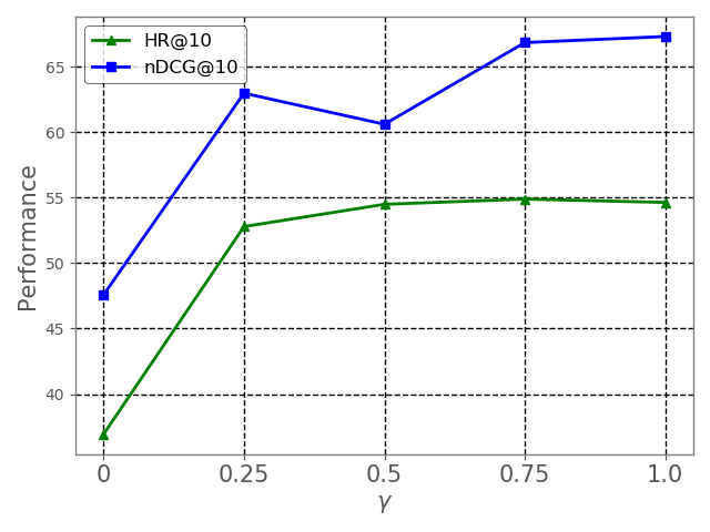
In this section, we study the effect of different multi-task learning weight $\gamma$ on our proposed HyperML model on Meetup and Automotive dataset. Figure 4 represents the performance of HyperML when changing the value of the multi-task learning weight $\gamma$ in terms of HR@10 and nDCG@10. We observe the obvious boost of the performance when $\gamma$ increases from 0 to positive values on both two datasets. While for Meetup dataset, HyperML achieves best performance when $\gamma=0.75$ , we observe the performance of HyperML achieves its best result on Automotive dataset when $\gamma=1.0$ . For other values of $\gamma$ , we also observe the oscillated performance of HyperML due to the trade-off. On a side note, when $\gamma=0$ , i.e. removing the distortion, we notice the decreasing performance of HyperML compared to CML by -21.48% and -15.48% in terms of nDCG@10 on Meetup and Automotive dataset, respectively.

Thus, we conclude that the multi-task learning weight $\gamma$ as well as the distortion play important roles on boosting the performance, in which the weight $\gamma$ causes the trade-off between minimizing the distortion and the model’s accuracy.

3.7. Metric Learning Visualization

In this section, we study the clustering effect of HyperML. Figure 5 represents the clustering effect in which the 18 colors represent 18 movie genres from the MovieLens1M dataset⁶⁶ 6 The colors were assigned to the movie genres in the same order as reported in http://files.grouplens.org/datasets/movielens/ml-1m-README.txt. From the figure, we empirically discover that despite being only trained on implicit interactions, explicit rating information is surprisingly being discovered in HyperML. Within the hyperbolic space, the metric learning shows cluster structures of items with same genres induced by users, providing insight and achieving similar effect as (He and McAuley, 2016b; Hsieh et al., 2017). The visualization supports our previous claim that the nearest neighborhood items tend to be liked by the same users with similar interests. Notably, the t-SNE visualization also illustrates the sphere structure embeddings as introduced.

4. Related Work

Across the rich history of recommender systems research, a myriad of machine learning models have been proposed using matching functions to define similarity scores (Rendle et al., 2009; Rendle, 2010; Mnih and Salakhutdinov, 2008; Rendle et al., 2009; He et al., 2016; Koren, 2008; He et al., 2017; Hsieh et al., 2017). Traditionally, many works are mainly focused on factorizing the interaction matrix, combining the user-item embeddings using the inner product as a matching function (Mnih and Salakhutdinov, 2008; Koren et al., 2009; He et al., 2017). On the other hand, many approaches in personalized recommender system based on the distance/similarity metric between two points using Euclidean distance have shown their strong competency in improving the model accuracy in different domains (Weinberger et al., 2005; Wang et al., 2011; Chopra et al., 2005; Kedem et al., 2012; Xing et al., 2002; Tran et al., 2019a; Tran et al., 2019b).

To this end, (Hsieh et al., 2017) argued that using inner product formulation lacks expressiveness due to its violation of the triangle inequality. As a result, the authors proposed Collaborative Metric Learning (CML), a strong recommendation baseline based on Euclidean distance. Notably, many recent works have moved into neural models (He et al., 2017; Zhang et al., 2018), in which stacked nonlinear transformations have been used to approximate the interaction function.

Our work is inspired by recent advances in hyperbolic representation learning (Nickel and Kiela, 2017; Cho et al., 2019; Nickel and Kiela, 2018; Ganea et al., 2018a; Sala et al., 2018; Davidson et al., 2018; Tifrea et al., 2019; Gu et al., 2019; Law et al., 2019). For instance, (Tay et al., 2018b) proposed training a question answering system in hyperbolic space. (Dhingra et al., 2018) proposed learning word embeddings using a hyperbolic neural network. (Gülçehre et al., 2019) proposed a hyperbolic variation of self-attention and the transformer network, and applied it to tasks such as visual question answering and neural machine translation. (Ganea et al., 2018b) proposed recurrent neural networks in hyperbolic space, (Chamberlain et al., 2017) proposed a method of embedding graphs in hyperbolic space. (Chamberlain et al., 2019) is the most similar work to ours that embeds bipartite user-item graphs in hyperbolic space, but it does not learn the embeddings with metric learning manner. While the advantages of hyperbolic space seem eminent in the wide variety of application domains, there is no work that investigates this embedding space within the context of metric learning in recommender systems. This constitutes the key novelty of our work. A detailed primer on hyperbolic space is given in the technical exposition of the paper.

5. Conclusion

In this paper, we introduce a new effective and competent recommendation model called HyperML. To the best of our knowledge, HyperML is the first model to explore metric learning in hyperbolic space in recommender system. Additionally, we also introduce a distortion term, which is essential to control good representations in hyperbolic space. Through extensive experiments on ten datasets, we are able to demonstrate the effectiveness of HyperML over other baselines in Euclidean space, even state-of-the-art metric learning models such as CML or LRML. The promising results of HyperML may inspire other future works to explore hyperbolic space in solving recommendation problems.

References

Bécigneul and Ganea (2019) Gary Bécigneul and Octavian-Eugen Ganea. 2019. Riemannian Adaptive Optimization Methods. In 7th International Conference on Learning Representations, ICLR 2019, New Orleans, LA, USA, May 6-9, 2019.
Bonnabel (2013) Silvere Bonnabel. 2013. Stochastic Gradient Descent on Riemannian Manifolds. IEEE Trans. Automat. Contr. 58, 9 (2013), 2217–2229.
Chamberlain et al. (2017) Benjamin Paul Chamberlain, James R. Clough, and Marc Peter Deisenroth. 2017. Neural Embeddings of Graphs in Hyperbolic Space. CoRR abs/1705.10359 (2017).
Chamberlain et al. (2019) Benjamin Paul Chamberlain, Stephen R. Hardwick, David R. Wardrope, Fabon Dzogang, Fabio Daolio, and Saúl Vargas. 2019. Scalable Hyperbolic Recommender Systems. CoRR abs/1902.08648 (2019).
Cho et al. (2019) Hyunghoon Cho, Benjamin DeMeo, Jian Peng, and Bonnie Berger. 2019. Large-Margin Classification in Hyperbolic Space. In Proceedings of Machine Learning Research (Proceedings of Machine Learning Research). PMLR, 1832–1840.
Chopra et al. (2005) Sumit Chopra, Raia Hadsell, and Yann LeCun. 2005. Learning a Similarity Metric Discriminatively, with Application to Face Verification. In 2005 IEEE Computer Society Conference on Computer Vision and Pattern Recognition (CVPR 2005), 20-26 June 2005, San Diego, CA, USA. 539–546.
Davidson et al. (2018) Tim R. Davidson, Luca Falorsi, Nicola De Cao, Thomas Kipf, and Jakub M. Tomczak. 2018. Hyperspherical Variational Auto-Encoders. In Proceedings of the Thirty-Fourth Conference on Uncertainty in Artificial Intelligence, UAI 2018, Monterey, California, USA, August 6-10, 2018. 856–865.
Dhingra et al. (2018) Bhuwan Dhingra, Christopher J. Shallue, Mohammad Norouzi, Andrew M. Dai, and George E. Dahl. 2018. Embedding Text in Hyperbolic Spaces. In Proceedings of the Twelfth Workshop on Graph-Based Methods for Natural Language Processing, TextGraphs@NAACL-HLT 2018, New Orleans, Louisiana, USA, June 6, 2018. 59–69.
Duchi et al. (2011) John C. Duchi, Elad Hazan, and Yoram Singer. 2011. Adaptive Subgradient Methods for Online Learning and Stochastic Optimization. Journal of Machine Learning Research 12 (2011), 2121–2159.
Ganea et al. (2018a) Octavian-Eugen Ganea, Gary Bécigneul, and Thomas Hofmann. 2018a. Hyperbolic Entailment Cones for Learning Hierarchical Embeddings. In Proceedings of the 35th International Conference on Machine Learning, ICML 2018, Stockholmsmässan, Stockholm, Sweden, July 10-15, 2018. 1632–1641.
Ganea et al. (2018b) Octavian-Eugen Ganea, Gary Bécigneul, and Thomas Hofmann. 2018b. Hyperbolic Neural Networks. In Advances in Neural Information Processing Systems 31: Annual Conference on Neural Information Processing Systems 2018, NeurIPS 2018, 3-8 December 2018, Montréal, Canada. 5350–5360.
Gu et al. (2019) Albert Gu, Frederic Sala, Beliz Gunel, and Christopher Ré. 2019. Learning Mixed-Curvature Representations in Product Spaces. In 7th International Conference on Learning Representations, ICLR 2019, New Orleans, LA, USA, May 6-9, 2019.
Gülçehre et al. (2019) Çaglar Gülçehre, Misha Denil, Mateusz Malinowski, Ali Razavi, Razvan Pascanu, Karl Moritz Hermann, Peter W. Battaglia, Victor Bapst, David Raposo, Adam Santoro, and Nando de Freitas. 2019. Hyperbolic Attention Networks. In 7th International Conference on Learning Representations, ICLR 2019, New Orleans, LA, USA, May 6-9, 2019.
He and McAuley (2016a) Ruining He and Julian McAuley. 2016a. Ups and Downs: Modeling the Visual Evolution of Fashion Trends with One-Class Collaborative Filtering. In Proceedings of the 25th International Conference on World Wide Web, WWW 2016, Montreal, Canada, April 11 - 15, 2016. 507–517.
He and McAuley (2016b) Ruining He and Julian McAuley. 2016b. VBPR: Visual Bayesian Personalized Ranking from Implicit Feedback. In Proceedings of the Thirtieth AAAI Conference on Artificial Intelligence (AAAI’16).
He et al. (2018) Xiangnan He, Xiaoyu Du, Xiang Wang, Feng Tian, Jinhui Tang, and Tat-Seng Chua. 2018. Outer Product-based Neural Collaborative Filtering. In Proceedings of the 27th International Joint Conference on Artificial Intelligence (IJCAI’18).
He et al. (2017) Xiangnan He, Lizi Liao, Hanwang Zhang, Liqiang Nie, Xia Hu, and Tat-Seng Chua. 2017. Neural Collaborative Filtering. In Proceedings of the 26th International Conference on World Wide Web, WWW 2017, Perth, Australia, April 3-7, 2017. 173–182.
He et al. (2016) Xiangnan He, Hanwang Zhang, Min-Yen Kan, and Tat-Seng Chua. 2016. Fast matrix factorization for online recommendation with implicit feedback. In Proceedings of the 39th International ACM SIGIR conference on Research and Development in Information Retrieval. ACM, 549–558.
Hsieh et al. (2017) Cheng-Kang Hsieh, Longqi Yang, Yin Cui, Tsung-Yi Lin, Serge J. Belongie, and Deborah Estrin. 2017. Collaborative Metric Learning. In Proceedings of the 26th International Conference on World Wide Web, WWW 2017, Perth, Australia, April 3-7, 2017. 193–201.
Kedem et al. (2012) Dor Kedem, Stephen Tyree, Kilian Q. Weinberger, Fei Sha, and Gert R. G. Lanckriet. 2012. Non-linear Metric Learning. In Advances in Neural Information Processing Systems 25: 26th Annual Conference on Neural Information Processing Systems 2012. Proceedings of a meeting held December 3-6, 2012, Lake Tahoe, Nevada, United States. 2582–2590.
Kingma and Ba (2015) Diederik P. Kingma and Jimmy Ba. 2015. Adam: A Method for Stochastic Optimization. In 3rd International Conference on Learning Representations, ICLR 2015, San Diego, CA, USA, May 7-9, 2015, Conference Track Proceedings.
Koren (2008) Yehuda Koren. 2008. Factorization meets the neighborhood: a multifaceted collaborative filtering model. In Proceedings of the 14th ACM SIGKDD international conference on Knowledge discovery and data mining. ACM, 426–434.
Koren et al. (2009) Yehuda Koren, Robert Bell, and Chris Volinsky. 2009. Matrix factorization techniques for recommender systems. Computer 8 (2009), 30–37.
Krioukov et al. (2010) Dmitri V. Krioukov, Fragkiskos Papadopoulos, Maksim Kitsak, Amin Vahdat, and Marián Boguñá. 2010. Hyperbolic Geometry of Complex Networks. CoRR abs/1006.5169 (2010).
Law et al. (2019) Marc Teva Law, Renjie Liao, Jake Snell, and Richard S. Zemel. 2019. Lorentzian Distance Learning for Hyperbolic Representations. In Proceedings of the 36th International Conference on Machine Learning, ICML 2019, 9-15 June 2019, Long Beach, California, USA. 3672–3681.
Mnih and Salakhutdinov (2008) Andriy Mnih and Ruslan R Salakhutdinov. 2008. Probabilistic matrix factorization. In Advances in neural information processing systems. 1257–1264.
Nickel and Kiela (2017) Maximilian Nickel and Douwe Kiela. 2017. Poincaré Embeddings for Learning Hierarchical Representations. In Advances in Neural Information Processing Systems 30: Annual Conference on Neural Information Processing Systems 2017, 4-9 December 2017, Long Beach, CA, USA. 6338–6347.
Nickel and Kiela (2018) Maximilian Nickel and Douwe Kiela. 2018. Learning Continuous Hierarchies in the Lorentz Model of Hyperbolic Geometry. In Proceedings of the 35th International Conference on Machine Learning, ICML 2018, Stockholmsmässan, Stockholm, Sweden, July 10-15, 2018. 3776–3785.
Pham et al. (2016) Tuan-Anh Nguyen Pham, Xutao Li, Gao Cong, and Zhenjie Zhang. 2016. A General Recommendation Model for Heterogeneous Networks. IEEE Trans. on Knowl. and Data Eng. 28, 12 (Dec. 2016).
Rendle (2010) Steffen Rendle. 2010. Factorization Machines. In ICDM 2010, The 10th IEEE International Conference on Data Mining, Sydney, Australia, 14-17 December 2010. 995–1000.
Rendle et al. (2009) Steffen Rendle, Christoph Freudenthaler, Zeno Gantner, and Lars Schmidt-Thieme. 2009. BPR: Bayesian Personalized Ranking from Implicit Feedback. In UAI 2009, Proceedings of the Twenty-Fifth Conference on Uncertainty in Artificial Intelligence, Montreal, QC, Canada, June 18-21, 2009. 452–461.
Sala et al. (2018) Frederic Sala, Christopher De Sa, Albert Gu, and Christopher Ré. 2018. Representation Tradeoffs for Hyperbolic Embeddings. In Proceedings of the 35th International Conference on Machine Learning, ICML 2018, Stockholmsmässan, Stockholm, Sweden, July 10-15, 2018. 4457–4466.
Tay et al. (2018a) Yi Tay, Luu Anh Tuan, and Siu Cheung Hui. 2018a. Latent Relational Metric Learning via Memory-based Attention for Collaborative Ranking. In Proceedings of the 2018 World Wide Web Conference (WWW ’18).
Tay et al. (2018b) Yi Tay, Luu Anh Tuan, and Siu Cheung Hui. 2018b. Hyperbolic Representation Learning for Fast and Efficient Neural Question Answering. In Proceedings of the Eleventh ACM International Conference on Web Search and Data Mining, WSDM 2018, Marina Del Rey, CA, USA, February 5-9, 2018. 583–591.
Tifrea et al. (2019) Alexandru Tifrea, Gary Bécigneul, and Octavian-Eugen Ganea. 2019. Poincare Glove: Hyperbolic Word Embeddings. In 7th International Conference on Learning Representations, ICLR 2019, New Orleans, LA, USA, May 6-9, 2019.
Tran et al. (2019a) Thanh Tran, Xinyue Liu, Kyumin Lee, and Xiangnan Kong. 2019a. Signed Distance-based Deep Memory Recommender. In The World Wide Web Conference, WWW 2019, San Francisco, CA, USA, May 13-17, 2019. 1841–1852.
Tran et al. (2019b) Thanh Tran, Renee Sweeney, and Kyumin Lee. 2019b. Adversarial Mahalanobis Distance-based Attentive Song Recommender for Automatic Playlist Continuation. In Proceedings of the 42nd International ACM SIGIR Conference on Research and Development in Information Retrieval, SIGIR 2019, Paris, France, July 21-25, 2019. 245–254.
Ungar (2009) Abraham Albert Ungar. 2009. A Gyrovector Space Approach to Hyperbolic Geometry. Morgan & Claypool Publishers.
Wang et al. (2011) Jun Wang, Huyen Do, Adam Woznica, and Alexandros Kalousis. 2011. Metric Learning with Multiple Kernels. In Advances in Neural Information Processing Systems 24: 25th Annual Conference on Neural Information Processing Systems 2011. Proceedings of a meeting held 12-14 December 2011, Granada, Spain. 1170–1178.
Weinberger et al. (2005) Kilian Q. Weinberger, John Blitzer, and Lawrence K. Saul. 2005. Distance Metric Learning for Large Margin Nearest Neighbor Classification. In Advances in Neural Information Processing Systems 18 [Neural Information Processing Systems, NIPS 2005, December 5-8, 2005, Vancouver, British Columbia, Canada]. 1473–1480.
Wilson and Leimeister (2018) Benjamin Wilson and Matthia Leimeister. 2018. Gradient descent in hyperbolic space. arXiv preprint arXiv:1805.08207 (2018).
Xing et al. (2002) Eric P. Xing, Andrew Y. Ng, Michael I. Jordan, and Stuart J. Russell. 2002. Distance Metric Learning with Application to Clustering with Side-Information. In Advances in Neural Information Processing Systems 15 [Neural Information Processing Systems, NIPS 2002, December 9-14, 2002, Vancouver, British Columbia, Canada]. 505–512.
Zhang et al. (2018) Shuai Zhang, Lina Yao, Aixin Sun, Sen Wang, Guodong Long, and Manqing Dong. 2018. NeuRec: On Nonlinear Transformation for Personalized Ranking. In Proceedings of the Twenty-Seventh International Joint Conference on Artificial Intelligence, IJCAI-18. International Joint Conferences on Artificial Intelligence Organization, 3669–3675.