Physics of a clumpy lensed galaxy at z=1.6
Abstract
Observations have shown that massive star-forming clumps are present in the internal structure of high-redshift galaxies. One way to study these clumps in detail with a higher spatial resolution is by exploiting the power of strong gravitational lensing which stretches images on the sky. In this work, we present an analysis of the clumpy galaxy A68-HLS115 at , located behind the cluster Abell 68, but strongly lensed by a cluster galaxy member. Resolved observations with SINFONI/VLT in the near-infrared (NIR) show H, H, [NII], and [OIII] emission lines. Combined with images covering the B band to the far-infrared (FIR) and CO(2-1) observations, this makes this galaxy one of the only sources for which such multi-band observations are available and for which it is possible to study the properties of resolved star-forming clumps and to perform a detailed analysis of the integrated properties, kinematics, and metallicity. We obtain a stability of by modeling the kinematics, which means that the galaxy is dominated by rotation, but this ratio also indicates that the disk is marginally stable. We find a high intrinsic velocity dispersion of km s-1 that could be explained by the high gas fraction of observed in this galaxy. This high and the observed sSFR of suggest that the disk turbulence and instabilities are mostly regulated by incoming gas (available gas reservoir for star formation). The direct measure of the Toomre stability criterion of could also indicate the presence of a quasi-stable thick disk. Finally, we identify three clumps in the H map which have similar velocity dispersions, metallicities, and seem to be embedded in the rotating disk. These three clumps contribute together to on the SFRHα of the galaxy and show a star formation rate density about times higher than HII regions in the local Universe.
Key Words.
galaxies: high redshift – galaxies: kinematics and dynamics1 Introduction
Clumpy galaxies have been observed for the first time between redshift 0.5 and 3 by Cowie et al. (1995) using Hubble Space Telescope (HST) high-resolution imaging. More recent observations using deep imaging, for example in the Hubble Ultra Deep Field, have confirmed the presence of these star-forming clumps in the internal structure of the galaxy disks (Elmegreen et al., 2007; Elmegreen et al., 2009; Livermore et al., 2012, e.g.). Integral field unit (IFU) observations have also played an important role in our understanding of these clumps and their host galaxies by providing key information about their kinematics and physical properties (Förster Schreiber et al., 2009; Förster Schreiber et al., 2011; Genzel et al., 2011; Wisnioski et al., 2012; Livermore et al., 2015, e.g.).
The size of these clumps has been reported to range from a few dozen parsecs to a few kiloparsecs from observations at (Livermore et al., 2012; Swinbank et al., 2012; Livermore et al., 2015; Cava et al., 2018, e.g.), whereas the mass lies around (Förster Schreiber et al., 2011; Guo et al., 2012, e.g.). However, it has been shown recently by Dessauges-Zavadsky et al. (2017) that the masses of these clumps are probably significantly lower, by one or more orders of magnitude ( M⊙). Indeed, a limited spatial resolution could cause an increase of the mass obtained due to the clustering of clumps of smaller masses, and, more importantly, the sensitivity limit impacts the clump masses even more strongly by inducing a bias against the low-mass clumps (Dessauges-Zavadsky et al., 2017; Tamburello et al., 2017; Cava et al., 2018).
The properties of these massive clumps differ from what we observe in local HII regions. Using H observations, Jones et al. (2010) find that the star formation rate (SFR) density can reach 100 times higher values for clumps at . From CO observations, Cañameras et al. (2017) find SFR densities up to 2000 for clumps of a massive galaxy at , which is in the range of maximal starbursts. Their formation is also probably due to internal processes in the galaxy disk instead of mergers. Merging systems rather than internal gravitational instabilities would result in disturbing the dynamics of the disk, while the observations and simulations often show clumps which are embedded in a rotating disk (Förster Schreiber et al., 2011; Bournaud et al., 2014; Tamburello et al., 2015; Livermore et al., 2015; Mandelker et al., 2017; Cava et al., 2018, e.g.). It is believed that these clumps are formed through fragmentation processes of unstable disks (Dekel et al., 2009).


To better understand the nature of these clumps and the role they play in the galaxy evolution, several studies have established different scaling relations using the clump properties. It has been found that their surface brightness is evolving with redshift, which could be explained by the higher gas fraction observed in high-redshift galaxies and the fragmentation on larger scales in these systems (Livermore et al. 2012, 2015). By comparing the clump properties to the properties of the host galaxies, Livermore et al. (2012) find a scaling relation between the clump surface brightness and the surface density of the host galaxy, meaning that the properties of these clumps are strongly related to the host galaxy. Also, Dessauges-Zavadsky et al. (2017) have shown that the maximum clump mass is correlated to the host mass.
Nevertheless, smaller clumps are often not resolved by direct observations and it is then impossible to study their physical properties. One way to study these clumps in detail with a better spatial resolution is by using strong gravitational lensing which stretches images on the sky (Jones et al., 2010; Swinbank et al., 2011; Livermore et al., 2012; Wuyts et al., 2012; Adamo et al., 2013; Livermore et al., 2015; Dessauges-Zavadsky et al., 2017; Cava et al., 2018; Patrício et al., 2018, e.g.). In addition to a better spatial resolution, the magnification effect caused by the lens allows to one obtain a better signal-to-noise ratio (S/N) than direct observations for a galaxy with the same luminosity.
Gravitational lensing can also provide more information about the kinematics and metallicity of galaxies and can allow to reach a lower stellar mass range of galaxies more difficult to observe with direct observations (Jones et al., 2010; Livermore et al., 2015; Leethochawalit et al., 2016; Mason et al., 2017; Girard et al., 2018; Patrício et al., 2018, e.g.). Leethochawalit et al. (2016) point out that a high spatial resolution can reveal much more complex kinematics and metallicity gradient. Their work, which uses strong gravitational lensing and studies low-mass galaxies () at , does not agree with a simple rotation disk model most of the time. They obtain a fraction of only 36% rotation-dominated galaxies in their sample.
In this work, we present an analysis of the galaxy A68-HLS115 at , located behind the galaxy cluster Abell 68, but strongly lensed by a cluster galaxy member. A detailed study of the integrated physical properties of this galaxy has already been performed, exploiting the detection of this galaxy through the B band up to the far-infrared (FIR) band11 1 B band from CFHT/12k, F702W and F814W from HST, z band from FORS3/VLT, J and H bands from ISAAC, Ks photometry from UKIRT, 3.6 m and 4.5 m from Spitzer/IRAC, 24 m from MIPS, 100 m and 160 m from Herschel/PACS, and 250 m, 350 m and 500 m from Herschel/SPIRE (Sklias et al., 2014) and in CO(2-1) observations with the IRAM interferometer at the Plateau de Bure, France (Dessauges-Zavadsky et al., 2015).
By combining our IFU observations obtained with SINFONI/VLT to these previous studies, this makes this galaxy one of the only sources for which such multi-band observations are available and for which it is possible to study the properties of resolved star-forming clumps and to perform at the same time a detailed analysis of the galaxy metallicity and kinematics. This source is also one of the most gas-rich galaxies (with a molecular gas fraction of 75%) known at redshifts higher than one.
The paper is organized as follows. Section 2 describes the results of previous studies of the galaxy A68-HLS115 which have been done by our group (Sklias et al. 2014; Dessauges-Zavadsky et al. 2015). In Sect. 3, we present SINFONI/VLT observations and data reduction. In Sect. 4, we explain the lens modeling and measurements of the emission lines. Section 5 presents our result on the integrated physical properties, metallicity, kinematics, and properties of clumps of the galaxy. We finally present our conclusions in Sect. 6.
In this paper, we use a cosmology with : H km s-1 Mpc-1, , and . When using values calculated with the initial mass function (IMF) of Salpeter (1955), we correct by a factor 1.7 to convert to a Chabrier (2003) IMF.

| Parameters | Values |
|---|---|
| M | |
| SFR | |
| SFR(IR+UV) | |
| sSFR= SFR | |
| a aa a aa is obtained from the ratio of over as discussed in Sklias et al. (2014) and Schaerer et al. (2013). | |
| Tdust [K] | |
| FCO b bb b bb Observed CO(2-1) line integrated flux. [Jy km s-1] | |
| Mgas c cc c cc Mgas is obtained assuming a CO-to-H2 conversion factor of 4.36 . | 7.83 |
2 The galaxy A68-HLS115
Sklias et al. (2014) have derived several physical properties of A68-HLS115 from the spectral energy distribution (SED), such as the infrared (IR) luminosity integrated from 8 m to 1000 m, the dust temperature, Tdust, the ultraviolet (UV) luminosity, , the stellar mass, , the SFR, the specific star formation rate, sSFR, and the extinction, . We present these quantities in Table 1. Overall, the analysis reveals a young galaxy of Myr still actively producing new stars since a recent starburst took place. This galaxy of and also lies above the main sequence (MS), computed at the same redshift and stellar mass, with an offset of 0.3 dex, placing it within the accepted thickness of the MS, 0.3 < sSFR/sSFRMS < 3 (e.g., Daddi et al. 2007; Rodighiero et al. 2010; Salmi et al. 2012). Figure 1 shows the HST/F814W images in the image and source plane after the reconstruction.
The integrated CO emission properties of A68-HLS115, that is, redshift, observed CO(2-1) flux, molecular gas mass, , and molecular gas fraction, , from Dessauges-Zavadsky et al. (2015) are also listed in Table 1. The CO emission analysis shows a very high gas fraction (), making this galaxy one of the most gas-rich known for a redshift larger than one.
In this work, we use a total magnification factor of . This value is different from the one used in Sklias et al. (2014) and Dessauges-Zavadsky et al. (2015) since we did further adjustments to improve the gravitational lens model (see Sect. 4.1). All the physical parameters from Sklias et al. (2014) and Dessauges-Zavadsky et al. (2015) presented in this work have been corrected for this new magnification.
3 Observations and data reduction
The near-infrared (NIR) IFU observations were undertaken with SINFONI on VLT in service mode (ID: 092.B-0677(A), PI; Zamojski) on October Oct 6–8, 2013. SINFONI was used in the seeing limited mode, and adopted the field of view of the widest scale. SINFONI IFU was taken using the J- and H-band filters sampling the wavelength ranges of – and –m with the resolving power of and , respectively. Individual exposures of s were taken in both J- and H-band. We adopted two ABBA dithering patterns of eight exposures per OB to perform sky subtraction with two positions, while keeping the galaxy within the field-of-view of the instrument. The seeing during the observations was –. Two OBs in J-band and two in H-band resulted in a total on-source integration time of hours in each band.
The SINFONI data was reduced using recipes in the standard ESO SINFONI pipeline (v.2.5.2) operated through esoreflex (v.2.8). The pipeline corrected for sky background, flat field, and distortions, and spectrally calibrated each individual slice before reconstructing a 3D data cube for each individual exposure data. We additionally performed a sky background subtraction for an A-position image by subtracting an average B-position image created from the previous and following images, both of which were optimally scaled. This was feasible because the dither size was significantly larger than our science source size. We aligned individual cubes in the spatial direction and made a composite by averaging them with a -clipping rejection. Flux solutions and telluric absorption correction were obtained from B8- and B9-type bright stars (–) observed at similar times and airmasses. The intrinsic spectra of the stars were removed by dividing the observed stellar spectrum by the templates created by a stellar spectral synthesis program (Gray & Corbally, 1994, SPECTRUM;) based on the Kurucz (1993)’s atmosphere models. We finally registered the processed J- and H-band cubes to the astrometry of the HST/F814W image by using the several bright objects commonly detected in the F814 image and SINFONI 2D images, which were created from the 3D cubes collapsed in the wavelength direction.
| Parameters | Values |
|---|---|
| Redshift | |
| Total magnification | |
| SFR a aa a aa The SFR has been corrected for lensing and dust attenuation | |
| /A | 0.54 |
| 12+log(O/H)N2 | |
| 12+log(O/H)O3N2 | |
| b bb b bb The position angle, PA, is defined as for the north (up) and for the East (left). | |
4 Analysis
4.1 Gravitational lens modeling
We look into modelling the lensing effects of A68-HLS115 to reconstruct its intrinsic morphology. This galaxy is lensed by the combination of the cluster Abell 68 on a large scale, at a distance of 42 arcsec from the BCG, as well as the very near cluster member (residuals seen in Fig.1). We use the well-constrained mass model of Abell 68 which was presented in detail in Richard et al. (2007) and later improved in Richard et al. (2010). Following the scaling relations found for cluster members, this model predicts a velocity dispersion of 150 km s-1 for the cluster member affecting HLS115, based on its luminosity. However, for such a mass the emission peaks seen in continuum and H images (Fig.1) would have symmetric pairs which are not detected in the images. We use the curvature of the emission in A68-HLS115 and the lack of multiple images to constrain this velocity dispersion to 80 km s-1, as a lower value would make the reconstructed source highly elongated. Our model is consistent with the presence of a low-surface-brightness Einstein radius surrounding the lensing galaxy, as seen in the H map in the image plane. Because of the uncertainty in the velocity dispersion, we derive a total magnification factor of for A68-HLS115 and the derived parameters (such as the physical scales) have a typical uncertainty of 10%. This magnification factor is different from the one used in Sklias et al. (2014) and Dessauges-Zavadsky et al. (2015) of since they mostly used the original model from Richard et al. (2007) without any adjustment.
4.2 Emission line measurement
The H, H, [NII], and [OIII] emission lines are detected in the integrated spectrum and the main emission lines obtained in the image plane are presented in Fig. 2. Each emission line is fitted individually following a Gaussian model and using a minimization (Levenberg-Marquardt algorithm), except [NII] for which we impose the same full-width at half maximum (FWHM) and relative velocity as the H line since one side of the [NII] emission line is strongly affected by a skyline. All pixels affected by the skylines are masked during the fitting process. To determine the uncertainties, we perform Monte Carlo simulations perturbing the flux of every pixel with an error defined as the standard deviation of the continuum around the emission line and fitting 1000 realizations per emission line as shown in blue in Fig. 2. As a result, we obtain an accurate redshift, the flux, and the FWHM of each emission line and their associated uncertainties. We find observed fluxes of , , , and in units of for H, H, [NII], and [OIII], respectively.
To determine the H luminosity, we first correct the H flux for the foreground dust attenuation caused by the Galaxy (using the value from the NASA/IPAC Extragalactic Database). We then correct for the dust attenuation in the galaxy itself with the Balmer decrement (H/H) and the relation from Calzetti et al. (2000). We use a and derive the star formation rate, SFRHα, following the Kennicutt (1998) equation:
| (1) |
where the factor 1.7 is the correction for the Chabrier (2003) IMF, and is the magnification. As a result, we obtain a lensing-corrected value of SFRHα= . The main source of uncertainty of SFRHα is due to the extinction correction, which is high (see Sect. 5.1).
We derive the integrated velocity dispersion, , from the FWHM (, where is the light speed and is the wavelength of the observed line) and by correcting the observed velocity dispersion, , for the instrumental broadening, , which is obtained from the skylines:
| (2) |
We get a value of km s-1 from the H emission line.
We are also able to perform Gaussian fits, in the same way as the integrated spectrum, on the H and [NII] emission lines in individual spaxels in the image plane to obtain the flux, the [NII]/H ratio, velocity, and velocity dispersion maps. We reject the spaxels where the S/N is lower than three. The H and [OIII] emission lines are too faint in individual spaxels. We used the Lenstool best model to reconstruct the measured maps (H flux, the [NII]/H ratio, S/N, and kinematics) into a regular grid in the source plane, fixing the source plane spaxel grid to one fifth of the image plane SINFONI spaxels to follow the magnification factor along the shear direction (see Figs.6 and Fig. 4, respectively). This way we kept a similar sampling of the point spread function (PSF) to the image plane in the direction of the best resolution.


5 Physical properties
5.1 Star formation rate and attenuation comparisons
We now analyze the H derived star formation rate and the different measures of the attenuation we obtain from the integrated spectrum of A68-HLS115. The main integrated properties are summarized in Table 2. The redshift determined with the H emission line of is in good agreement with the redshift found with the CO emission (see Table 1).
In A68-HLS115, we are able to measure both the SFRHα corrected from the dust attenuation using the Balmer decrement (H/H ratio) and the SFR(IR+UV) derived from the UV and IR luminosities. We find that SFRHα is times larger than SFR(IR+UV) when carefully taking into account the differential amplification effects by measuring the H flux in the source plane.
Given the relatively large uncertainty on the extinction correction from the Balmer decrement, the SFRHα agrees, however, within with SFR(IR+UV). Relatively few star-forming galaxies at have joint measurements of the Balmer decrement, SFRHα, and the UV+IR coverage to determine SFR(IR+UV) (Price et al., 2014; Shivaei et al., 2016; Puglisi et al., 2017, see e.g.). Studying 12 starburst galaxies with SFR(IR) M⊙ yr-1, approximately eight times above the main sequence, Puglisi et al. (2017) find that the extinction-corrected SFRHα traces only a small fraction of the total SFR, comparable to cases of local ultraluminous infrared galaxies (ULIRGs). Examining somewhat less extreme galaxies at , Shivaei et al. (2016) find good agreement between Balmer-decrement-corrected SFRHα and the total SFR(IR+UV). In our case, A68-HLS115 is a galaxy selected for its Herschel detection (Sklias et al., 2014), with properties similar to those of Shivaei et al. (2016). Although we find that SFR SFR(IR+UV), this is not incompatible (within the uncertainties) with the results of Shivaei et al. (2016), and the discrepancy is negligible if H is extinction-corrected with the Galactic law from Cardelli et al. (1989), as pointed out by Reddy et al. (2015).
The measure of the Balmer-decrement and the IR and UV luminosities of our source allow us to determine the attenuation of the ionized gas and the stellar continuum, as has been done extensively for nearby galaxies and also for different samples of galaxies at redshifts up to in different ways (Reddy et al., 2010; Yoshikawa et al., 2010; Kashino et al., 2013; Wuyts et al., 2013; Price et al., 2014; Reddy et al., 2015; De Barros et al., 2016, e.g.). We find a high attenuation of the Balmer lines, with , whereas the “energy balance" between the IR and the UV, that is, /, yields a lower attenuation (cf. Tables 1 and 2). The ratio of the values derived in this way is , comparable to that of classical studies of low-redshift galaxies (Calzetti et al., 2000, cf.). Adopting the Galactic extinction law (Cardelli et al., 1989), we obtain a somewhat lower , marginally higher that the value from the "energy balance". Such differences between the nebular and stellar attenuation have also been found at , for example by Yoshikawa et al. (2010) and Price et al. (2014). Reddy et al. (2015) and De Barros et al. (2016) argue that this difference increases with increasing SFR of the galaxies, thus reconciling earlier studies with apparently discrepant conclusions on the nebular and stellar color excess. The exact physical explanation for these observed differences between stellar and nebular attenuation and their dependence on galaxy properties (e.g., on SFR, sSFR, age and others) are still debated (see e.g. Price et al., 2014; Reddy et al., 2015, for conflicting views).
Finally we note that the attenuation of A68-HLS115 is fairly high, with an . The observed Balmer decrement indeed corresponds to an attenuation of H by a factor of approximately ten. Although high, this attenuation is quite consistent with expectations from the average relation between and stellar mass, which is found by numerous studies for galaxies at least out to (Dominguez et al., 2013; Price et al., 2014; Álvarez-Márquez et al., 2016, cf.). It should also be recalled that our source has been selected from the IR, which should favor dusty galaxies.
5.2 Metallicity and metallicity gradient
We can use two metallicity indicators in our galaxy: N2 using [NII]/H and O3N2 using [NII]/H and [OIII]/H. They both lead to a consistent oxygen abundance of and (see Table 2), respectively, when using the indicators from Pettini & Pagel (2004).
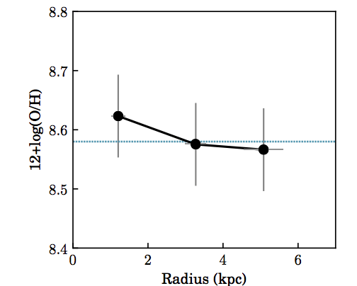
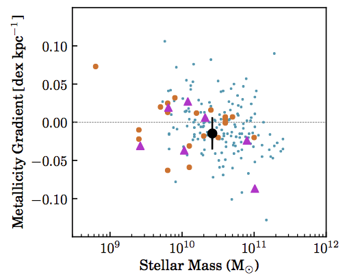
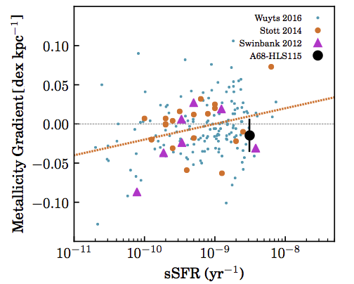
Figure 3 (top panel) shows the oxygen abundance gradient as a function of radius obtained using the N2 indicator. It has been derived at three different radii by fitting elliptical annuli on the velocity map in the source plane with the method of Krajnović et al. (2006). By averaging metallicity values of all the spaxels in the annuli, we obtain a slightly negative metallicity gradient (higher metallicity in the core than in outer regions) of dex in total (or dex kpc-1) although with a low significance. This is consistent with observations at high redshift which show generally flat or negative gradients (Jones et al., 2013; Stott et al., 2014, e.g.). However, it is now known that the spatial resolution and annular binning can have an impact on the obtained metallicity gradient (Yuan et al., 2013; Mast et al., 2014). Indeed, since our observations are seeing-limited and considering that the FWHM of the PSF varies between 1 and 5 kpc depending on the orientation, the observed metallicity gradient could be flattened by these effects. Using only three annuli to determine the gradient could also cause a flatter gradient.
Moreover, our metallicity gradient is similar to gradients found in galaxies with the same stellar mass and sSFR as shown in Fig. 3 (middle and bottom panels). We include data from Swinbank et al. (2012), Stott et al. (2014), and Wuyts et al. (2016), and the relation obtained by Stott et al. (2014) (in orange) for comparison. No correlation is seen with the stellar mass. However, Wang et al. (2017) observe a tentative anti-correlation between stellar mass and metallicity gradient, coherent with a scenario where more massive galaxies are more evolved. Stott et al. (2014) find a trend with the sSFR while combining their data with those of Rupke et al. (2010), Queyrel et al. (2012), and Swinbank et al. (2012), which could imply that the sSFR is driven by the amount of gas flowing towards the center. Using simulations, Sillero et al. (2017) find in a recent study that a correlation between the metallicity gradient and sSFR is seen in certain conditions when strong gas inflows are produced by interactions or instabilities. However, when adding the data from Wuyts et al. (2016), this trend becomes less obvious, which could mean that the gas flowing to the center might not be the only physical process that influences the sSFR.
5.3 Kinematics
Figure 4 (left panel) presents the velocity map in the source plane centered on the redshift obtained from the H emission line of the integrated spectrum. The map shows an obvious velocity gradient. To model the kinematics, we use a markov-chain Monte Carlo (MCMC) method to fit the observed velocity map with the PSF convolved model. We adopt the arctangent function for the velocity profile (Courteau, 1997), which has been used in many studies (e.g., Jones et al. 2010):
| (3) |
where is the radius, is the turnover radius, and is the maximum rotation velocity. All the parameters are free to vary when fitting the model. The fit is performed in the source plane. The model velocity map obtained is shown in Fig. 4 (middle panel) and the kinematic properties obtained are presented in Table 2.
The rotation curve determined from the reconstructed H velocity map in the source plane and from the kinematic model is presented in Fig. 5. The curve in red indicates the intrinsic rotation curve, corrected for the inclination. The rotation curve reveals a rotating disk typical of star-forming galaxies on the MS (e.g., Förster Schreiber et al. 2009; Wisnioski et al. 2015).
The observed velocity dispersion map is shown in Fig. 4 (right panel). The intrinsic velocity dispersion is measured in spaxels on the major axis in the outer region of the disk to avoid beam smearing as much as possible and is also corrected for the instrumental broadening following Eq. 2. From Burkert et al. (2016) and Johnson et al. (2018), we know that even if we take the measurement in the outer region, there is still an increase of the dispersion value due to the beam smearing, which is of - if we take into account the stellar mass and inclination of our galaxy. If we add this extra-correction for the beam smearing, we obtain an intrinsic velocity dispersion of km s-1 (Table 2). This value is in agreement with an evolution of the intrinsic velocity dispersion with redshift, where galaxies at high redshift show a higher intrinsic velocity dispersion compared to the local galaxies (Wisnioski et al., 2015; Turner et al., 2017; Girard et al., 2018, e.g.). This value is nevertheless higher compared to samples at and of Wisnioski et al. (2015), which show a mean dispersion of 25 and 50 km s-1, respectively. This suggests that the high turbulence observed in our galaxy could be due to the high gas fraction of of this source. Moreover, the observed velocity dispersion map does not show any evidence of a peak in the kinematic center. An increase of the velocity dispersion in the center can be an indication of a rotating disk according to Rodrigues et al. (2017). However, this increase is lower for galaxies with high velocity dispersion ( km s-1) and could explain why we do not see this effect here (Johnson et al., 2018).
We obtain a ratio , meaning that the galaxy is dominated by rotation if we use the typical criterion of (Wisnioski et al., 2015; Mason et al., 2017; Turner et al., 2017; Girard et al., 2018, e.g.), but this ratio also indicates that the disk is marginally stable. This value is typical at according to the stability () evolution relation with redshift obtained by Wisnioski et al. (2015), and our galaxy is in good agreement with the trends they find where the stability () is correlated to sSFR and . Indeed, they get a lower stability () at high sSFR () and (). This is fully in line with the , sSFR, and measured in A68-HLS115. This suggests that the disk turbulence and instability in this galaxy are mostly regulated by incoming gas (available gas reservoir for star formation).
Moreover, the Toomre stability criterion (Toomre, 1964) can be expressed as
| (4) |
We obtain for our galaxy a direct measurement of . A value of is expected for a thin quasi-stable gas disk and is an indication of an unstable system that can fragment into clumps (Jones et al., 2010, e.g.). However, the critical value of the Toomre parameter for a thick gas disk is (Kim & Ostriker, 2007), which could be the case of A68-HLS115 since several studies point out that disk galaxies at are thick (Genzel et al., 2011, e.g.). White et al. (2017) also obtain a linear correlation between and from Eq. 4. From this relation and assuming hydrostatic equilibrium and that the pressure is caused only by the turbulent motions of the gas, they find that a higher gas fraction leads to thicker disks in marginally stable disks.


5.4 Properties of the clumps
The H and [NII]/H maps of A68-HLS115 in the source plane are presented in Fig. 6. We are able to identify three clumps in the image plane of the H map with CLUMPFIND (Williams et al., 1994) using a selection criterion of . Overlaid on the observed HST/F814W images with dashed white lines (see Fig. 1), we see that these H clumps are blends of multiple smaller star-forming clumps resolved in the HST image. The H clumps are exclusively distributed over the eastern part of the galaxy, while no H clump is detected in the western part yet holding one of the most prominent HST clumps. When looking in the source plane after the reconstruction, we find that the H clumps as well as the clumps observed in the HST images could trace a spiral structure. This scenario would be consistent with the observed velocity map which is typical of a rotating disk.
| Parameters | Clump 1 | Clump 2 | Clump 3 |
|---|---|---|---|
| SFRHα a aa a aa The SFR has been corrected for lensing and for the dust attenuation using the extinction measured from the integrated spectrum. | |||
| Radius b bb b bb The radius corresponds to , where and are the semi-major and semi-minor axis. The typical error on the size of the clump is about . [kpc] | 1.57 | 1.34 | 1.26 |
| 12+log(O/H)N2 | |||
| 12+log(O/H)O3N2 | - | - | |
| 12+log(O/H)O3N2,Hα c cc c cc Since the H emission line is only detected in the clump 1, the H flux has been derived from the H flux using a H/H ratio of 2.86 and the measured from the integrated spectrum. | |||
| d dd d dd is the median dispersion value of the spaxels inside each clump. The errors correspond to 95% confidence range. |
We combine all the spaxels within each clump and obtain individual spectra. We fit the H and [NII] emission lines in the same way as the integrated spectrum (see Sect. 4.2) for each clump (see Fig. 7). For the brightest clump (clump 1), it is also possible to fit the [OIII] and H emission lines. As a result, we obtain the total flux of each emission line for each clump, the SFRHα assuming a uniform extinction correction derived from the integrated spectrum, the oxygen abundance using the N2 and O3N2 indicators from Pettini & Pagel (2004), for which we use the H flux to derive the H flux, and the velocity dispersion corrected for the instrumental broadening. Since the velocity dispersions can be affected by beam smearing, we also measure the median dispersion value per clump using the velocity dispersion map. Indeed, this effect is less important for the measurement of individual spaxels. The main properties of the clumps are summarized in Table 3.
We get a very similar metallicity for each clump using the N2 indicator, while using the O3N2 we get a value slightly lower for clump 2, but the difference is not significant. We also get a high velocity dispersion for our three clumps, with a difference of between clump 1 and 3. Overall, the clumps show a similar metallicity, a similar velocity dispersion as in the rest of the disk (see Table 2), and seem to be embedded in the rotating disk.
Livermore et al. (2015) show an evolution of the clump surface brightness with higher values at high redshift compared to local HII regions. The three clumps follow this trend with an SFRHα about times higher than what we find in the local Universe for clumps with similar size according to the relation obtained by Livermore et al. (2015) at using the SINGS survey (Kennicutt et al., 2003). We also find that the three clumps contribute individually to on the SFRHα of the whole galaxy. Therefore, the majority () of the observed flux is found outside these regions. Similarly, Guo et al. (2012) obtain SFRs of and for individual clumps and total contribution, respectively, for star-forming galaxies at with SFR measured through SED fitting.
For clump 1 we can measure the Balmer decrement (H/H=8) , which turns out to be higher than that measured from the integrated spectrum. The attenuation of clump 1 is therefore quite high, , showing that at least this clump does not correspond to a region which is visible due to inhomogeneities in the dust distribution, which could mimic stellar and ionized gas clumps, as suggested by Buck et al. (2017). We therefore conclude that this “clump" (region) does most likely indeed correspond to some physical concentration of ionized gas (HII region(s)), which is primarily powered by one or several young stellar clusters, and that such physical entities truly form in high-redshift galaxies.
6 Conclusions
We have presented new observations of A68-HLS115 at , a star-forming galaxy located behind the galaxy cluster Abell 68, but strongly lensed by a cluster galaxy member, with SINFONI, a NIR IFU at the VLT. We detect H, H, [NII], and [OIII] emission lines. Combined with images covering the B band to the FIR and CO(2-1) observations, this makes this galaxy one of the only sources for which such multi-band observations are available and for which it is possible to study the properties of resolved clumps and to perform a detailed analysis of the integrated properties, kinematics, and metallicity. This source is also one of the most gas-rich galaxies () known at .
A68-HLS115 is a dusty and gas-rich galaxy with a stellar mass M⊙ and a star formation rate SFR M⊙ yr-1, as measured from the UV, IR, and from SED fits (Table 1). Comparing the attenuation from Balmer decrement with that derived from the UV and IR luminosity, we find a higher attenuation for the nebular lines compared to the stellar continuum, as found for several other galaxies at high redshift (Yoshikawa et al., 2010; Shivaei et al., 2016, e.g.).
The galaxy shows a velocity map typical of rotating galaxies and we obtain a high intrinsic velocity dispersion of . The stability ratio of is characteristic of galaxies at high redshift with a high sSFR and gas fraction and suggests that the disk is marginally stable. We obtain a direct measurement of the Toomre stability criterion of , which could suggest the presence of a thick gas disk. We also find a slightly negative metallicity gradient.
We are able to identify three clumps in the H map that show similar metallicity and velocity dispersion to one another, but also to the host galaxy, and that seem embedded in the rotating disk. We obtain star formation rate densities approximately times higher than what is found for HII regions in the local Universe. Finally, the clumps in our galaxy represent of the SFRHα of the whole galaxy.
For one of the H clumps, we can measure the extinction from the Balmer decrement, finding an extinction which is higher than the average over the entire galaxy. This shows that at least this clump is not just an appearance caused by inhomogeneities in the dust distribution of the interstellar medium, as suggested by Buck et al. (2017) for the stellar or ionized gas clumps frequently observed at high redshift.
Acknowledgements.
This work was supported by the Swiss National Science Foundation. MG is grateful to the Fonds de recherche du Québec - Nature et Technologies (FRQNT) for financial support.References
- Adamo et al. (2013) Adamo, A., Östlin, G., Bastian, N., et al. 2013, ApJ, 766, 105
- Álvarez-Márquez et al. (2016) Álvarez-Márquez, J., Burgarella, D., Heinis, S., et al. 2016, A&A, 587, A122
- Bournaud et al. (2014) Bournaud, F., Perret, V., Renaud, F., et al. 2014, ApJ, 780, 57
- Buck et al. (2017) Buck, T., Macciò, A. V., Obreja, A., et al. 2017, MNRAS, 468, 3628
- Burkert et al. (2016) Burkert, A., Förster Schreiber, N. M., Genzel, R., et al. 2016, ApJ, 826, 214
- Cañameras et al. (2017) Cañameras, R., Nesvadba, N., Kneissl, R., et al. 2017, A&A, 604, A117
- Calzetti et al. (2000) Calzetti, D., Armus, L., Bohlin, R. C., et al. 2000, ApJ, 533, 682
- Cardelli et al. (1989) Cardelli, J. A., Clayton, G. C., & Mathis, J. S. 1989, ApJ, 345, 245
- Cava et al. (2018) Cava, A., Schaerer, D., Richard, J., et al. 2018, Nature Astronomy, 2, 76
- Chabrier (2003) Chabrier, G. 2003, PASP, 115, 763
- Courteau (1997) Courteau, S. 1997, AJ, 114, 2402
- Cowie et al. (1995) Cowie, L. L., Hu, E., & Songaila, A. 1995, AJ, 110, 1576
- Daddi et al. (2007) Daddi, E., Dickinson, M., Morrison, G., et al. 2007, ApJ, 670, 156
- De Barros et al. (2016) De Barros, S., Reddy, N., & Shivaei, I. 2016, ApJ, 820, 96
- Dekel et al. (2009) Dekel, A., Sari, R., & Ceverino, D. 2009, ApJ, 703, 785
- Dessauges-Zavadsky et al. (2017) Dessauges-Zavadsky, M., Schaerer, D., Cava, A., Mayer, L., & Tamburello, V. 2017, ApJ, 836, L22
- Dessauges-Zavadsky et al. (2015) Dessauges-Zavadsky, M., Zamojski, M., Schaerer, D., et al. 2015, A&A, 577, A50
- Dominguez et al. (2013) Dominguez, A., Siana, B., Henry, A. L., et al. 2013, ApJ, 763, 145
- Elmegreen et al. (2009) Elmegreen, B. G., Elmegreen, D. M., Fernandez, M. X., & Lemonias, J. J. 2009, ApJ, 692, 12
- Elmegreen et al. (2007) Elmegreen, D. M., Elmegreen, B. G., Ravindranath, S., & Coe, D. A. 2007, ApJ, 658, 763
- Förster Schreiber et al. (2009) Förster Schreiber, N. M., Genzel, R., Bouché, N., et al. 2009, ApJ, 706, 1364
- Förster Schreiber et al. (2011) Förster Schreiber, N. M., Shapley, A. E., Genzel, R., et al. 2011, ApJ, 739, 45
- Genzel et al. (2011) Genzel, R., Newman, S., Jones, T., et al. 2011, ApJ, 733, 101
- Girard et al. (2018) Girard, M., Dessauges-Zavadsky, M., Schaerer, D., et al. 2018, A&A, 613, A72
- Gray & Corbally (1994) Gray, R. O. & Corbally, C. J. 1994, AJ, 107, 742
- Guo et al. (2012) Guo, Y., Giavalisco, M., Ferguson, H. C., Cassata, P., & Koekemoer, A. M. 2012, ApJ, 757, 120
- Johnson et al. (2018) Johnson, H. L., Harrison, C. M., Swinbank, A. M., et al. 2018, MNRAS, 474, 5076
- Jones et al. (2013) Jones, T., Ellis, R. S., Richard, J., & Jullo, E. 2013, ApJ, 765, 48
- Jones et al. (2010) Jones, T. A., Swinbank, A. M., Ellis, R. S., Richard, J., & Stark, D. P. 2010, MNRAS, 404, 1247
- Kashino et al. (2013) Kashino, D., Silverman, J. D., Rodighiero, G., et al. 2013, ApJ, 777, L8
- Kennicutt (1998) Kennicutt, Jr., R. C. 1998, ARA&A, 36, 189
- Kennicutt et al. (2003) Kennicutt, Jr., R. C., Armus, L., Bendo, G., et al. 2003, PASP, 115, 928
- Kim & Ostriker (2007) Kim, W.-T. & Ostriker, E. C. 2007, ApJ, 660, 1232
- Krajnović et al. (2006) Krajnović, D., Cappellari, M., de Zeeuw, P. T., & Copin, Y. 2006, MNRAS, 366, 787
- Kurucz (1993) Kurucz, R. L. 1993, VizieR Online Data Catalog, 6039
- Leethochawalit et al. (2016) Leethochawalit, N., Jones, T. A., Ellis, R. S., et al. 2016, ApJ, 820, 84
- Livermore et al. (2012) Livermore, R. C., Jones, T., Richard, J., et al. 2012, MNRAS, 427, 688
- Livermore et al. (2015) Livermore, R. C., Jones, T. A., Richard, J., et al. 2015, MNRAS, 450, 1812
- Mandelker et al. (2017) Mandelker, N., Dekel, A., Ceverino, D., et al. 2017, MNRAS, 464, 635
- Mason et al. (2017) Mason, C. A., Treu, T., Fontana, A., et al. 2017, ApJ, 838, 14
- Mast et al. (2014) Mast, D., Rosales-Ortega, F. F., Sánchez, S. F., et al. 2014, A&A, 561, A129
- Patrício et al. (2018) Patrício, V., Richard, J., Carton, D., et al. 2018, MNRAS, 477, 18
- Pettini & Pagel (2004) Pettini, M. & Pagel, B. E. J. 2004, MNRAS, 348, L59
- Price et al. (2014) Price, S. H., Kriek, M., Brammer, G. B., et al. 2014, ApJ, 788, 86
- Puglisi et al. (2017) Puglisi, A., Daddi, E., Renzini, A., et al. 2017, ApJ, 838, L18
- Queyrel et al. (2012) Queyrel, J., Contini, T., Kissler-Patig, M., et al. 2012, A&A, 539, A93
- Reddy et al. (2010) Reddy, N. A., Erb, D. K., Pettini, M., Steidel, C. C., & Shapley, A. E. 2010, ApJ, 712, 1070
- Reddy et al. (2015) Reddy, N. A., Kriek, M., Shapley, A. E., et al. 2015, ApJ, 806, 259
- Richard et al. (2007) Richard, J., Kneib, J.-P., Jullo, E., et al. 2007, ApJ, 662, 781
- Richard et al. (2010) Richard, J., Smith, G. P., Kneib, J.-P., et al. 2010, MNRAS, 404, 325
- Rodighiero et al. (2010) Rodighiero, G., Cimatti, A., Gruppioni, C., et al. 2010, A&A, 518, L25
- Rodrigues et al. (2017) Rodrigues, M., Hammer, F., Flores, H., Puech, M., & Athanassoula, E. 2017, MNRAS, 465, 1157
- Rupke et al. (2010) Rupke, D. S. N., Kewley, L. J., & Chien, L.-H. 2010, ApJ, 723, 1255
- Salmi et al. (2012) Salmi, F., Daddi, E., Elbaz, D., et al. 2012, ApJ, 754, L14
- Salpeter (1955) Salpeter, E. E. 1955, ApJ, 121, 161
- Schaerer et al. (2013) Schaerer, D., de Barros, S., & Sklias, P. 2013, A&A, 549, A4
- Shivaei et al. (2016) Shivaei, I., Kriek, M., Reddy, N. A., et al. 2016, ApJ, 820, L23
- Sillero et al. (2017) Sillero, E., Tissera, P. B., Lambas, D. G., & Michel-Dansac, L. 2017, MNRAS, 472, 4404
- Sklias et al. (2014) Sklias, P., Zamojski, M., Schaerer, D., et al. 2014, A&A, 561, A149
- Stott et al. (2014) Stott, J. P., Sobral, D., Swinbank, A. M., et al. 2014, MNRAS, 443, 2695
- Swinbank et al. (2011) Swinbank, A. M., Papadopoulos, P. P., Cox, P., et al. 2011, ApJ, 742, 11
- Swinbank et al. (2012) Swinbank, A. M., Smail, I., Sobral, D., et al. 2012, ApJ, 760, 130
- Tamburello et al. (2015) Tamburello, V., Mayer, L., Shen, S., & Wadsley, J. 2015, MNRAS, 453, 2490
- Tamburello et al. (2017) Tamburello, V., Rahmati, A., Mayer, L., et al. 2017, MNRAS, 468, 4792
- Toomre (1964) Toomre, A. 1964, ApJ, 139, 1217
- Turner et al. (2017) Turner, O. J., Cirasuolo, M., Harrison, C. M., et al. 2017, MNRAS, 471, 1280
- Wang et al. (2017) Wang, X., Jones, T. A., Treu, T., et al. 2017, ApJ, 837, 89
- White et al. (2017) White, H. A., Fisher, D. B., Murray, N., et al. 2017, ApJ, 846, 35
- Williams et al. (1994) Williams, J. P., de Geus, E. J., & Blitz, L. 1994, ApJ, 428, 693
- Wisnioski et al. (2015) Wisnioski, E., Förster Schreiber, N. M., Wuyts, S., et al. 2015, ApJ, 799, 209
- Wisnioski et al. (2012) Wisnioski, E., Glazebrook, K., Blake, C., et al. 2012, MNRAS, 422, 3339
- Wuyts et al. (2012) Wuyts, E., Rigby, J. R., Gladders, M. D., et al. 2012, ApJ, 745, 86
- Wuyts et al. (2016) Wuyts, E., Wisnioski, E., Fossati, M., et al. 2016, ApJ, 827, 74
- Wuyts et al. (2013) Wuyts, S., Förster Schreiber, N. M., Nelson, E. J., et al. 2013, ApJ, 779, 135
- Yoshikawa et al. (2010) Yoshikawa, T., Akiyama, M., Kajisawa, M., et al. 2010, ApJ, 718, 112
- Yuan et al. (2013) Yuan, T.-T., Kewley, L. J., & Rich, J. 2013, ApJ, 767, 106