Blind Ptychography by Douglas-Rachford Splitting

Our reconstruction scheme is based on alternating minimization with the Douglas-Rachford splitting (DRS) method. DRS is a proximal point method closely related to the Alternating Direction Method of Multipliers (ADMM). The existing theory and analysis for DRS and ADMM (see, e.g. [29, 11, 18, 16]) are limited to the convex optimization, except for a few exceptions (see e.g. [5, 28, 21]). In particular, the performance of DRS and ADMM in the non-convex setting depends sensitively on the choice of the objective functions as well as the selection of the relaxation parameters and the step size which are the main focus of our proposed scheme.

Our choices of the objective functions and the step size are informed by the uniqueness theory [12], the Poisson noise model and the stability analysis. The confluence of the three considerations leads to the proposed scheme (acronym AMDRS). The crux of our stability analysis (Proposition 2.1 and 2.2) is that the true solution (modulo the scaling factor and the affine phase ambiguity) to blind ptychography are stable fixed points of AMDRS with any step size and, moreover, in the case of the unit step size, all other fixed points are saddle points. This suggests that a unit step size is a good choice for AMDRS in contrast to (sufficiently) small step sizes typically required for nonconvex convergence analysis [28, 21].

For any iterative scheme for non-convex optimization, the initialization of the iteration plays a crucial role in the convergence of the scheme. The initialization step is often glossed over in the development of numerical schemes due to lack of a good metric (see e.g. [31, 56, 50]). In our numerical experiments, PPC turns out to be an excellent initialization method and metric for controlling the convergence behavior of the schemes. In particular, our schemes converge globally and geometrically under PPC with $\delta=1/2$.

In additional to demonstrate the numerical performance of the proposed schemes, we propose a special boundary condition (the bright-field boundary condition) to remove the linear phase ambiguity. The capability of removing the linear phase ambiguity is particularly important for 3D blind tomography as the different linear phase ramps for different projections would collectively create enormous 3D ambiguities that are difficult to make consistent.

The rest of the paper is organized as follows. In Section 2, we introduce the Douglas-Rachford splitting method as the key ingredient of our reconstruction algorithms, Gaussian-DRS and Poisson-DRS. We give the fixed point analysis in Section 2.3. In Section 3, we perform numerical experiments with our schemes. In Appendix A, we show that Gaussian-DRS is an asymptotic form of Poisson-DRS. We conclude in Section 4.

A main feature of alternating minimization scheme is the monotonicity property:

We consider two log-likelihood cost functions [52, 2] for noise-robustness

based on the maximum likelihood principle for the Poisson noise model. The Poisson log-likelihood function (4) is asymptotically reduced to (5) as shown in Appendix A.

The ptychographic iterative engines, PIE [44], ePIE [33] and rPIE [31], are both derived from the amplitude-based cost function (5). The maximum likelihood scheme is also a variance stabilization scheme which uniformizes the probability distribution for every pixel regardless of the measured intensity value [26]. It is well established that the amplitude-based cost function (5) outperforms the intensity-based cost function ${1\over 2}\||y|^{2}-b^{2}\|_{2}^{2}$ [56]. See [19, 59] for more choices of objective functions.

For non-convex iterative optimization, a good initial guess or some regularization is usually crucial for convergence [52, 2]. We assume that the initial guess for the probe satisfies PPC. To test the linear phase ambiguity, we also consider the probe initialization

where $\phi({\mathbf{n}})$ are independently and uniformly distributed on $(-\delta\pi,\delta\pi)$. We use $\delta\in[0,1/2]$ as the control parameter for the proximity of the initial probe to the true probe, modulo a linear phase factor represented by ${\mathbf{k}}$, and denote this class of probe initialization by PPC(${\mathbf{k}},\delta$).

We formulate the inner loops (Step 2 and 3 in Algorithm 1) of AM as

where the additional objective function $K$ enforces the constraint that $u$ is in the range of $A_{k}$ or $B_{k}$.

We solve (7) by the Douglas-Rachford splitting (DRS) method which is a proximal point algorithm for minimizing a sum of two objective functions [29, 11]. This is motivated by the good performance of the classical Douglas-Rachford (CDR) algorithm [9, 29] (aka the difference map [10] in the optics literature), a special case of DRS with an infinitely large step size, which has been used for ptychographic reconstruction [51, 50, 55] and analyzed in [5, 6]. The CDR iteration, however, exhibits only a sub-linear convergence globally in the noiseless case [5] and, when the optimization problems become infeasible (e.g. with noisy data), tends to fluctuate and underperform, hence the search for a faster convergent and more robust DRS.

DRS is defined by the following iteration for $l=1,2,3\cdots$

where $\hbox{prox}_{{\mathcal{L}}/\rho}(u^{k}):=\mathop{\text{argmin}}\limits_{x}{\mathcal{L}}(x)+\frac{\rho}{2}\|x-u^{k}\|^{2}$. For the initial guess $u^{1}_{1}$ in our simulations, we let $u^{1}_{1}=A_{1}^{*}f_{1}$ where $f_{1}({\mathbf{n}})$ is a phase object with i.i.d. phase uniformly distributed over $[0,2\pi]$ or a constant value 0. Here $\gamma=1/\rho$ is often referred to as the step size of DRS.

It can be checked that DRS (7) is formally equivalent to the Alternating Direction Method of Multipliers (ADMM)

Our choice of $K$ is important to our implementation of DRS. Since the object estimate in the $k-$th epoch must be of the form $A_{k}g$ for some $g\in\mathbb{C}^{n\times n}$, we let $K(u)$ be the indicator function $\chi_{k}(u)$ of the range of $A_{k}$, i.e. $\chi_{k}(u)=0$ if $y$ is in the range of $A^{*}_{k}$; and $\chi_{k}(u)=\infty$ otherwise. For this choice of $K$, $\hbox{prox}_{K/\rho}(u)=P_{k}u$ is independent of $\rho$. This should be contrasted with the choice of the distance function adopted in [28] for the tractability of the convergence analysis due to the smoothness of the distance function.

For the Gaussian case (5), we update the object estimate as

where $u_{k}^{\infty}$ is the terminal output of the following iteration

Substituting (10) and (11) into (12) and reorganizing the resulting equation, we obtain

where $P_{k}=A_{k}A_{k}^{\dagger}$ is the orthogonal projection onto the range of $A_{k}$ and $R_{k}=2P_{k}-I$ is the corresponding reflector.

Likewise, we update the probe as

where $v_{k}^{\infty}$ is the terminal output of the following iteration

where $Q_{k}=B_{k}B_{k}^{\dagger}$ is the orthogonal projection onto the range of $B_{k}$ and $S_{k}$ the corresponding reflector.

For the Poisson case (4), the inner loops take a more complicated form

After the inner loops terminate, we update the object and probe as (9) and (14),respectively.

We shall refer to DRS with the Poisson log-likelihood function (16)-(17) and the Gaussian version (13)-(15) by the acronyms Poisson-DRS and Gaussian-DRS, respectively. We call the the two algorithms the Alternating Minimization with Douglas-Rachford Splitting (AMDRS). Due to the non-differentiability of both $K$ and ${\mathcal{L}}$, the global convergence property of the proposed DRS method is beyond the current framework of analysis [28].

In the limiting case of $\rho\to 0$, both Gaussian-DRS and Poisson-DRS become the classical Douglas-Rachford algorithm.

The computation involved in Gaussian-DRS and Poisson-DRS are mostly pixel-wise operations (hence efficient) except for the pseudoinverses $A_{k}^{\dagger}=(A^{*}_{k}A_{k})^{-1}A^{*}_{k}$ and $B_{k}^{\dagger}=(B^{*}_{k}B_{k})^{-1}B^{*}_{k}$. In blind ptychography, due to the isometry of the Fourier transform, $A^{*}_{k}A_{k}$ and $B^{*}_{k}B^{\dagger}_{k}$ are diagonal matrices and easy to invert [12].

For simplicity, we shall focus the stability analysis on the fixed points of Gaussian DRS.

Suppose that the limit $(u,v)=\lim_{k,l\to\infty}(u_{k}^{l},v_{k}^{l})$ exist where $(u^{l}_{k},v^{l}_{k})$ are two-parameter arrays of the Gaussian-DRS iterates. Let $\lim_{k\to\infty}A_{k}=A_{\infty},\ \lim_{k\to\infty}B_{k}=B_{\infty}$.

Let $P_{\infty}=A_{\infty}A_{\infty}^{\dagger}$ and $Q_{\infty}=B_{\infty}B_{\infty}^{\dagger}$ denote the orthogonal projection onto the range of $A_{\infty}$ and $B_{\infty}$, respectively. Let $P^{\perp}_{\infty}=I-P_{\infty}$ and $Q^{\perp}_{\infty}=I-Q_{\infty}$ denote the orthogonal complements of $P_{\infty}$ and $Q_{\infty}$, respectively. Denote $R_{\infty}=2P_{\infty}-I,S_{\infty}=2Q_{\infty}-I$.

Passing to the limit in (13)-(15) we obtain the fixed point equation for Gaussian-DRS

It is straightforward to check that the true solution ($u_{0}:={\mathcal{F}}(\mu,f),v_{0}:={\mathcal{F}}(\mu,f)$) is a fixed point of Gaussian-DRS (13)-(15) and Poisson-DRS (16)-(17).

We now give theoretical motivation for our numerical choice of $\rho=1$.

For a solution $(u,v)$ to the fixed point equation (18)-(19), define the reflection images, $x:=R_{\infty}u,\,\,y:=S_{\infty}v.$ Denote the right hand side of (18) as $U(x)$ and consider a perturbation of $x$ by $\epsilon z$ where $\epsilon$ is a small positive number. Set ${\Omega}=\hbox{\rm diag}(\mbox{\rm sgn}(x))$, $C={\Omega}^{*}A_{\infty}$, $\eta={\Omega}^{*}z$. Suppose $|x|>0$. From somewhat tedious but straightforward calculation, we have

where

The differential $J_{B}$ of the right hand side of (19) has the similar structure.

We prove the following results in Appendix B and C. The first result says that for $\rho=1$ all the non-solution fixed points are linearly unstable and the second says that for $\rho\in[0,\infty)$ the true solutions to blind ptychography are stable fixed points.

Moreover, under the uniqueness conditions of [12], Proposition 2.1 and 2.2 then imply that the true solution and its inherent ambiguities (modulo a scaling factor and affine phase ramp) are the only stable fixed points of Gaussian-DRS with the unit step size. Therefore Gaussian-DRS with the unit step size should not stagnate near a fixed point that is not a solution to blind ptychography.

Our first test image is 256-by-256 Cameraman+ ${\rm i}$ Barbara (CiB). The resulting test object has the phase range $\pi/2$. The second test object is randomly-phased phantom (RPP) defined by $f_{*}=P\odot e^{{\rm i}\phi}$ where $P$ is the standard phantom (Fig. 3(a)) and $\{\phi({\mathbf{n}})\}$ are i.i.d. uniform random variables over $[0,2\pi]$. RPP has the maximal phase range because of its noise-like phase profile. In addition to the huge phase range, RPP has loosely supported parts with respect to the measurement schemes (see below) due to its thick dark margins around the oval.

We do not explore the issue of varying the probe size in the present work, which has been done with the classical Douglas-Rachford algorithm in [6]. We fix the probe size to $60\times 60$. In addition to the i.i.d. probe, we consider also correlated probe produced by convolving the i.i.d. probe with characteristic function of the set $\{(k_{1},k_{2})\in\mathbb{Z}^{2}:\max\{|k_{1}|,|k_{2}|\}\leq c\cdot m;\ c\in(0,1]\}$ where the constant $c$ is a measure of the correlation length in the unit of $m=60$ (Fig. 4).

We let $\delta_{k}^{1}$ and $\delta^{2}_{l}$ in the rank-one scheme (1) and $\delta_{kl}^{1}$ and $\delta^{2}_{kl}$ in the full-rank scheme (2) to be i.i.d. uniform random variables over $\llbracket-4,4\rrbracket$. In other words, the adjacent probes overlap by an average of $\tau/m=50\%$.

We use relative error (RE) and relative residual (RR) as the merit metrics for the recovered image $f_{k}$ and probe $\mu_{k}$ at the $k^{th}$ epoch:

Note that in (22) the linear phase ambiguity is discounted along with a scaling factor.

First we compare performance of AMDRS with different combinations of objective functions, scanning schemes and random probes in the case of noiseless measurements with the periodic boundary condition. We use the stopping criteria for the inner loops:

with the maximum number of iterations capped at 60.

Figure 5 shows geometric decay of RE (22) at various rates $r_{o}$ for the test object CiB. In particular, Fig. 5(a) shows that the full-rank scheme outperforms the rank-one scheme and that Poisson-DRS outperforms (slightly) Gaussian-DRS while Figure 5(b) shows that the i.i.d. probe yields the smallest rate of convergence ($r_{o}=0.7562$) closely followed by the rate ($r_{o}=0.7583$) for $c=0.4$.

For noisy measurement, the level of noise is measured in terms of the noise-to-signal ratio (NSR).

Figure 6 shows RE (22) for CiB versus NSR for Poisson-DRS and Gaussian-DRS with the periodic boundary condition, i.i.d. probe and the full-rank scheme. The maximum number of epoch in AMDRS is limited to $100$. The RR stabilizes usually after 30 epochs. The (blue) reference straight line has slope 1. We see that the Gaussian-DRS outperforms the Poisson-DRS, especially when the Poisson RE becomes unstable for NSR $\geq 35\%$. As noted in [31, 61, 7] fast convergence (with the Poisson log-likelihood function) may introduce noisy artifacts and reduce reconstruction quality.

For the rest of the experiments, we use noiseless data, Poisson-DRS and the full-rank scheme.

When the probe steps outside of the boundary of the object domain, the area ${\mathcal{M}}\setminus\mathbb{Z}_{n}^{2}$ needs special treatment in the reconstruction process.

The periodic boundary condition conveniently treats all diffraction patterns and object pixels in the same way by assuming that $\mathbb{Z}_{n}^{2}$ is a (discrete) torus. The periodic boundary condition generally forces the slope $\mathbf{r}$ in the linear phase ambiguity to be integers. The dark-field and bright-field boundary conditions assume zero and nonzero values, respectively, in ${\mathcal{M}}\setminus\mathbb{Z}_{n}^{2}$.

Depending on our knowledge of the boundary values, we may or may not enforce the boundary condition in each case. When the bright-field boundary condition is enforced, the linear phase ambiguity disappears from the object estimate. On the contrary, enforcing the dark-field boundary condition can not remove the linear phase ambiguity. In both cases, however, enforcing either boundary condition speeds up the convergence as shown in Figure 7 which is produced by keeping the maximum iterations of the inner loops to 30.

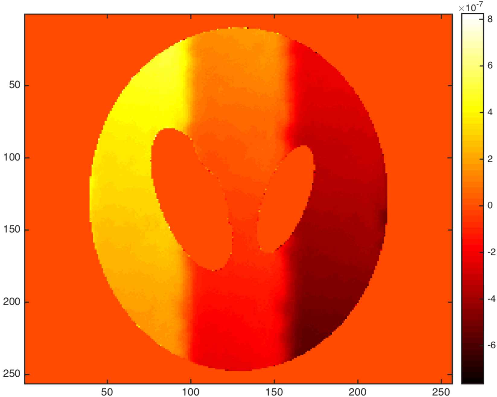
Moreover, the dark-field boundary condition can pose a challenge for reconstruction if the object domain has many dark pixels as in the case of RPP. Fig. 8(a) shows an example of failed reconstruction with PPC(0,0,0.5) of RPP which has a piece of the shell shifted sideway. Two ways to fix the problem: One is to improve the initialization condition and the other is to use a different boundary conditions (periodic or bright-field BC). Fig. 8(b) shows the reconstructed phase error with the periodic BC (note the scale of the color bar). Fig. 7(b) shows the relative error with probe initialization PPC(0, 0, 0.4) and various boundary conditions.

To show that the linear phase ambiguity is absent under the bright-field boundary condition, we test AMDRS with the initialization PPC$(-0.5,0.5,{1\over 2})$ and use a more stringent error metric

Note that PPC$(-0.5,0.5,{1\over 2})$ violates the probe phase constraint $\Re(\bar{\nu}^{0}\odot\mu^{0})>0$ allowed by the uniqueness theory. The linear phase factor is introduced in the initialization to test if it persists in the reconstruction.

We also use the less tolerant stopping rule

for the inner loops with the maximum number of iteration capped at 80, the rate of convergence accelerates.

Fig. 9 demonstrates the capability of the bright-field boundary condition to eliminate the linear phase ambiguity as the stronger error metric (24) decays geometrically before settling down to the final level of accuracy. The higher boundary value ($255$ in Fig. 9(a)) leads to faster convergence than the lower boundary value ($100$ in Fig. 9(b)). The final level of accuracy, however, depends on how accurately the inner loops for each epoch are solved. For example, increasing the maximum number of iteration from 80 to 110, significantly enhances the final accuracy of reconstruction (not shown).

References

- [1] B. Abbey, K. A. Nugent, G. J. Williams, J.N. Clark, A.G. Peele , M.A. Pfeiffer, M. De Jonge & I. McNulty, “Keyhole coherent diffractive imaging.” Nat. Phys. 4 (2008) 394-398.
- [2] L. Bian, J. Suo, J. Chung, X. Ou, C. Yang, F. Chen, and Q. Dai, “Fourier ptychographic reconstruction using Poisson maximum likelihood and truncated Wirtinger gradient,” Sci. Rep. 6 (2016), 27384.
- [3] O. Bunk, M. Dierolf, S. Kynde, I. Johnson, O. Marti, F. Pfeiffer, “Influence of the overlap parameter on the convergence of the ptychographical iterative engine,” Ultramicroscopy 108 (5) (2008) 481-487.
- [4] H.N. Chapman & K.A. Nugent, “Coherent lensless X-ray imaging,” Nat. Photon. 4 (2010) 833-839.
- [5] P. Chen and A. Fannjiang, “Phase retrieval with a single mask by Douglas-Rachford algorithms,” Appl. Comput. Harmon. Anal. 44 (2018), 665-699.
- [6] P. Chen and A. Fannjiang, “ Coded-aperture ptychography: uniqueness and reconstruction”, Inverse Problems 34 (2018) 025003.
- [7] P. Chen, A. Fannjiang and G. Liu, “Phase retrieval with one or two coded diffraction patterns by alternating projection with the null initialization,” J. Fourier Anal. Appl. 24 (2018), 719-758.
- [8] M. Dierolf, A. Menzel, P. Thibault, P. Schneider, C. M. Kewish, R. Wepf, O. Bunk, and F. Pfeiffer, “ Ptychographic x-ray computed tomography at the nanoscale,” Nature 467 (2010), 436-439.
- [9] J. Douglas and H.H. Rachford, ”On the numerical solution of heat conduction problems in two and three space variables,” Trans. Am. Math. Soc.82 (1956), 421-439.
- [10] V. Elser, “Phase retrieval by iterated projections,” J. Opt. Soc. Am. A 20 (2003), 40-55.
- [11] J. Eckstein and D.P. Bertsekas, “On the Douglas-Rachford splitting method and the proximal point algorithm for maximal monotone operators,” Math. Program. A 55 (1992), 293-318.
- [12] A. Fannjiang & P. Chen, “Blind ptychography: uniqueness and ambiguities,” arXiv:1806.02674.
- [13] A. Fannjiang and W. Liao, “Fourier phasing with phase-uncertain mask,” Inverse Problems 29 (2013) 125001.
- [14] H.M.L. Faulkner and J.M. Rodenburg, “Movable aperture lensless transmission microscopy: A novel phase retrieval algorithm,” Phys. Rev. Lett.93 (2004), 023903.
- [15] H.M.L. Faulkner and J.M. Rodenburg, “Error tolerance of an iterative phase retrieval algorithm for moveable illumination microscopy,” Ultramicroscopy 103:2 (2005), 153-164.
- [16] D. Gabay and B. Mercier. A dual algorithm for the solution of nonlinear variational problems via finite element approximation. Computers & Mathematics with Applications 2(1) (1976), 17-40.
- [17] S. Gao, P. Wang, F. Zhang, G. T. Martinez, P. D. Nellist, X. Pan & A. I. Kirkland, “Electron ptychographic microscopy for three-dimensional imaging,” Nat. Comm. 18(2017) 163.
- [18] R. Glowinski and A. Marroco. “Sur l’approximation, par éléments finis d’ordre un, et la résolution, par pénalisation-dualité d’une classe de problémes de dirichlet non linéaires,” ESAIM: Mathematical Modelling and Numerical Analysis, 9(1975), 41-76.
- [19] P. Godard, M. Allain, V. Chamard, and J. Rodenburg, “Noise models for low counting rate coherent diffraction imaging,” Opt. Express 20 (2012), 25914-25934.
- [20] M. Guizar-Sicairos, J.R. & Fienup, “Phase retrieval with transverse translation diversity: a nonlinear optimization approach.” Opt. Express 16 (2008), 7264-7278.
- [21] R. Hesse, D. R. Luke, S. Sabach, and M.K. Tam, “Proximal heterogeneous block implicit-explicit method and application to blind ptychographic diffraction imaging,” SIAM J. Imag. Sci. 8 (2015) pp. 426-457.
- [22] R. Horisaki, R. Egami & J. Tanida, “Single-shot phase imaging with randomized light (SPIRaL)”. Opt. Express 24 (2016), 3765-3773.
- [23] X. Huang, H. Yang, R. Harder, Y. Hwu, I.K. Robinson & Y.S. Chu,“Optimization of overlap uniformness for ptychography,” Opt. Express 22 (2014), 12634-12644.
- [24] Y. Jiang, Z. Chen, Y. Han, P. Deb, H. Gao, S. Xie, P. Purohit, M. W. Tate, J. Park, S. M. Gruner, V. Elser & D. A. Muller “Electron ptychography of 2D materials to deep sub-angstrom resolution,” Nature 559 (2018) 343-349.
- [25] C. Kohler, F. Zhang and W. Osten, “Characterization of a spatial light modulator and its application in phase retrieval,” Appl. Opt. 48 (2009) 4003-4008.
- [26] A.P. Konijnenberg, W.M.J. Coene and H.P. Urbach, “Model-independent noise-robust extension of ptychography,” Opt. Exp.26 (2018) 5857-5874.
- [27] C. Kuang, Y. Ma, R. Zhou, J. Lee, G. Barbastathis, R. R. Dasari, Z. Yaqoob & P.T.C. So, “Digital micromirror device-based laser-illumination Fourier ptychographic microscopy,” Opt. Exp. 23(2015), 26999-27010.
- [28] G. Li & T. K. Pong, “DouglasÐRachford splitting for nonconvex optimization with application to nonconvex feasibility problems,” Math. Program. A 159 (2016), 371-401
- [29] P.-L. Lions and B. Mercier,“Splitting algorithms for the sum of two nonlinear operators,” SIAM J. Num. Anal. 16 (1979), 964-979.
- [30] A. M. Maiden, M. J. Humphry, F. Zhang and J. M. Rodenburg, “Superresolution imaging via ptychography,” J. Opt. Soc. Am. A 28 (2011), 604-612.
- [31] A. M. Maiden, D. Johnson and P. Li, “Further improvements to the ptychographical iterative engine,” Optica 4 (2017), 736-745.
- [32] A.M. Maiden, G.R. Morrison, B. Kaulich, A. Gianoncelli & J.M. Rodenburg, “Soft X-ray spectromicroscopy using ptychography with randomly phased illumination,” Nat. Commun. 4 (2013), 1669.
- [33] A.M. Maiden & J.M. Rodenburg, “An improved ptychographical phase retrieval algorithm for diffractive imaging,” Ultramicroscopy 109 (2009), 1256-1262.
- [34] A. M. Maiden, J. M. Rodenburg and M. J. Humphry, “Optical ptychography: a practical implementation with useful resolution,” Opt. Lett. 35 (2010), 2585-2587.
- [35] G.R. Morrison, F. Zhang, A. Gianoncelli and I.K. Robinson, “X-ray ptychography using randomized zone plates,” Opt. Exp. 26 (2018) 14915-14927.
- [36] Y. S. G. Nashed, D. J. Vine, T. Peterka, J. Deng, R. Ross and C. Jacobsen, “Parallel ptychographic reconstruction,” Opt. Express 22 (2014) 32082-32097.
- [37] P.D. Nellist, B.C. McCallum & J.M. Rodenburg, “Resolution beyond the information limit in transmission electron microscopy, ” Nature 374 (1995) 630-632.
- [38] P.D. Nellist and J.M. Rodenburg, “ Electron ptychography. I. Experimental demonstration beyond the conventional resolution limits,” Acta Cryst. A 54 (1998), 49-60.
- [39] K.A. Nugent, “Coherent methods in the X-ray sciences, ” Adv. Phys.59 (2010) 1-99.
- [40] X. Ou, G. Zheng and C. Yang, “Embedded pupil function recovery for Fourier ptychographic microscopy,” Opt. Exp. 22 (2014) 4960-4972.
- [41] X. Peng, G.J. Ruane, M.B. Quadrelli & G.A. Swartzlander, “ Randomized apertures: high resolution imaging in far field,” Opt. Express 25 (2017) 296187.
- [42] F. Pfeiffer, “X-ray ptychography,” Nat. Photon. 12 (2017) 9-17.
- [43] J.M. Rodenburg, “Ptychography and related diffractive imaging methods,” Adv. Imaging Electron Phys. 150 (2008) 87-184.
- [44] J.M. Rodenburg and H.M.L. Faulkner, “A phase retrieval algorithm for shifting illumination”. Appl. Phys. Lett. 85 (2004), 4795.
- [45] M.H. Seaberg, A. d’Aspremont & J.J. Turner, “Coherent diffractive imaging using randomly coded masks,” Appl. Phys. Lett. 107 (2015) 231103.
- [46] P. Sidorenko, O. Lahav, Z. Avnat & O. Cohen, “Ptychographic reconstruction algorithm for frequency-resolved optical gating: super-resolution and supreme robustness,” Optica 3 (2016) 1320-1330.
- [47] J.C. Silva and A. Menzel, “Elementary signals in ptychography,” Opt. Exp. 23 (2015) 33812-33821.
- [48] M. Stockmar, P. Cloetens, I. Zanette, B. Enders, M. Dierolf, F. Pfeiffer, and P. Thibault,“Near-field ptychography: phase retrieval for inline holography using a structured illumination,” Sci. Rep. 3 (2013), 1927.
- [49] D. Sylman, V. Micó, J. Garca & Z. Zalevsky, “Random angular coding for superresolved imaging,” Appl. Opt.49 (2010), 4874-4882.
- [50] P. Thibault, M. Dierolf, O. Bunk, A. Menzel, F. Pfeiffer, “Probe retrieval in ptychographic coherent diffractive imaging,” Ultramicroscopy 109 (2009), 338-343.
- [51] P. Thibault, M. Dierolf, A. Menzel, O. Bunk, C. David, F. Pfeiffer, “High-resolution scanning X-ray diffraction microscopy”, Science 321 (2008), 379-382.
- [52] P. Thibault and M. Guizar-Sicairos, “ Maximum-likelihood refinement for coherent diffractive imaging”. New J. Phys. 14 (2012), 063004.
- [53] L. Tian, Z. Liu, L-H Yeh, M. Chen, J. Zhong, L. Waller, “Computational illumination for high-speed in vitro Fourier ptychographic microscopy,” Optica 2 (2015) 904-911.
- [54] L. Valzania, T. Feurer, P. Zolliker & E. Hack, “Terahertz ptychography,” Opt. Lett. 43 (2018), 543-546.
- [55] Z. Wen, C. Yang, X. Liu and S. Marchesini, “Alternating direction methods for classical and ptychographic phase retrieval,” Inverse Problems 28 (2012), 115010.
- [56] L. Yeh, J. Dong, J. Zhong, L.Tian, M. Chen, G. Tang, M. Soltanolkotabi, and L. Waller, “Experimental robustness of Fourier ptychography phase retrieval algorithms,” Optics Express 23 (2015) 33214-33240.
- [57] F. Zhang, B. Chen, G. R. Morrison, J. Vila-Comamala, M. Guizar-Sicairos & I. K. Robinson, “Phase retrieval by coherent modulation imaging,” Nat. Comm. 7 (2016):13367.
- [58] F. Zhang, G. Pedrini & W. Osten, “Phase retrieval of arbitrary complex-valued fields through aperture-plane modulation,” Phys. Rev. A 75 (2007), 043805.
- [59] Y. Zhang, P. Song, Q. Dai, “Fourier ptychographic microscopy using a generalized Anscombe transform approximation of the mixed Poisson-Gaussian likelihood,” Opt. Exp. 25 (2017) 168-179.
- [60] G. Zheng, R. Horstmeyer and C.Yang, “Wide-field, high-resolution Fourier ptychographic microscopy,” Nature Photonics 7 (2013), 739-745.
- [61] C. Zuo, J. Sun and Q. Chen, “Adaptive step-size strategy for noise-robust Fourier ptychographic microscopy,” Optics Express 24 (2016), 20724-20744.