跳到论文正文
W Papers独立论文阅读器 arXiv:1809.00959 论文正文 计算阅读时间 · 0%
引用这篇论文根据当前论文元数据生成,正式投稿前建议核对。


License: arXiv.org perpetual non-exclusive license
arXiv:1809.00959v2 [cs.PL] 19 Jan 2019

Translating Xd-C Programs to MSVL Programs

Meng Wang    Cong Tian Corresponding author: Corresponding authors: Cong Tian (ctian@mail.xidian.edu.cn), Nan Zhang (nanzhang@xidian.edu.cn) and Zhenhua Duan (zhhduan@mail.xidian.edu.cn). This research is supported by the National Natural Science Foundation of China under Grant Nos. 61420106004, 61732013 and 61751207.    Nan Zhang Corresponding author: Corresponding authors: Cong Tian (ctian@mail.xidian.edu.cn), Nan Zhang (nanzhang@xidian.edu.cn) and Zhenhua Duan (zhhduan@mail.xidian.edu.cn). This research is supported by the National Natural Science Foundation of China under Grant Nos. 61420106004, 61732013 and 61751207.    Zhenhua Duan Corresponding author: Corresponding authors: Cong Tian (ctian@mail.xidian.edu.cn), Nan Zhang (nanzhang@xidian.edu.cn) and Zhenhua Duan (zhhduan@mail.xidian.edu.cn). This research is supported by the National Natural Science Foundation of China under Grant Nos. 61420106004, 61732013 and 61751207.    Chenguang Yao Address: ICTT and ISN Lab, Xidian University, Xi’an, 710071, China
Abstract

C language is one of the most popular languages for software systems. In order to verify safety, reliability and security properties of such systems written in C, a tool UMC4M for runtime verification at code level based on Modeling, Simulation and Verification Language (MSVL) and its compiler MC is employed. To do so, a C program PP has to be translated to an MSVL program M and the negation of a desired property QQ is also translated to an MSVL program M’, then “M and M’” is compiled and executed armed with MC. Whether PP violates QQ is checked by evaluating whether there exists an acceptable execution of new MSVL program “M and M’”. Therefore, how to translate a C program to an MSVL program is a critical issue. However, in general, C is of complicated structures with goto statement. In this paper, we confine the syntax of C in a suitable subset called Xd-C without loss of expressiveness. Further, we present a translation algorithm from an Xd-C program to an MSVL program based on translation algorithms for expressions and statements. Moreover, the equivalences between expressions and statements involved in Xd-C and MSVL programs are inductively proved. Subsequently, the equivalence between the original Xd-C program and the translated MSVL program is also proved. In addition, the proposed approach has been implemented by a tool called C​2​MC2M. A benchmark of experiments including 13 real-world Xd-C programs is conducted. The results show that C​2​MC2M works effectively.

Keywords: 
C language , MSVL , translation , model checking , verification

1 Introduction

Software systems written in C language are more than 13% 11 1 https://www.tiobe.com/tiobe-index/, second popular one, in the world since C can be used to implement a complex system in a flexible way. In order to verify properties of safety, reliability and security of such systems, many researchers focus on model checking [1, 2]. For the purpose of employing conventional model checkers such as NuSMV [3] and SPIN [4], an abstract model has to be extracted from a C program, and a desired property is specified by an LTL [5] or CTL [6] formula. Then the model checkers check whether the abstract model satisfying the property is valid. However, as software systems become larger and more complex, it is difficult to acquire a model which is consistent with the original program.

In recent years, verifying software systems at code level has attracted more attentions [7, 8, 9, 10, 11, 12]. Tools like, SLAM [13], BLAST [14], CPAChecker [15] and CBMC [16], support only safety property verification. They insert assertions into C source code and then the verification is carried out by checking the reachability of error labels. In order to verify more temporal properties such as liveness, Ultimate LTLAutomizer [12] and T2 [17] extend the software model checking approach by reducing the verification problem to fair termination checking. To do that, a program to be verified written in C is first translated to an intermediate form, and then a desired property can be verified based on automata-theoretic approach for verification. However, all these tools suffer from the state-explosion problem. Further, since there are no execution details of programs, the verification result is not always accurate, that is, sometimes false positives (i.e., potential errors may be reported where there are none) or false negatives (i.e., errors are not reported) may be produced.

As a lightweight verification technique, runtime verification checks whether a run of a system to be verified satisfies a given property by monitoring the execution of the system. It alleviates the state-explosion problem since a single execution path is checked each time. With this approach, a system to be verified is described in a conventional program while a desired property is expressed in a formal specification language. Therefore, extracting events from the executing system and sending them to monitors can generate a large runtime overhead. A better solution is to implement the system and monitor within the same logical framework. The runtime verification tool UMC4M [18, 19] takes a program M written in a Modeling, Simulation and Verification Language (MSVL) [20, 21, 22, 23] and a desired property PP specified by a Propositional Projection Temporal Logic (PPTL) [24, 25] formula as input, and converts temporal property verification as a dynamic program execution task. With this tool, the negation of the desired property is translated to an MSVL program M’, then whether M violates PP is checked by evaluating whether there exists an acceptable execution of new MSVL program “M and M’”. Therefore, verification of MSVL programs can be carried out in the same logical framework.

In order to verify C programs by means of UMC4M, they have to be rewritten to MSVL programs. In this paper, we confine the syntax of C language in a suitable subset called Xd-C and propose an algorithm to automatically translate Xd-C programs to MSVL programs. Xd-C features most of the data types and statements of C, including all arithmetic types, arrays, pointers and struct types, and all statements except goto statement, while MSVL data types and statements include all Xd-C data types and statements. Therefore, an Xd-C program can be translated to an equivalent MSVL program in an automatic way. In fact, we can treat that all variables in the MSVL program are framed, and the translation is in one-to-one manner. The time complexity of the translation is linear (O⁡(n)O(n)), where nn is the number of statements in an Xd-C program. To prove the equivalence between the original Xd-C and translated MSVL programs, we present the operational semantics of Xd-C and MSVL. The operational semantics of Xd-C is similar to that of another subset of C language proposed by Blazy et al., called Clight [26]. It is presented as a big-step operational semantics and characterizes both termination and divergence behaviors. Whereas in MSVL, the evaluation rules for left-value and right-value arithmetic expressions, and Boolean expressions are borrowed from [27]. The semantic equivalence rules regarding a program, the transition rules within a state and interval transition rules are also formalized [22, 27, 28]. Further, based on operational semantics of Xd-C and MSVL, we prove equivalences between expressions and statements by means of structural induction and rule induction, respectively.

The contributions of this paper are three-fold:

  • (1)

    We present algorithms to translate declarations, expressions and statements from Xd-C to MSVL. An example b​z​i​p​2bzip2 [29], a compression program to compress and decompress input files, is used to show how the algorithms work.

  • (2)

    The equivalence between an original Xd-C program and the translated MSVL program is proved based on operational semantics of Xd-C and MSVL.

  • (3)

    We have implemented a translator C​2​MC2M and conducted a benchmark of experiments including 13 real-world Xd-C programs.

The remainder of this paper is organized as follows. In Section 2, Xd-C is briefly introduced. Further, MSVL is introduced in Section 3. Section 4 presents an algorithm for translating Xd-C programs to MSVL programs. Subsequently, in Section 5, the equivalences between expressions and statements in Xd-C and MSVL are proved, respectively. Moreover, the equivalence between Xd-C and translated MSVL programs is also proved. An implementation of the proposed approach is presented and the evaluation is conducted in Section 6. Section 7 concludes the paper.

2 The Restricted C Fragment: Xd-C

The restricted C fragment called Xd-C is confined in a subset of ANSI-C (C89 standard version). It consists of often-used types, expressions and statements of C language. Xd-C is similar to Clight [26] but more than Clight.

2.1 Types

The supported types in Xd-C include arithmetic types (char, int, float and double in various sizes and signedness), pointer, void pointer, function pointer and struct types. However, union type, static local variables and type qualifiers such as const, restrict and volatile are not allowed in Xd-C. As storage-class specifiers, typedef definitions have been expanded away during parsing and type-checking. The syntax of Xd-C types is given as follows:

Signednesss​i​g​n::=s​i​g​n​e​d|u​n​s​i​g​n​e​dint  lengthl​e​n::=s​h​o​r​t|l​o​n​gTypesτ::=i​n​t|s​i​g​n​i​n​t​∣l​e​n​i​n​t∣​s​i​g​n​l​e​n​i​n​t∣f​l​o​a​t∣​d​o​u​b​l​e|l​o​n​g​d​o​u​b​l​e​∣c​h​a​r∣​s​i​g​n​c​h​a​r∣structself∣voidp∣functp∣τ∗\begin{array}[]{lrl}\mbox{Signedness}&sign&::=signed\mid unsigned\\ \mbox{int~ length}&len&::=short\mid long\\ \mbox{Types}&\tau&::=int\mid sign~int\mid len~int\mid sign~len~int\\ &&~~\mid float\mid double\mid long~double\mid char\mid sign~char\\ &&~~\mid structself\mid voidp\mid functp\mid\tau*\end{array}

Self-defined Types:

s​t​r​u​c​t​s​e​l​f::=structid1{(τid2;)+}|structid1f​u​n​c​t​p::=[τ|void]((τ,)∗τ)∗∣[τ|void]()∗v​o​i​d​p::=void∗\begin{array}[]{ll}structself&::=struct~id_{1}\{(\tau~id_{2};)^{+}\}|struct~id_{1}\\ functp&::=[\tau|void]((\tau,)^{*}\tau)*\mid[\tau|void]()*\\ voidp&::=void*\end{array}

where structid1{(τid2;)+}struct~id_{1}\{(\tau~id_{2};)^{+}\} defines a structure i​d1id_{1} consisting of body (τid2;)+(\tau~id_{2};)^{+}; [τ|void]((τ,)∗τ)∗[\tau|void]((\tau,)^{*}\tau)* defines a function pointer with each parameter of type τ\tau and a return value of type τ\tau or v​o​i​dvoid. [τ|void]()∗[\tau|void]()* defines a function pointer with no parameter. Note that i​did (possibly with subscriptions) is a string (name) consisting of characters and digits with a character as its head.

2.2 Expressions

The expression ee in Xd-C is inductively defined as follows:

e::=c​∣l​e​∣&l​e​∣(τ)​e∣​x​(e1,…,ek)∣​o​p1​e∣​e1​o​p2​e2|e1​?​e2:e3x::=id∣id[e]∣id[e1][e2]∣le.x∣le→xle::=x|∗eop1::=+|−∣˜∣!o​p2::=a​o​p​∣b​o​p​∣r​o​p∣​e​o​p∣​l​o​paop::=+∣−∣∗∣/∣%bop::=<<∣>>∣&∣|∣^rop::=<∣>∣<=∣>=eop::===∣!=lop::=&&∣||\begin{array}[]{rl}e::=&c\mid le\mid\&le\mid(\tau)~e\mid x(e_{1},...,e_{k})\mid op_{1}~e\mid e_{1}~op_{2}~e_{2}\mid e_{1}?e_{2}:e_{3}\\ x::=&id\mid id[e]\mid id[e_{1}][e_{2}]\mid le.x\mid le\rightarrow x\\ le::=&x|*e\\ op_{1}::=&+\mid-\mid\mbox{\~{}}\mid~!~~~~~~~~op_{2}::=~aop\mid bop\mid rop\mid eop\mid lop\\ aop::=&+\mid-\mid*\mid/\mid\%~~~~~~~~~~~~bop::=~<<\mid>>\mid\&\mid\mbox{$\scriptstyle{|}$}\mid\hat{}\\ rop::=&<\mid>\mid<=\mid>=~~~~~~~~~~~~~~~~eop::=~==\mid!=\\ lop::=&\&\&\mid\mbox{$\scriptstyle{|}$}\mbox{$\scriptstyle{|}$}\end{array}

where cc is an arbitrary constant, i​did a variable, i​d​[e]id[e] the e​t​he{th} element of array i​did (counting from 0), i​d​[e1]​[e2]id[e_{1}][e_{2}] the element in row e1e_{1} and column e2e_{2}, l​e.xle.x member xx of structural variable l​ele and l​e→xle\rightarrow x member xx of the structural variable that l​ele points to. &l​e\&le takes the address of l​ele and ∗e*e is the pointer dereferencing. x⁡(e1,…,ek)x(e_{1},...,e_{k}) is a function call with arguments e1,…,eke_{1},...,e_{k} and it does not change the memory state. (τ)​e(\tau)~e represents the type cast of ee namely converting the value of ee to the value in type τ\tau. The type of ee before the type cast is a non-pointer type. o​p1​eop_{1}~e is a unary expression including +e+e, −e-e, ˜ee and !e!e. o​p2op_{2} represents an binary operator including arithmetic operators a​o​paop (++, −-, ∗*, // and %\%), bitwise operators b​o​pbop (<⁣<<<, >⁣>>>, &\&, |\scriptstyle{|} and ^\hat{} ), relational operators r​o​prop (<<, >>, <⁣=<= and >⁣=>=), equality operators e​o​peop (=⁣=== and !=!=) and logical operators l​o​plop (&⁣&\&\& and |\scriptstyle{|}|\scriptstyle{|}). Both e1e_{1} and e2e_{2} in e1​r​o​p​e2e_{1}~rop~e_{2} are of non-pointer types. e1​?​e2:e3e_{1}?e_{2}:e_{3} is a conditional expression indicating that the result is e2e_{2} if e1e_{1} is not equal to 0, and e3e_{3} otherwise.

2.3 Statements

The following are the elementary statements in Xd-C:

Statements:cs::=;null|le++;post increment|le−−;post decrement|le=e;assignment|if(e){c​s1}else{c​s2}conditional|switch(e){s​w}switch|while(e){c​s}while loop|do{c​s}while(e);do loop|for(c​s1;e;c​s2){c​s}for loop|continue;next iteration of the current loop|break;exit from the current loop|return e;return from the current function|return;|cs1;cs2sequence|x(e1,…,ek);function callSwitch cases:s​w::=s​w1|s​w2;s​w1s​w1::=default:c​s;default casesw2::=case n: c​s;s​w2labeled case\begin{array}[]{llll}\mbox{Statements:}&cs::=;&\mbox{null}\\ &|le\mathit{++};&\mbox{post increment}\\ &|le\mathit{--};&\mbox{post decrement}\\ &|le=e;&\mbox{assignment}\\ &|\mbox{if($e$)\lx@text@lbrace$cs_{1}$\lx@text@rbrace else\lx@text@lbrace$cs_{2}$\lx@text@rbrace}&\mbox{conditional}\\ &|\mbox{switch($e$)\lx@text@lbrace$sw$\lx@text@rbrace}&\mbox{switch}\\ &|\mbox{while($e$)\lx@text@lbrace$cs$\lx@text@rbrace}&\mbox{{while} loop}\\ &|\mbox{do\lx@text@lbrace$cs$\lx@text@rbrace while($e$)$;$}&\mbox{{do} loop}\\ &|\mbox{for($cs_{1};e;cs_{2}$)\lx@text@lbrace$cs$\lx@text@rbrace}&\mbox{{for} loop}\\ &|\mbox{continue};&\mbox{next iteration of the current loop}\\ &|\mbox{break};&\mbox{exit from the current loop}\\ &|\mbox{return $e$};&\mbox{return from the current function}\\ &|\mbox{return};\\ &|cs_{1};cs_{2}&\mbox{sequence}\\ &|x(e_{1},...,e_{k});&\mbox{function call}\\ \mbox{Switch cases:}&sw::=sw_{1}|sw_{2};sw_{1}\\ &sw_{1}::=\mbox{default}:cs;&\mbox{default case}\\ &sw_{2}::=\mbox{case $n:$ $cs;sw_{2}$}&\mbox{labeled case}\\ \end{array}

A null statement performs no operations. A post increment statement l​e++le\mathit{++} means that the value of l​ele is changed to l​e+1le+1 while a post decrement statement l​e−−le\mathit{--} indicates that the value of l​ele is changed to l​e−1le-1. In an assignment statement “l​e=e;le=e;”, the value of ee replaces the value stored in the location designated by l​ele. In a conditional statement if(ee){c​s1cs_{1}}else{c​s2cs_{2}}, c​s1cs_{1} is executed if expression ee compares unequal to 0, and c​s2cs_{2} is executed otherwise. In a switch statement switch(ee){s​w}\{sw\}, ee is the controlling expression, and the expression of each case label shall be an integer constant expression. There are three kinds of iteration statements in Xd-C including while loop, do loop and for loop statements. An iteration statement causes the body of the loop to repeatedly execute until controlling expression ee equals 0. In a while loop statement while(ee){c​scs}, the evaluation of ee takes place before each execution of c​scs while in a do loop statement “do{c​scs}while(ee);”, the evaluation of ee takes place after each execution of c​scs. In a for loop statement for(c​s1;e;c​s2cs_{1};e;cs_{2}){c​scs}, c​s1cs_{1} executes once at the beginning of the first iteration, ee is the condition of the loop, c​s2cs_{2} executes at the end of each iteration, and c​scs is the body of the loop. Jump statements including “continue;”, “break;”, “return e;e;” and “return;” are supported in Xd-C, but not the goto statement. A continue statement shall appear only in the body of a loop. A break statement terminates execution of the smallest enclosing switch or iteration statement. A return statement appears only in the body of a function.

An Xd-C program is composed of a list of declarations, a list of functions and a main function. It can be defined as follows:

Arraya​r​r​a​y:⁣:=τid[n]∣τid[m][n]∣τid[n]={(e,)∗e}∣τid[]={(e,)∗e}∣τid[m][n]={(e,)∗e}∣τid[m][n]={({(e,)∗e},)∗{(e,)∗e}}Structures​t​r​u​c​t​u​r​e:⁣:=structid1{(τid2;)+}Variable listv​a​r​l​i​s​t:⁣:=i​d|i​d=e|v​a​r​l​i​s​t,v​a​r​l​i​s​tDeclarationP​d:⁣:=τ​v​a​r​l​i​s​t​∣a​r​r​a​y∣​s​t​r​u​c​t​u​r​eParameterp​a​r:⁣:=∣(τid2,)∗(τid2)Functionf​u​n​c​t:⁣:=[τ|void]id1(par){(Pd;)∗cs}∣extern[τ|void]id1(par)ProgramP:⁣:=(Pd;)∗(funct;)∗intmain(intargc,char∗∗𝑎𝑟𝑔𝑣){(Pd;)∗cs}\begin{array}[]{lrll}\mbox{Array}&array&::=&\tau~id[n]\mid\tau~id[m][n]\mid\tau~id[n]=\{(e,)^{*}e\}\\ &&&\mid\tau~id[]=\{(e,)^{*}e\}\mid\tau~id[m][n]=\{(e,)^{*}e\}\\ &&&\mid\tau~id[m][n]=\{(\{(e,)^{*}e\},)^{*}\{(e,)^{*}e\}\}\\ \mbox{Structure}&structure&::=&struct~id_{1}\{(\tau~id_{2};)^{+}\}\\ \mbox{Variable list}&varlist&::=&id\mid id=e\mid varlist,varlist\\ \mbox{Declaration}&Pd&::=&\tau~varlist\mid array\mid structure\\ \mbox{Parameter}&par&::=&~\mid(\tau~id_{2},)^{*}(\tau~id_{2})\\ \mbox{Function}&funct&::=&[\tau|void]~id_{1}(par)\{(Pd;)^{*}cs\}\\ &&&\mid extern~[\tau|void]~id_{1}(par)\\ \mbox{Program}&P&::=&(Pd;)^{*}(funct;)^{*}\\ &&&int~main(int~argc,char\mathit{**argv})\{(Pd;)^{*}cs\}\end{array}

where τ​i​d​[n]\tau~id[n] defines a one dimensional array i​did having nn elements of type τ\tau while τ​i​d​[m]​[n]\tau~id[m][n] defines a two dimensional array i​did having m×nm\times n elements of type τ\tau; i​d=eid=e defines an initialization of i​did except for s​t​r​u​c​t​s​e​l​fstructself; [τ|void]id1((τid2,)∗(τid2)){(Pd;)∗cs}[\tau|void]~id_{1}((\tau~\linebreak id_{2},)^{*}(\tau~id_{2}))\{(Pd;)^{*}cs\} defines a function i​d1id_{1} with each parameter i​d2id_{2} of type τ\tau and a return value of type τ\tau or v​o​i​dvoid; [τ|void]id1(){(Pd;)∗cs}[\tau|void]~id_{1}()\{(Pd;)^{*}cs\} defines a function i​d1id_{1} with no parameter.

Summary: As we can see, some constructs and facilities in ANSI-C (C89) are not supported in Xd-C. In the following, we show a key negative list which Xd-C does not support.

  • (1)

    goto statement;

  • (2)

    u​n​i​o​nunion structure;

  • (3)

    ++e\mathit{++}e and −−e\mathit{--}e expressions;

  • (4)

    (a=b,b=c,d=(f⁡(x),0)a=b,b=c,d=(f(x),0)) comma statements;

  • (5)

    𝑜𝑝=\mathit{op=} compound assignments where op::=+∣−∣∗∣/∣%∣>>∣<<∣&∣|∣^op::=+\mid-\mid*\mid/\mid\%\mid>>\mid<<\mid\&\mid{\scriptstyle{|}}\mid\hat{} ;

  • (6)

    s​t​r​u​c​t​A​astruct~A~a; a={(void()∗)b,(void()∗)c}a=\{(void()*)b,(void()*)c\} structure assignments;

  • (7)

    x=y=zx=y=z continuous assignments;

  • (8)

    t​y​p​e​d​e​ftypedef, e​x​t​e​r​nextern, s​t​a​t​i​cstatic, a​u​t​oauto and r​e​g​i​s​t​e​rregister storage-class specifiers;

  • (9)

    c​o​n​s​tconst and v​o​l​a​t​i​l​evolatile type qualifiers;

  • (10)

    local variables in a block;

  • (11)

    nested cases in a switch statement;

  • (12)

    assignment expressions such as if((y=f​u​n​())==x)((y=fun())==x);

  • (13)

    function pointers pointing to external functions;

  • (14)

    functions that accept a variable number of arguments.

In fact, the constructs and facilities in the above negative list except for goto statement can be implemented by Xd-C although the implementation might be tedious. Therefore, Xd-C is a reasonable subset of ANSI-C (C89) in practice.

2.4 Operational semantics of Xd-C

The operational semantics of expressions and statements in Xd-C is borrowed from [26] and given in Appendix A. The formal semantics of a large subset of C language called Clight is presented in [26]. Clight features most of the types and operators of C, including all arithmetic types, pointer, struct and union types, as well as all C control structures except goto statement, while Xd-C supports all types, expressions and statements in Clight except union type.

The semantic elements including block references, memory locations, statement outcomes, evaluation environments, memory states, traces, program behaviors and operations over memory states and global environments are defined in Figure 1. Memory location ℓ\ell is a pair of a memory block reference bb and a byte offset δ\delta within this block. Statement outcome o​u​tout indicates how an execution terminates: either normally by running to completion or prematurely via a jump statement. Global environment GG maps program-global variables and function names to memory block references, as well as those references corresponding to function pointers to the definitions of functions. Local environment EE maps function scoped variables to their memory block reference. Memory state MM maps memory block references to bounds and contents. Each memory block has lower and upper bounds l​olo, h​ihi. BB describes the program behavior. The basic operations over memory states (a​l​l​o​calloc, f​r​e​efree, l​o​a​dload and s​t​o​r​estore) and global environments (𝑓𝑢𝑛𝑐𝑡𝑑𝑒𝑓\mathit{functdef}, 𝑠𝑦𝑚𝑏𝑜𝑙\mathit{symbol}, 𝑔𝑙𝑜𝑏𝑎𝑙𝑛𝑒𝑣\mathit{globalnev} and 𝑖𝑛𝑖𝑡𝑚𝑒𝑚\mathit{initmem}) are also summarized. Note that, for functions returning “option” types, ⌊x⌋\lfloor x\rfloor corresponds to success with return value xx, and ∅\emptyset to failure.


Figure 1: Semantic elements: block references, memory locations, statement outcomes, environments, memory states, etc

The semantics is defined by the following judgements:

G,E⊢l​e,M⇒lℓ(evaluation of left-value expressions)G,E⊢e,M⇒v(evaluation of right-value expressions)G,E⊢c​s,M⇒to​u​t,M′(evaluation of statements, terminating case)G⊢funct(va​r​g​s),M⇒tv,M′(evaluation of function invocations, terminating case)G,E⊢c​s,M⇒T∞(evaluation of statements, diverging case)G⊢f​u​n​c​t​(va​r​g​s),M⇒T∞(evaluation of function invocations, diverging case)⊢P⇒B(execution of whole programs)\begin{array}[]{ll}G,E\vdash le,M\stackrel{{\scriptstyle l}}{{\Rightarrow}}\ell&\mbox{(evaluation of left-value expressions)}\\ G,E\vdash e,M\Rightarrow v&\mbox{(evaluation of right-value expressions)}\\ G,E\vdash cs,M\stackrel{{\scriptstyle t}}{{\Rightarrow}}out,M^{\prime}&\mbox{(evaluation of statements, terminating case)}\\ G\vdash funct(v_{args}),M\stackrel{{\scriptstyle t}}{{\Rightarrow}}v,M^{\prime}&\mbox{(evaluation of function invocations, terminating case)}\\ G,E\vdash cs,M\stackrel{{\scriptstyle T}}{{\Rightarrow}}\infty&\mbox{(evaluation of statements, diverging case)}\\ G\vdash funct(v_{args}),M\stackrel{{\scriptstyle T}}{{\Rightarrow}}\infty&\mbox{(evaluation of function invocations, diverging case)}\\ \vdash P\Rightarrow B&\mbox{(execution of whole programs)}\\ \end{array}

Each judgement relates a syntactic element and an initial memory state MM to the result of executing this syntactic element. For a left-value expression l​ele, the result is a location ℓ\ell while for a right-value expression ee, the result is its value vv. For the execution of a statement c​scs in the terminating case, the result is a statement outcome o​u​tout and an updated memory state M′M^{\prime} while in the diverging case, the result is ∞\infty. For a function call f​u​n​c​t​(va​r​g​s)funct(v_{args}) in the terminating case, the result is its value vv and a memory state M′M^{\prime} while in the diverging case, the result is ∞\infty, where va​r​g​sv_{args} is a list of values of arguments. For the execution of a program PP, it terminates with trace tt and exit code nn or diverges with trace TT.

3 MSVL

MSVL is a Modeling, Simulation and Verification Language [20, 21, 22] which can be used to both model and execute a system. It is a subset of Projection Temporal logic (PTL). There are some statements in MSVL that cannot expressed by Xd-C, thus a suitable subset of MSVL can support Xd-C well. This section briefly introduces the suitable subset of MSVL which is borrowed from [20, 22, 27, 28, 30, 31].

3.1 Syntax

The left-value expression l​ala, right-value expression r​ara and Boolean expression bb in the subset of MSVL are inductively defined as follows:

v\displaystyle v ::=id∣id[ra]∣id[ra1][ra2]∣la.v∣pt→v\displaystyle::=id\mid id[ra]\mid id[ra_{1}][ra_{2}]\mid la.v\mid pt\rightarrow v
h\displaystyle h ::=vg::=v\displaystyle::=v~~~~~~~~~~~g::=v
p​t\displaystyle pt ::=l​a​∣&l​a​∣(τ)​r​a∣​r​a1+r​a2​∣r​a1−r​a1∣​e​x​t​g​(r​a1,…,r​ak)∣\displaystyle::=la\mid\&la\mid(\tau)~ra\mid ra_{1}+ra_{2}\mid ra_{1}-ra_{1}\mid ext~g(ra_{1},\ldots,ra_{k})\mid
e​x​t​h​(r​a1,…,r​ak,R​V​a​l)\displaystyle~~~~~~ext~h(ra_{1},\ldots,ra_{k},RVal)
l​a\displaystyle la ::=v∣∗pt\displaystyle::=v\mid*pt
r​a\displaystyle ra ::=c​∣l​a​∣&l​a​∣(τ)​r​a​∣m​o​p1​r​a∣​r​a1​m​o​p2​r​a2∣​i​f​(b)​t​h​e​n​r​a1​e​l​s​e​r​a2∣​ -○​r​a∣\displaystyle::=c\mid la\mid\&la\mid(\tau)~ra\mid mop_{1}~ra\mid ra_{1}~mop_{2}~ra_{2}\mid if(b)then~ra_{1}~else~ra_{2}\mid\mbox{$\hbox to0.0pt{\hskip 4.0pt-\hss}{\bigcirc}$}ra\mid
e​x​t​g​(r​a1,…,r​ak)|e​x​t​h​(r​a1,…,r​ak,R​V​a​l)\displaystyle~~~~~ext~g(ra_{1},\ldots,ra_{k})\mid ext~h(ra_{1},\ldots,ra_{k},RVal)
m​o​p1\displaystyle mop_{1} ::=+∣−∣˜\displaystyle::=+\mid-\mid\mbox{\~{}}
m​o​p2\displaystyle mop_{2} ::=+∣−∣∗∣/∣%∣<<∣>>∣&∣|∣^\displaystyle::=+\mid-\mid*\mid/\mid\%\mid<<\mid>>\mid\&\mid\mbox{$\scriptstyle{|}$}\mid\hat{}~
b\displaystyle b ::=t​r​u​e​∣f​a​l​s​e​∣r​a1​m​r​o​p​r​a2∣​¬b∣​b1∧b2|b1∨b2\displaystyle::=true\mid false\mid ra_{1}~mrop~ra_{2}\mid\neg b\mid b_{1}~\wedge~b_{2}\mid b_{1}~\vee~b_{2}
m​r​o​p\displaystyle mrop ::=<∣>∣<=∣>=∣=∣!=\displaystyle::=<\mid>\mid<=\mid>=\mid=\mid!=

where vv denotes a variable and p​tpt an expression of a pointer type. The explanations of cc, l​ala, &l​a\&la and (τ)​r​a(\tau)~ra are the same as explanations of cc, l​ele, &l​e\&le and (τ)​e(\tau)~e in Xd-C, respectively. g⁡(r​a1,…,r​ak)g(ra_{1},\ldots,ra_{k}) is a function call of an external function while e​x​t​h​(r​a1,…,r​ak,R​V​a​l)ext~h(ra_{1},\ldots,ra_{k},RVal) is an external function call of an MSVL user-defined function, where R​V​a​lRVal is the return value. An external call of function e​x​t​h​(r​a1,…,r​ak,R​V​a​l)ext~h(ra_{1},\ldots,ra_{k},RVal) means that we concern only the return value of the function but not the interval over which the function is executed.  -○​r​a\mbox{$\hbox to0.0pt{\hskip 4.0pt-\hss}{\bigcirc}$}ra stands for the value of r​ara at the previous state. We assume that all variables used are framed. The following are the elementary statements in the subset of MSVL:

ms::=emptyTermination|skipSkip|l​a⇐r​aAssignment|l​a:=r​aUnit Assignment|m​s1 and m​s2Conjunction|next m​sNext|m​s1;m​s2Sequence|if(b)then{m​s1}else{m​s2}Conditional|while(b){m​s}While|h⁡(r​a1,…,r​ak)Function call|ext h⁡(r​a1,…,r​ak)External function call\begin{array}[]{llll}ms::=&\mbox{empty}&\mbox{Termination}\\ &|\mbox{skip}&\mbox{Skip}\\ &|\mbox{$la\Leftarrow ra$}&\mbox{Assignment}\\ &|\mbox{$la:=ra$}&\mbox{Unit Assignment}\\ &|\mbox{$ms_{1}$~and~$ms_{2}$}&\mbox{Conjunction}\\ &|\mbox{next $ms$}&\mbox{Next}\\ &|\mbox{$ms_{1};ms_{2}$}&\mbox{Sequence}\\ &|\mbox{if($b$)then\lx@text@lbrace$ms_{1}$\lx@text@rbrace else\lx@text@lbrace$ms_{2}$\lx@text@rbrace}&\mbox{Conditional}\\ &|\mbox{while($b$)\lx@text@lbrace$ms$\lx@text@rbrace}&\mbox{While}\\ &|\mbox{$h(ra_{1},\ldots,ra_{k})$}&\mbox{Function call}\\ &|\mbox{ext $h(ra_{1},\ldots,ra_{k})$}&\mbox{External function call}\end{array}

The termination statement “empty” means that the current state is the final state of an interval. “skip” specifies one unit of time over an interval. The assignment “l​a⇐r​ala\mathit{\Leftarrow}ra” indicates that l​ala is assigned the value of r​ara at the current state while “l​a:=r​ala:=ra” means that the value of l​ala at the next state equals the current value of r​ara and the length of the interval is one unit of time. The conjunction statement “m​s1ms_{1} and m​s2ms_{2}” indicates that m​s1ms_{1} and m​s2ms_{2} are executed concurrently. “next m​sms” means that m​sms will be executed at the next state. “m​s1;m​s2ms_{1};ms_{2}” means that m​s1ms_{1} is executed until its termination from this time point then m​s2ms_{2} is executed or m​s1ms_{1} is infinitely executed. “h⁡(r​a1,…,r​ak)h(ra_{1},\ldots,ra_{k})” and “ext h⁡(r​a1,…,r​ak)h(ra_{1},\ldots,ra_{k})” are internal and external function calls, respectively. The meanings of other statements are the same as Xd-C. Note that all the above statements are defined by PTL formulas in Appendix B.

In addition, data type τ\tau in MSVL [28] is defined the same as in Xd-C. An MSVL program PP can be defined as follows:

Arraym​a​r​r​a​y:⁣:=τid[n]∣τid[m][n]∣τid[n]⇐{(ra,)∗ra}∣τid[m][n]⇐{(ra,)∗ra}∣τid[m][n]⇐{({(ra,)∗ra},)∗{(ra,)∗ra}}Structurem​s​t​r​u​c​t​u​r​e:⁣:=s​t​r​u​c​t​i​d1​{(τ​i​d2​a​n​d)∗​τ​i​d2}Variable listm​v​a​r​l​i​s​t:⁣:=i​d|i​d⇐r​a|v​a​r​l​i​s​t,v​a​r​l​i​s​tDeclarationm​P​d:⁣:=τ​m​v​a​r​l​i​s​t​∣m​a​r​r​a​y∣​m​s​t​r​u​c​t​u​r​eFunction bodyϕ:⁣:=(mPd;)∗msFunctionm​f​u​n​c​t:⁣:=functionid1((τid2,)∗τRVal){ϕ}∣functionid1((τid2,)∗τid2){ϕ}∣functionid1(){ϕ}ProgramP:⁣:=(mPd;)∗(mfunct;)∗ms\begin{array}[]{lrll}\mbox{Array}&marray&::=&\tau~id[n]\mid\tau~id[m][n]\mid\tau~id[n]\Leftarrow\{(ra,)^{*}ra\}\\ &&&\mid\tau~id[m][n]\Leftarrow\{(ra,)^{*}ra\}\\ &&&\mid\tau~id[m][n]\Leftarrow\{(\{(ra,)^{*}ra\},)^{*}\{(ra,)^{*}ra\}\}\\ \mbox{Structure}&mstructure&::=&struct~id_{1}\{(\tau~id_{2}~and)^{*}~\tau~id_{2}\}\\ \mbox{Variable list}&mvarlist&::=&id\mid id\Leftarrow ra\mid varlist,varlist\\ \mbox{Declaration}&mPd&::=&\tau~mvarlist\mid marray\mid mstructure\\ \mbox{Function body}&\phi&::=&(mPd;)^{*}ms\\ \mbox{Function}&mfunct&::=&function~id_{1}((\tau~id_{2},)^{*}\tau~RVal)\{\phi\}\\ &&&\mid function~id_{1}((\tau~id_{2},)^{*}\tau~id_{2})\{\phi\}\\ &&&\mid function~id_{1}()\{\phi\}\\ \mbox{Program}&P&::=&(mPd;)^{*}(mfunct;)^{*}ms\end{array}

where in a structure definition s​t​r​u​c​t​i​d1​{(τ​i​d2​a​n​d)∗​τ​i​d2}struct~id_{1}\{(\tau~id_{2}~and)^{*}~\tau~id_{2}\}, a​n​dand is used to connect each member i​d2id_{2} of struct i​d1id_{1}; in a function fragment functionid1((τid2,)∗τRVal){ϕ}function~id_{1}((\tau~id_{2},)^{*}\tau\linebreak~RVal)\{\phi\}, R​V​a​lRVal is the return value; functionid1((τid2,)∗τid2){ϕ}function~id_{1}((\tau~id_{2},)^{*}\tau~id_{2})\{\phi\} and f​u​n​c​t​i​o​n​i​d1​()​{ϕ}function~id_{1}()\{\phi\} define functions without a return value.

3.2 Operational semantics

The operational semantics of expressions and statements in the subset of MSVL is borrowed from [22, 27, 28]

3.2.1 Notation

In order to directly express programs p1p_{1}, …, pkp_{k} connected by ∧\wedge and ∨\vee, the following notations are defined.

(1)∧{p1,…,pk}=defp1∧…∧pk​(k≥1)​(2)∨{p1,…,pk}=defp1∨…∨pk​(k≥1)(1)\wedge\{p_{1},...,p_{k}\}\stackrel{{\scriptstyle\rm def}}{{=}}p_{1}\wedge...\wedge p_{k}(k\geq 1)~~~(2)\vee\{p_{1},...,p_{k}\}\stackrel{{\scriptstyle\rm def}}{{=}}p_{1}\vee...\vee p_{k}(k\geq 1)

Let 𝒱\mathcal{V} denote a set of variables and DD the set of all data in type τ\tau needed by us. A state ss is defined as a pair (sl,sr)(s^{l},s^{r}), where sls^{l} is a mapping 𝒱⟶ℤ×N0\mathcal{V}\longrightarrow\mathbb{Z}\times N_{0} and srs^{r} a mapping 𝒱⟶D\mathcal{V}\longrightarrow D. D​o​m​(s)Dom(s) is defined as D​o​m​(s)=D​o​m​(sl)=D​o​m​(sr)=𝒱Dom(s)=Dom(s^{l})=Dom(s^{r})=\mathcal{V}. The iith state si=(sil,sir)s_{i}=(s_{i}^{l},s_{i}^{r}). sil​(x)s_{i}^{l}(x) denotes the location of variable xx in type τ\tau at state sis_{i} and sir​(x)s_{i}^{r}(x) the value of xx in type τ\tau at sis_{i}. Note that for an array a⁡[n]a[n] in type τ\tau, if sil​(a)=(b,0)s_{i}^{l}(a)=(b,0), sil​(a⁡[j])=(b,j∗s​i​z​e​o​f​(τ))s_{i}^{l}(a[j])=(b,j*sizeof(\tau)) for 0≤j<n0\leq j<n and for an array a​[m]​[n]a[m][n] in type τ\tau, if sil​(a)=(b,0)s_{i}^{l}(a)=(b,0), sil​(a⁡[j]​[k])=(b,(j∗n+k)∗s​i​z​e​o​f​(τ))s_{i}^{l}(a[j][k])=(b,(j*n+k)*sizeof(\tau)) for 0≤j<m0\leq j<m and 0≤k<n0\leq k<n. Let σ=⟨s0,…⟩\sigma=\langle s_{0},...\rangle denote an interval. Over an interval σ\sigma, if a variable xx is not released, sil​(x)=si+1l​(x)s_{i}^{l}(x)=s_{i+1}^{l}(x), for i≥0i\geq 0; otherwise, xx is removed from the state.

We have two types of configurations, one for expressions, and the other for programs. A configuration of a program pp is a quadruple (p,σi−1,si,i)(p,\sigma_{i-1},s_{i},i), where σi−1=⟨s0,…,si−1⟩​(i>0)\sigma_{i-1}=\langle s_{0},...,s_{i-1}\rangle(i>0) records information of all states, sis_{i} is the current state and ii counts the number of states in σi−1\sigma_{i-1}. Further, let the initial configuration be c0=(p,ϵ,s0,0)c_{0}=(p,\epsilon,s_{0},0). When a program pp is terminating, it is reduced to true and the state is written as ∅\emptyset. So the final configuration is cf=(t​r​u​e,σ,∅,|σ|+1)c_{f}=(true,\sigma,\emptyset,|\sigma|+1) if it can terminate, otherwise, there will always be a transition from the current state to the next one. Let ↣\rightarrowtail denote the congruence relation between configurations. c↣∗c′c\stackrel{{\scriptstyle*}}{{\rightarrowtail}}c^{\prime} implies that cc is transformed to c′c^{\prime} by zero or several steps within a state. Notation →\rightarrow is a binary relation between two configurations with different states. c→∗c′c\stackrel{{\scriptstyle*}}{{\rightarrow}}c^{\prime} implies that cc is transformed to c′c^{\prime} after zero or several states and c→+c′c\stackrel{{\scriptstyle+}}{{\rightarrow}}c^{\prime} implies that cc is transformed to c′c^{\prime} after at least one state.

Similarly, for an arithmetic (or Boolean) expression aa, the configuration is (a,σi−1,si,i)(a,\sigma_{i-1},s_{i},i). The evaluation of a left-value is of the form (l​a,σi−1,si,i)⇒l(b,δ)(la,\sigma_{i-1},s_{i},i)\stackrel{{\scriptstyle l}}{{\Rightarrow}}(b,\delta), which means that the location of l​ala is (b,δ)(b,\delta) at state sis_{i}. The evaluation of a right-value is of the form (r​a,σi−1,si,i)⇓n(ra,\sigma_{i-1},s_{i},i)\Downarrow n, which means that the value of r​ara is nn at state sis_{i}.

For accessing the locations and values of variables at a state, the following notations are used. Let nn be a value in DD, xx and yy variables. (sil,sir​[n/x])(s_{i}^{l},s_{i}^{r}[n/x]) means that the location of xx is not changed and the value of xx is changed to nn, and other variables are not changed at sis_{i}. Thus, we have,

(sil,sir​[n/x])​(y)={(sil​(y),n)y=x(sil​(y),sir​(y))y≠x(s_{i}^{l},s_{i}^{r}[n/x])(y)=\left\{\begin{array}[]{ll}(s_{i}^{l}(y),n)&y=x\\ (s_{i}^{l}(y),s_{i}^{r}(y))&y\neq x\end{array}\right.

3.2.2 Evaluation of expressions

Rules in Tables 1 and 2 are evaluation rules of arithmetic expressions for left-values and right-values, respectively. s​i​z​e​o​f​(τ)sizeof(\tau) returns the storage size of type τ\tau and t​y​p​e​(a)type(a) the type of expression aa. 𝑓𝑖𝑒𝑙𝑑​_​𝑜𝑓𝑓𝑠𝑒𝑡​(v,φ)\mathit{field\_offset}(v,\varphi) returns the byte offset of the field named vv in a struct whose field list is φ\varphi or ∅\emptyset if vv does not appear in φ\varphi. p​t​r​(b,δ)ptr(b,\delta) denotes a pointer value pointing to (b,δ)(b,\delta). Rule L1 deals with variables, L2 and L3 elements of arrays, L4 and L5 members of structure variables and L6 pointer dereferencing. Rule R1 tackles with constants. R2 deals with expressions which can also appear in left-value position. R3 handles expressions with the address-of operator, R4 type cast operators, R5 - R8 arithmetic operators and R9 the previous ( -○\hbox to0.0pt{\hskip 4.0pt-\hss}{\bigcirc}) operator.

Rules B1 - B6 in Table 3 tackle with Boolean expressions.

Table 1: Evaluation rules of arithmetic expressions for left-values
L1 (i​d,σi−1,si,i)⇒lsil​(i​d)(id,\sigma_{i-1},s_{i},i)\stackrel{{\scriptstyle l}}{{\Rightarrow}}s_{i}^{l}(id)
L2 (r​a,σi−1,si,i)⇓n⁡(i​d,σi−1,si,i)⇒l(b,0)(i​d​[r​a],σi−1,si,i)⇒l(b,n∗s​i​z​e​o​f​(τ))\displaystyle\frac{(ra,\sigma_{i-1},s_{i},i)\Downarrow n~~~(id,\sigma_{i-1},s_{i},i)\stackrel{{\scriptstyle l}}{{\Rightarrow}}(b,0)}{(id[ra],\sigma_{i-1},s_{i},i)\stackrel{{\scriptstyle l}}{{\Rightarrow}}(b,n*sizeof(\tau))}, where τ\tau is the type of i​d​[r​a]id[ra]
L3 (r​a1,σi−1,si,i)⇓n1(r​a2,σi−1,si,i)⇓n2(i​d,σi−1,si,i)⇒l(b,0)(i​d​[r​a1]​[r​a2],σi−1,si,i)⇒l(b,(n1∗n+n2)∗s​i​z​e​o​f​(τ))\displaystyle\frac{(ra_{1},\sigma_{i-1},s_{i},i)\Downarrow n_{1}~~~~~(ra_{2},\sigma_{i-1},s_{i},i)\Downarrow n_{2}~~~~~(id,\sigma_{i-1},s_{i},i)\stackrel{{\scriptstyle l}}{{\Rightarrow}}(b,0)}{(id[ra_{1}][ra_{2}],\sigma_{i-1},s_{i},i)\stackrel{{\scriptstyle l}}{{\Rightarrow}}(b,(n_{1}*n+n_{2})*sizeof(\tau))},
where nn is the number of elements in each row of i​d​[r​a1]​[r​a2]id[ra_{1}][ra_{2}] and
τ\tau is the type of i​d​[r​a1]​[r​a2]id[ra_{1}][ra_{2}]
L4 (l​a,σi−1,si,i)⇒l(b,δ)t​y​p​e​(l​a)=s​t​r​u​c​t​i​d′​{φ}𝑓𝑖𝑒𝑙𝑑​_​𝑜𝑓𝑓𝑠𝑒𝑡​(v,φ)=⌊δ′⌋(la.v,σi−1,si,i)⇒l(b,δ+δ′)\displaystyle\frac{\begin{array}[]{c}(la,\sigma_{i-1},s_{i},i)\stackrel{{\scriptstyle l}}{{\Rightarrow}}(b,\delta)~~~~~type(la)=struct~id^{\prime}\{\varphi\}\\ \mathit{field\_offset}(v,\varphi)=\lfloor\delta^{\prime}\rfloor\end{array}}{(la.v,\sigma_{i-1},s_{i},i)\stackrel{{\scriptstyle l}}{{\Rightarrow}}(b,\delta+\delta^{\prime})}
L5 (pt,σi−1,si,i)⇓ptr(b,δ)type(pt)=structid′{φ}∗𝑓𝑖𝑒𝑙𝑑​_​𝑜𝑓𝑓𝑠𝑒𝑡​(v,φ)=⌊δ′⌋(pt→v,σi−1,si,i)⇒l(b,δ+δ′)\displaystyle\frac{\begin{array}[]{c}(pt,\sigma_{i-1},s_{i},i)\Downarrow ptr(b,\delta)~~~~~type(pt)=struct~id^{\prime}\{\varphi\}*\\ \mathit{field\_offset}(v,\varphi)=\lfloor\delta^{\prime}\rfloor\end{array}}{(pt\rightarrow v,\sigma_{i-1},s_{i},i)\stackrel{{\scriptstyle l}}{{\Rightarrow}}(b,\delta+\delta^{\prime})}
L6 (p​t,σi−1,si,i)⇓p​t​r​(b,δ)(∗pt,σi−1,si,i)⇒l(b,δ)\displaystyle\frac{(pt,\sigma_{i-1},s_{i},i)\Downarrow ptr(b,\delta)}{(*pt,\sigma_{i-1},s_{i},i)\stackrel{{\scriptstyle l}}{{\Rightarrow}}(b,\delta)}
Table 2: Evaluation rules of arithmetic expressions for right-values
R1 (c,σi−1,si,i)⇓c(c,\sigma_{i-1},s_{i},i)\Downarrow c
R2 (l​a,σi−1,si,i)⇒lsil​(x)(l​a,σi−1,si,i)⇓sir​(x)\displaystyle\frac{(la,\sigma_{i-1},s_{i},i)\stackrel{{\scriptstyle l}}{{\Rightarrow}}s_{i}^{l}(x)}{(la,\sigma_{i-1},s_{i},i)\Downarrow s_{i}^{r}(x)}
R3 (l​a,σi−1,si,i)⇒l(b,δ)(&l​a,σi−1,si,i)⇓p​t​r​(b,δ)\displaystyle\frac{(la,\sigma_{i-1},s_{i},i)\stackrel{{\scriptstyle l}}{{\Rightarrow}}(b,\delta)}{(\&la,\sigma_{i-1},s_{i},i)\Downarrow ptr(b,\delta)}
R4 (r​a,σi−1,si,i)⇓n1((τ)​r​a,σi−1,si,i)⇓n\displaystyle\frac{(ra,\sigma_{i-1},s_{i},i)\Downarrow n_{1}}{((\tau)~ra,\sigma_{i-1},s_{i},i)\Downarrow n}, where n=(τ)​n1n=(\tau)~n_{1}
R5 (r​a1,σi−1,si,i)⇓n1(m​o​p1​r​a1,σi−1,si,i)⇓n\displaystyle\frac{(ra_{1},\sigma_{i-1},s_{i},i)\Downarrow n_{1}}{(mop_{1}~ra_{1},\sigma_{i-1},s_{i},i)\Downarrow n}, where n=m​o​p1​n1n=mop_{1}~n_{1}
R6 (r​a1,σi−1,si,i)⇓n1(r​a2,σi−1,si,i)⇓n2(r​a1​m​o​p2​r​a2,σi−1,si,i)⇓n\displaystyle\frac{(ra_{1},\sigma_{i-1},s_{i},i)\Downarrow n_{1}~~~~(ra_{2},\sigma_{i-1},s_{i},i)\Downarrow n_{2}}{(ra_{1}~mop_{2}~ra_{2},\sigma_{i-1},s_{i},i)\Downarrow n}, where n=n1​m​o​p2​n2n=n_{1}~mop_{2}~n_{2}
R7 (b,σi−1,si,i)⇓t​r​u​e(r​a1,σi−1,si,i)⇓n1(i​f​(b)​t​h​e​n​r​a1​e​l​s​e​r​a2,σi−1,si,i)⇓n1\displaystyle\frac{(b,\sigma_{i-1},s_{i},i)\Downarrow true~~~~(ra_{1},\sigma_{i-1},s_{i},i)\Downarrow n_{1}}{(if(b)then~ra_{1}~else~ra_{2},\sigma_{i-1},s_{i},i)\Downarrow n_{1}}
R8 (b,σi−1,si,i)⇓f​a​l​s​e(r​a2,σi−1,si,i)⇓n2(i​f​(b)​t​h​e​n​r​a1​e​l​s​e​r​a2,σi−1,si,i)⇓n2\displaystyle\frac{(b,\sigma_{i-1},s_{i},i)\Downarrow false~~~~(ra_{2},\sigma_{i-1},s_{i},i)\Downarrow n_{2}}{(if(b)then~ra_{1}~else~ra_{2},\sigma_{i-1},s_{i},i)\Downarrow n_{2}}
R9 (r​a,σi−m−1,si−m,i−m)⇓n( -○m​r​a,σi−1,si,i)⇓n\displaystyle\frac{(ra,\sigma_{i-m-1},s_{i-m},i-m){\Downarrow}n}{(\mbox{$\hbox to0.0pt{\hskip 4.0pt-\hss}{\bigcirc}$}^{m}ra,\sigma_{i-1},s_{i},i)\Downarrow n}, where m≤im\leq i
Table 3: Evaluation rules of Boolean expressions
B1 (t​r​u​e,σi−1,si,i)⇓t​r​u​e(true,\sigma_{i-1},s_{i},i)\Downarrow true
B2 (f​a​l​s​e,σi−1,si,i)⇓f​a​l​s​e(false,\sigma_{i-1},s_{i},i)\Downarrow false
B3 (r​a1,σi−1,si,i)⇓n1(r​a2,σi−1,si,i)⇓n2(r​a1​m​r​o​p​r​a2,σi−1,si,i)⇓t\displaystyle\frac{(ra_{1},\sigma_{i-1},s_{i},i)\Downarrow n_{1}~~~~(ra_{2},\sigma_{i-1},s_{i},i)\Downarrow n_{2}}{(ra_{1}~mrop~ra_{2},\sigma_{i-1},s_{i},i)\Downarrow t}   t={t​r​u​eif​n1​m​r​o​p​n2f​a​l​s​eotherwiset=\left\{\begin{array}[]{ll}true&\mbox{if}~n_{1}~mrop~n_{2}\\ false&\mbox{otherwise}\end{array}\right.
B4 (b,σi−1,si,i)⇓t​r​u​e(¬b,σi−1,si,i)⇓f​a​l​s​e\displaystyle\frac{(b,\sigma_{i-1},s_{i},i)\Downarrow true}{(\neg b,\sigma_{i-1},s_{i},i)\Downarrow false}    (b,σi−1,si,i)⇓f​a​l​s​e(¬b,σi−1,si,i)⇓t​r​u​e\displaystyle\frac{(b,\sigma_{i-1},s_{i},i)\Downarrow false}{(\neg b,\sigma_{i-1},s_{i},i)\Downarrow true}
B5 (b1,σi−1,si,i)⇓t1(b2,σi−1,si,i)⇓t2(b1∧b2,σi−1,si,i)⇓t\displaystyle\frac{(b_{1},\sigma_{i-1},s_{i},i)\Downarrow t_{1}~~~~(b_{2},\sigma_{i-1},s_{i},i)\Downarrow t_{2}}{(b_{1}~\wedge~b_{2},\sigma_{i-1},s_{i},i)\Downarrow t}, t={t​r​u​eif​b1=t​r​u​e and ​b2=t​r​u​ef​a​l​s​eotherwiset=\left\{\begin{array}[]{ll}true&\mbox{if}~b_{1}=true\\ &\mbox{ and }b_{2}=true\\ false&\mbox{otherwise}\end{array}\right.
B6 (b1,σi−1,si,i)⇓t1(b2,σi−1,si,i)⇓t2(b1∨b2,σi−1,si,i)⇓t\displaystyle\frac{(b_{1},\sigma_{i-1},s_{i},i)\Downarrow t_{1}~~~~(b_{2},\sigma_{i-1},s_{i},i)\Downarrow t_{2}}{(b_{1}~\vee~b_{2},\sigma_{i-1},s_{i},i)\Downarrow t}, t={t​r​u​eif​b1=t​r​u​e or ​b2=t​r​u​ef​a​l​s​eotherwiset=\left\{\begin{array}[]{ll}true&\mbox{if}~b_{1}=true\\ &\mbox{ or }b_{2}=true\\ false&\mbox{otherwise}\end{array}\right.

3.2.3 State reduction

The semantic equivalence rules regarding programs are formalized in Table 4. Rule SKIP is concerned with statement skip and ○\bigcircempty specifies one unit of time over an interval. UASS handles unit assignment statement l​a:=r​ala:=ra. l​ala is assigned by r​ara at the next state and it takes one unit of time. The conjunction statement m​s1ms_{1} and m​s2ms_{2} can be expressed by ∧{m​s1,m​s2}\wedge\{ms_{1},ms_{2}\}. We define more as more=def○true\stackrel{{\scriptstyle\rm def}}{{=}}\bigcirc true. ○m​s\bigcirc ms implies that m​sms will be executed at the next state and more means that the current interval is not yet over. □​m​s\Box ms is handled by rule ALW depending on more or empty encountered in programs. In order to keep consistence of operational semantics with the Xd-C sequential statement r;m​s2r;ms_{2} in which rr could execute over an infinite interval, in this paper, we use weak chop ‘;’ instead of strong chop ‘;s;_{s}’ as most of time in MSVL programs. As a matter of fact, the two operators can be defined by each other. Formally, r;ms2=def(r;sms2)∨(r∧□more)r;ms_{2}\stackrel{{\scriptstyle\rm def}}{{=}}(r;_{s}ms_{2})\vee(r\wedge\Box\mbox{more}) and r;sms2=def(r∧◊ε;ms2)r;_{s}ms_{2}\stackrel{{\scriptstyle\rm def}}{{=}}(r\wedge\lozenge\varepsilon;ms_{2}). Thus, rule CHOP deals with (r;m​s2)(r;ms_{2}) in light of the structure of program rr in four forms. In the case of (r≡∧{w,m​s1})(r\equiv\wedge\{w,ms_{1}\}), and ww being a state program or true, (r;m​s2)(r;ms_{2}) is reduced to (∧{w,m​s1;m​s2})(\wedge\{w,ms_{1};ms_{2}\}); in the case of (r≡○ms1)(r\equiv\bigcirc ms_{1}), (r;m​s2)(r;ms_{2}) is transformed to (○(ms1;ms2))(\bigcirc(ms_{1};ms_{2})); in the case of (r≡empty)(r\equiv\mbox{empty}), (r;m​s2)(r;ms_{2}) is reduced to m​s2ms_{2}; and in case of (r≡□​more)(r\equiv\Box\mbox{more}), (r;m​s2)(r;ms_{2}) is reduced to □​more\Box\mbox{more}. Rule IF transforms the conditional statement to its equivalent program according to the definition. Rule WHL transforms the while statement to an equivalent conditional statement.

Table 4: Semantic equivalence rules of framed programs
SKIP skip ≡⁣○\equiv\bigcircempty
UASS If (l​a,σi−1,si,i)⇒lsil​(x)(la,\sigma_{i-1},s_{i},i)\stackrel{{\scriptstyle l}}{{\Rightarrow}}s_{i}^{l}(x) and (r​a,σi−1,si,i)⇓n(ra,\sigma_{i-1},s_{i},i)\Downarrow n then
la:=ra≡○(x⇐n∧la:=ra\equiv\bigcirc(x\Leftarrow n\wedgeempty))
AND m​s1ms_{1} and m​s2ms_{2} ≡∧{m​s1,m​s2}\equiv\wedge\{ms_{1},ms_{2}\}
NEXT next ms≡∧{○ms,□more}ms\equiv\wedge\{\bigcirc ms,\Box\mbox{more}\}
ALW (1)∧{□ms,\wedge\{\Box ms, empty}≡∧{ms,\}\equiv\wedge\{ms, empty}\}
(2)∧{□ms, more}≡∧{ms,○□ms}\wedge\{\Box ms,\mbox{~more}\}\equiv\wedge\{ms,\bigcirc\Box ms\}
CHOP (1) ∧{w,m​s1};m​s2≡∧{w,m​s1;m​s2}\wedge\{w,ms_{1}\};ms_{2}\equiv\wedge\{w,ms_{1};ms_{2}\}
(2) ○ms1;ms2≡○(ms1;ms2)\bigcirc ms_{1};ms_{2}\equiv\bigcirc(ms_{1};ms_{2})
(3) empty;ms2≡ms2;ms_{2}\equiv ms_{2}
(4) □​more;m​s2≡□​more\Box\mbox{more};ms_{2}\equiv\Box\mbox{more}
IF if(b)(b)then{m​s1}\{ms_{1}\}else{m​s2}\{ms_{2}\} ≡(b∧m​s1)∨(¬b∧m​s2)\equiv(b\wedge ms_{1})\vee(\neg b\wedge ms_{2})
WHL while(b)​{m​s}≡(b)\{ms\}\equiv if(b)(b)then{ms∧more;\{ms\wedge\mbox{more};while(b){ms}}(b)\{ms\}\}else{empty}

Semantic equivalence rules regarding true and false are listed in Table 5. We use pp to represent an MSVL program.

Table 5: Semantic equivalence rules of truth values
F1 ∧{f​a​l​s​e,p}≡f​a​l​s​e\wedge\{false,p\}\equiv false F2 ∨{p,f​a​l​s​e}≡p\vee\{p,false\}\equiv p F3 ∧{p,¬p}≡f​a​l​s​e\wedge\{p,\neg p\}\equiv false
T1 ∧{p,t​r​u​e}≡p\wedge\{p,true\}\equiv p T2 ∨{p,t​r​u​e}≡t​r​u​e\vee\{p,true\}\equiv true T3 ∨{p,¬p}≡t​r​u​e\vee\{p,\neg p\}\equiv true

The following rules are concerned with assignments.

  • MIN1

    If ∃j\exists~j, 1≤j≤n1\leq j\leq n, (l​aj,σi−1,si,i)⇒lsil​(xj)(la_{j},\sigma_{i-1},s_{i},i)\stackrel{{\scriptstyle l}}{{\Rightarrow}}s_{i}^{l}(x_{j}) and (r​aj,σi−1,si,i)⇓nj(ra_{j},\sigma_{i-1},s_{i},i)\Downarrow n_{j}, then
    (∧{p,∧k=1n{lak⇐rak}},σi−1,si,i)↣(\wedge\{p,\wedge_{k=1}^{n}\{la_{k}\Leftarrow ra_{k}\}\},\sigma_{i-1},s_{i},i)\rightarrowtail
    (∧{p,∧k=1,k≠jn{lak[nj/xj]⇐rak[nj/xj]}},σi−1,(sil,sir[nj/xj]),i)(\wedge\{p,\wedge_{k=1,k\neq j}^{n}\{la_{k}[n_{j}/x_{j}]\Leftarrow ra_{k}[n_{j}/x_{j}]\}\},\sigma_{i-1},(s_{i}^{l},s_{i}^{r}[n_{j}/x_{j}]),i).
    If l​ajla_{j} can be evaluated to the location of a variable xjx_{j} and r​ajra_{j} a constant njn_{j}, then conjunct l​aj⇐r​ajla_{j}\Leftarrow ra_{j} is eliminated from the program in the configuration, where xjx_{j} is set to njn_{j} at state sis_{i}. l​ak​[nj/xj]la_{k}[n_{j}/x_{j}] (r​ak​[nj/xj]ra_{k}[n_{j}/x_{j}]) means that variable xjx_{j} is replaced by value njn_{j} in l​akla_{k} (r​akra_{k}) for 1≤k≤n1\leq k\leq n and k≠jk\neq j.

  • MIN2

    If ( -○​x,σi−1,si,i)⇓n⁡(i≥1)(\mbox{$\hbox to0.0pt{\hskip 4.0pt-\hss}{\bigcirc}$}x,\sigma_{i-1},s_{i},i)\Downarrow n(i\geq 1) and there is no state component l​a⇐r​ala\Leftarrow ra in pp, where (l​a,σi−1,si,i)⇒lsil​(x)(la,\sigma_{i-1},s_{i},i)\stackrel{{\scriptstyle l}}{{\Rightarrow}}s_{i}^{l}(x), then
    (p,σi−1,si,i)↣(p,\sigma_{i-1},s_{i},i)\rightarrowtail (p,σi−1,(sil,sir​[n/x]),i)(p,\sigma_{i-1},(s_{i}^{l},s_{i}^{r}[n/x]),i).
    If there is no assignment to variable xx at the current state, xx keeps its previous value.

Actually, once all of the variables involved in the current state have been set, the remained subprogram is of the forms, ○m​s\bigcirc ms or empty. Rule TR1 in Table 6 deals with the former and rule TR2 the latter. Concretely, the transition of (○ms,σi−1,si,i)(\bigcirc ms,\sigma_{i-1},s_{i},i) means that m​sms will be executed at next state si+1s_{i+1}, and current state sis_{i} needs to be appended to σi−1\sigma_{i-1}. So ii, the number of states in σi−1\sigma_{i-1}, need plus one. The transition of (empty,σi−1,si,i)(\mbox{empty},\sigma_{i-1},s_{i},i) means that sis_{i} is appended to σi−1\sigma_{i-1} and the final configuration (t​r​u​e,σi−1⋅⟨si⟩,∅,i+1)(true,\sigma_{i-1}\cdot\langle s_{i}\rangle,\emptyset,i+1) is reached.

Table 6: Interval transition rules
TR1 (○ms,σi−1,si,i)→(ms,σi,si+1,i+1)(\bigcirc ms,\sigma_{i-1},s_{i},i)\rightarrow(ms,\sigma_{i},s_{i+1},i+1)
TR2 (empty,σi−1,si,i)→(t​r​u​e,σi,∅,i+1)(\mbox{empty},\sigma_{i-1},s_{i},i)\rightarrow(true,\sigma_{i},\emptyset,i+1)

3.2.4 Type declaration statement

The set of basic data types 𝒯b\mathcal{T}_{b} is defined as follows:

𝒯b=def{int,float,char,int⟨⟩,float⟨⟩,char⟨⟩,int[n0],int[n0][n1],float[n0],float[n0][n1],char[n0],char[n0][n1]}.\begin{array}[]{ll}\mathcal{T}_{b}\stackrel{{\scriptstyle\rm def}}{{=}}&\{int,float,char,int\langle\rangle,float\langle\rangle,char\langle\rangle,int[n_{0}],int[n_{0}][n_{1}],\\ &float[n_{0}],float[n_{0}][n_{1}],char[n_{0}],char[n_{0}][n_{1}]\}.\end{array}

where n0,n1∈N0n_{0},n_{1}\in N_{0}. Note that when an array is declared, the number of elements of the array needs to be specified. For each basic data type T∈𝒯bT\in\mathcal{T}_{b}, a point type T∗T* is introduced and the set of the pointer types are 𝒯p​b={T∗∣T∈𝒯b}\mathcal{T}_{pb}=\{T*\mid T\in\mathcal{T}_{b}\}. Let 𝒯s\mathcal{T}_{s} denote a countable set of all possible names of struct types. For each struct type S∈𝒯sS\in\mathcal{T}_{s}, S∗S* denotes the pointer type to SS and the set of pointer types to struct types is 𝒯p​s={S∗∣S∈𝒯s}\mathcal{T}_{ps}=\{S*\mid S\in\mathcal{T}_{s}\}. Let 𝒯d=def𝒯b∪𝒯p​b∪𝒯s∪𝒯p​s\mathcal{T}^{d}\stackrel{{\scriptstyle\rm def}}{{=}}\mathcal{T}_{b}\cup\mathcal{T}_{pb}\cup\mathcal{T}_{s}\cup\mathcal{T}_{ps} be the union of basic data types, struct types and their corresponding pointer types. We define predicates I​ST​(⋅)IS_{T}(\cdot), which means “is of type TT”, for each type T∈𝒯dT\in\mathcal{T}^{d}.

I​ST:T⟶B​ for ​T∈𝒯dIS_{T}:T\longrightarrow B\mbox{ for }T\in\mathcal{T}^{d}

For every type T∈𝒯dT\in\mathcal{T}^{d}, the formula I​ST​(v)IS_{T}(v) represents vv is a variable of type TT.

Using these predicates, we define the type declaration statements as a derived PTL formula.

T​x=def□​I​ST​(x),for ​T∈𝒯b∪𝒯p​bT~x\stackrel{{\scriptstyle\rm def}}{{=}}\Box IS_{T}(x),~~~~~~~\mbox{for }T\in\mathcal{T}_{b}\cup\mathcal{T}_{pb}

Suppose a struct SS is defined with types of its members being S1∗,…,Sn∗∈𝒯p​s(n≥0)S_{1}*,...,S_{n}*\in\mathcal{T}_{ps}(n\geq 0). Such a struct definition SS is called legal if each struct Si​(1≤i≤n)S_{i}(1\leq i\leq n) is defined no later than the definition of SS and illegal otherwise. We call a program with illegal struct definitions unhealthy. To deal with unhealthy programs, a special proposition μ\mu meaning “unhealthy” is introduced. Moreover, in order to make sure that the values of a struct type should be consistent with the struct definition in terms of members and their types, for each struct SS, a system variable m​e​mSmem_{S} is used. We use notation F​P​F​(E1,E2)FPF(E_{1},E_{2}) to denote the set of all finite partial functions from a set E1E_{1} to another set E2E_{2}, i.e., all finite subsets of E1×E2E_{1}\times E_{2} that are partial functions. Formally,

FPF(E1,E2)=def{E∣E⊂E1×E2,E is finite and (u,v),(u,v′)∈E implies v=v′}.FPF(E_{1},E_{2})\stackrel{{\scriptstyle\rm def}}{{=}}\{E\mid E\subset E_{1}\times E_{2},E\mbox{ is finite and }(u,v),(u,v^{\prime})\in E\mbox{ implies }v=v^{\prime}\}.

Variable m​e​mSmem_{S} takes a special type M​E​M​T​Y​P​E=defF​P​F​(𝒱,𝒯d\𝒯s)MEMTYPE\stackrel{{\scriptstyle\rm def}}{{=}}FPF(\mathcal{V},\mathcal{T}^{d}\backslash\mathcal{T}_{s}). The interpretation of m​e​mSmem_{S} is of the form {(a1,T1),…,(ak,Tk)}​(k≥1)\{(a_{1},T_{1}),...,(a_{k},T_{k})\}(k\geq 1). We define the struct definition as follows:

s​t​r​u​c​t​S​{T1​a1​a​n​d​…​a​n​d​Tk​ak}=def□⁡(rS∧m​e​mS={(a1,T1),…,(ak,Tk)})∧(rS1∧…∧rSn∨μ)\begin{array}[]{l}struct~S\{T_{1}~a_{1}~and~...~and~T_{k}~a_{k}\}\stackrel{{\scriptstyle\rm def}}{{=}}\\ \Box(r_{S}\wedge mem_{S}=\{(a_{1},T_{1}),...,(a_{k},T_{k})\})\wedge(r_{S_{1}}\wedge...\wedge r_{S_{n}}\vee\mu)\end{array}

where {S1∗,…,Sn∗}={T1,…,Tk}∩𝒯p​s\{S_{1}*,...,S_{n}*\}=\{T_{1},...,T_{k}\}\cap\mathcal{T}_{ps} is the set of struct pointer types in T1,…,TkT_{1},...,T_{k} and rSr_{S} (resp. rSir_{S_{i}}) denotes whether SS (resp. SiS_{i}) is defined or not.

We call a variable xx is consistent with struct SS in terms of members, if it has exactly the members and their types defined by SS. To check the consistency of xx with SS in terms of members, we define a predicate C​o​nCon as follows:

C​o​n:⋃S∈𝒯s(S×M​E​M​T​Y​P​E⟶B)(v,S),{(a1,T1),…,(ak,Tk)}↦t​r​u​e,if v is of the form {(a1,(v1,T1)),…,(ak,(vk,Tk))};(v,S),{(a1,T1),…,(ak,Tk)}↦f​a​l​s​e,otherwise.\begin{array}[]{ll}Con:&\bigcup\limits_{S\in\mathcal{T}_{s}}(S\times MEMTYPE\longrightarrow B)\\ &(v,S),\{(a_{1},T_{1}),...,(a_{k},T_{k})\}\mapsto true,\mbox{if $v$ is of the form }\\ &\{(a_{1},(v_{1},T_{1})),...,(a_{k},(v_{k},T_{k}))\};\\ &(v,S),\{(a_{1},T_{1}),...,(a_{k},T_{k})\}\mapsto false,\mbox{otherwise.}\end{array}

C​o​n​(x,m​e​mS)Con(x,mem_{S}) indicates xx is consistent with SS in terms of members. To define variable declarations, we first extend the definition of unhealthy programs. A variable declaration S​xS~x or S∗xS*x is called legal if a struct definition s​t​r​u​c​t​S​{…}struct~S\{...\} is no later than the variable declaration and illegal otherwise. A program with illegal struct definitions or variable declarations is called unhealthy. Proposition μ\mu is still used to mean “unhealthy”. Then the struct variable and struct pointer variable declarations can be specified as follows:

S​x=defrS∧□⁡(I​SS​(x)∧C​o​n​(x,m​e​mS))∨¬rS∧μ,S∗x=defrS∧□ISS∗(x)∨¬rS∧μ.\begin{array}[]{rl}S~x\stackrel{{\scriptstyle\rm def}}{{=}}&r_{S}\wedge\Box(IS_{S}(x)\wedge Con(x,mem_{S}))\vee\neg r_{S}\wedge\mu,\\ S*~x\stackrel{{\scriptstyle\rm def}}{{=}}&r_{S}\wedge\Box IS_{S*}(x)\vee\neg r_{S}\wedge\mu.\end{array}

3.2.5 Function

Two kinds of functions can be used in MSVL: external functions, written in other programming languages such as C, and user-defined functions written in MSVL. There are also two kinds of function calls: external call and internal call. For an external call, the interval over which the callee function is executed is ignored, while for an internal call, the interval over which the callee function is executed is inserted and concatenated with the main interval over which the caller function is executed. External functions can only be invoked as an external call while user-defined MSVL functions can be invoked as either an external call or internal call. As in C language, function calls can appear in expressions and statements in MSVL programs. The evaluation rules of function calls in expressions and semantic equivalence rules of function calls in statements are given in the following parts.
Evaluation rules of function calls in expressions All function calls appearing in expressions are external function calls. Such function could be an MSVL user-defined or external function. However it must satisfy that the function does not change any memory units or any external variables whose scopes are not limited to the function. Let σ′=⟨s0′,…,s|σ′|′⟩\sigma^{\prime}=\langle s^{\prime}_{0},...,s^{\prime}_{|\sigma^{\prime}|}\rangle be an interval over which the function is executed and s0′=sis^{\prime}_{0}=s_{i}.

  • (1)

    ff is an MSVL user-defined function defined as follows:

    f​u​n​c​t​i​o​n​f​(τ1​v1,…,τk​vk,τ​R​V​a​l)​{ϕ}function~f(\tau_{1}~v_{1},...,\tau_{k}~v_{k},\tau~RVal)\{\phi\}

    The following is the evaluation rule of function call e​x​t​f​(r​a1,…,r​ak,R​V​a​l)ext~f(ra_{1},...,ra_{k},RVal):

    R10(r​a1,σi−1,si,i)⇓n1,…,(r​ak,σi−1,si,i)⇓nk,(ϕ∧⋀j=1kvj⇐nj,ϵ,s′0,0)→∗(true,σ′,∅,|σ′|+1)(e​x​t​f​(r​a1,…,r​ak,R​V​a​l),σi−1,si,i)⇓s|σ′|′r​(R​V​a​l)\mbox{R10}~~~~~\displaystyle\frac{\begin{array}[]{l}(ra_{1},\sigma_{i-1},s_{i},i)\Downarrow n_{1},...,(ra_{k},\sigma_{i-1},s_{i},i)\Downarrow n_{k},\\ (\phi\wedge\bigwedge_{j=1}^{k}v_{j}\Leftarrow n_{j},\epsilon,s^{\prime}_{0},0)\stackrel{{\scriptstyle*}}{{\rightarrow}}(true,\sigma^{\prime},\emptyset,|\sigma^{\prime}|+1)\end{array}}{(ext~f(ra_{1},...,ra_{k},RVal),\sigma_{i-1},s_{i},i)\Downarrow s^{\prime r}_{|\sigma^{\prime}|}(RVal)}
  • (2)

    gg is an external function and the evaluation rule of e​x​t​g​(r​a1,…,r​ak)ext~g(ra_{1},...,ra_{k}) is given as follows:

    R11(r​a1,σi−1,si,i)⇓n1,…,(r​ak,σi−1,si,i)⇓nk(e​x​t​g​(r​a1,…,r​ak),σi−1,si,i)⇓g⁡(n1,…,nk)\mbox{R11}~~~~~\displaystyle\frac{(ra_{1},\sigma_{i-1},s_{i},i)\Downarrow n_{1},...,(ra_{k},\sigma_{i-1},s_{i},i)\Downarrow n_{k}}{(ext~g(ra_{1},...,ra_{k}),\sigma_{i-1},s_{i},i)\Downarrow g(n_{1},...,n_{k})}

Semantic equivalence rules of function calls in statements
(1) The execution of an internal call of a user-defined MSVL function in statements is actually substituted by the execution of the body of the function with the arguments. ff is an MSVL user-defined function defined as follows:

functionf((τjvj,)∗(τRVal)?){mdcl;ms}function~f((\tau_{j}~v_{j},)^{*}(\tau~RVal)^{?})\{mdcl;ms\}

where m​d​c​lmdcl is a list of declarations (mdcl=(mPd;)∗(mdcl=(mPd;)^{*}); (τ​R​V​a​l)?(\tau~RVal)^{?} denotes an optional occurrence of τ​R​V​a​l\tau~RVal. The semantic equivalence rule of internal call statement f((raj,)∗(RVal)?)f((ra_{j},)^{*}(RVal)^{?}) is given as follows:

FUNf((raj,)∗(RVal)?)≡((τj​vj⇐r​aj∧)∗​m​d​c​l);m​s;○(extmfree((vj,)∗(RVal,)?mdcl)∧empty)\begin{array}[]{lll}\mbox{FUN}&f((ra_{j},)^{*}(RVal)^{?})\equiv&((\tau_{j}~v_{j}\Leftarrow ra_{j}\wedge)^{*}mdcl);ms;\\ &&\bigcirc(ext~mfree((v_{j},)^{*}(RVal,)^{?}mdcl)\wedge\mbox{empty})\end{array}

where mfree((vj,)∗(RVal,)?mdcl)mfree((v_{j},)^{*}(RVal,)^{?}mdcl), which is an external function, releases the memory of variables vjv_{j} and R​V​a​lRVal, and variables declared in m​d​c​lmdcl.
(2) For the execution of each external function call in an MSVL program, only the information upon the beginning and ending points of the execution of the callee function is kept.
1) For any MSVL user-defined function, rule EXT1 of the external function call extf((raj,)∗(RVal)?)ext~f((ra_{j},)^{*}(RVal)^{?}) is given as follows:

  • EXT1.

    If σ′=⟨s0′,…,sn′⟩\sigma^{\prime}=\langle s^{\prime}_{0},...,s^{\prime}_{n}\rangle, s0′=sis^{\prime}_{0}=s_{i} and (((τj​vj⇐r​aj∧)∗​m​d​c​l),m​s,ϵ,s0′,0)→+(t​r​u​e,σ′,∅,n+1)(((\tau_{j}~v_{j}\Leftarrow ra_{j}\wedge)^{*}mdcl);ms,\epsilon,s^{\prime}_{0},0)\stackrel{{\scriptstyle+}}{{\rightarrow}}(true,\sigma^{\prime},\emptyset,n+1), then (∧{○p,extf((raj,)∗(RVal)?)},σi−1,si,i)(\wedge\{\bigcirc p,ext~f((ra_{j},)^{*}(RVal)^{?})\},\sigma_{i-1},s_{i},i) →(p,σi,si+1,i+1)\rightarrow(p,\linebreak\sigma_{i},s_{i+1},i+1) and si+1=sn′s_{i+1}=s^{\prime}_{n}.

2) For any call of external functions, the function has been actually parameterized with arguments, which can be regarded as the initial state of executing the function. Each assignment in the external function could be considered as the cause of state transitions. By executing the function, a finite state sequence can be generated and it is called a model of the function call. Then rules EXT2 and EXT3 of e​x​t​g​(r​a1,…,r​ak)ext~g(ra_{1},...,ra_{k}) are given as follows:

  • EXT2.

    If for each 1≤j≤k1\leq j\leq k, (r​aj,σi−1,si,i)⇓nj(ra_{j},\sigma_{i-1},s_{i},i)\Downarrow n_{j} and ⟨si⟩\langle s_{i}\rangle is a model of g⁡(n1,…,nk)g(n_{1},...,n_{k}), then (∧{○p,extg(ra1,…,rak)},σi−1,si,i)(\wedge\{\bigcirc p,ext~g(ra_{1},...,ra_{k})\},\sigma_{i-1},s_{i},i) →(p,σi,si+1,i+1)\rightarrow(p,\sigma_{i},s_{i+1},i+1) and si+1=sis_{i+1}=s_{i}. That means g⁡(r​a1,…,r​ak)g(ra_{1},...,ra_{k}) executes at a single state sis_{i}, and state sis_{i} is inserted and concatenated with the main interval σi\sigma_{i}.

  • EXT3.

    If for each 1≤j≤k1\leq j\leq k, (r​aj,σi−1,si,i)⇓nj(ra_{j},\sigma_{i-1},s_{i},i)\Downarrow n_{j}, s0′=sis^{\prime}_{0}=s_{i} and σ′=⟨s0′,…,sn′⟩\sigma^{\prime}=\langle s^{\prime}_{0},...,s^{\prime}_{n}\rangle is a model of g⁡(n1,…,nk)g(n_{1},...,n_{k}), then (∧{○p,extg(ra1,…,rak)},σi−1,si,i)(\wedge\{\bigcirc p,ext~g(ra_{1},...,ra_{k})\},\sigma_{i-1},s_{i},i) →(p,σi,si+1,i+1)\rightarrow(p,\sigma_{i},s_{i+1},i+1) and si+1=sn′s_{i+1}=s^{\prime}_{n}. That means g⁡(r​a1,…,r​ak)g(ra_{1},...,ra_{k}) executes over an interval σ′\sigma^{\prime}, and the final state sn′s^{\prime}_{n} over σ′\sigma^{\prime} is inserted and concatenated with the main interval σi\sigma_{i}.

4 Translation from Xd-C to MSVL

In this section, an algorithm for translating an Xd-C program to an MSVL program is presented. Further, an example is given to show how the algorithm works.

4.1 Translation Algorithm

An Xd-C program is composed of a list of declarations (Pd;)∗(Pd;)^{*} and functions (funct;)∗(funct;)^{*} (including main function). Thus, as shown in Algorithm 1, translating an Xd-C program to an MSVL program is actually translating declarations and functions from Xd-C to MSVL.

Algorithm 1 P​r​g​m​T​r​(P)PrgmTr(P)
0:  an Xd-C program PP 0:  an MSVL program QQ  begin function   case    PP is P​dPd: return D​e​c​T​r​(P​d)DecTr(Pd);    PP is f​u​n​c​tfunct: return F​u​n​c​T​r​(f​u​n​c​t)FuncTr(funct);    PP is P1;P2P_{1};P_{2}: return P​r​g​m​T​r​(P1);P​r​g​m​T​r​(P2)PrgmTr(P_{1});PrgmTr(P_{2});   end case  end function

Algorithm 2 translates Xd-C declarations to MSVL declarations. For a variable declaration τ​v​a​r​l​i​s​t\tau~varlist, v​a​r​l​i​s​tvarlist is translated to an MSVL variable list using V​L​T​r​(v​a​r​l​i​s​t)VLTr(varlist). For an array initialization τidc[]={(e,)∗e}\tau~id_{c}[]=\{(e,)^{*}e\}, count((e,)∗e)count((e,)^{*}e) is used to count the number of elements in array i​dcid_{c} and each element ee is translated to an MSVL expression by E​x​T​r​(e)ExTr(e). For initialization of an array whose number of elements is specified, we just need to translate each element ee to an MSVL expression by E​x​T​r​(e)ExTr(e). For a structure definition structidc​1{(τidc​2;)∗τidc​2}struct~id_{c1}\{(\tau~id_{c2};)^{*}\tau~id_{c2}\}, a​n​dand is used to replace ‘;’.

Algorithm 2 D​e​c​T​r​(P​d)DecTr(Pd)
0:  a declaration P​dPd 0:  an MSVL fragment  begin function   case    P​dPd is τ​v​a​r​l​i​s​t\tau~varlist: return τ\tau V​L​T​r​(v​a​r​l​i​s​t)VLTr(varlist) and skip;    P​dPd is τ​i​dc​[n]\tau~id_{c}[n]: return τ​i​dm​[n]\tau~id_{m}[n] and skip;    P​dPd is τ​i​dc​[t]​[n]\tau~id_{c}[t][n]: return τ​i​dm​[t]​[n]\tau~id_{m}[t][n] and skip;    P​dPd is τidc[n]={(e,)∗e}\tau~id_{c}[n]=\{(e,)^{*}e\}:           return τidm[n]⇐{(ExTr(e),)∗ExTr(e)}\tau~id_{m}[n]\Leftarrow\{(ExTr(e),)^{*}ExTr(e)\} and skip;    P​dPd is τidc[]={(e,)∗e}\tau~id_{c}[]=\{(e,)^{*}e\}:           return τidm[count((e,)∗e)]⇐{(ExTr(e),)∗ExTr(e)}\tau~id_{m}[count((e,)^{*}e)]\Leftarrow\{(ExTr(e),)^{*}ExTr(e)\} and skip;    P​dPd is τidc[t][n]={(e,)∗e}\tau~id_{c}[t][n]=\{(e,)^{*}e\}:           return τidm[t][n]⇐{(ExTr(e),)∗ExTr(e)}\tau~id_{m}[t][n]\Leftarrow\{(ExTr(e),)^{*}ExTr(e)\} and skip;    P​dPd is τidc[t][n]={({(e,)∗e},)∗{(e,)∗e}}\tau~id_{c}[t][n]=\{(\{(e,)^{*}e\},)^{*}\{(e,)^{*}e\}\}: return τ​i​dm​[t]​[n]⇐\tau~id_{m}[t][n]\Leftarrow              {({(ExTr(e),)∗ExTr(e)},)∗{(ExTr(e),)∗ExTr(e)}}\{(\{(ExTr(e),)^{*}ExTr(e)\},)^{*}\{(ExTr(e),)^{*}ExTr(e)\}\} and skip;    P​dPd is structidc​1{(τidc​2;)∗τidc​2;}struct~id_{c1}\{(\tau~id_{c2};)^{*}\tau~id_{c2};\}:           return s​t​r​u​c​t​i​dm​1​{(τ​i​dm​2​a​n​d)∗​τ​i​dm​2}struct~id_{m1}\{(\tau~id_{m2}~and)^{*}\tau~id_{m2}\};   end case  end function

Algorithm 3 translates a variable list V​a​r​l​s​tVarlst from Xd-C to MSVL. A variable i​dcid_{c} is directly translated to variable i​dmid_{m} in MSVL and a variable initialization i​dc=eid_{c}=e is translated to i​dm⇐E​x​T​r​(e)id_{m}\Leftarrow ExTr(e).

Algorithm 3 V​L​T​r​(V​a​r​l​s​t)VLTr(Varlst)
0:  a variable list V​a​r​l​s​tVarlst in Xd-C 0:  a variable list in MSVL  begin function   case    V​a​r​l​s​tVarlst is i​dcid_{c}: return i​dmid_{m};    V​a​r​l​s​tVarlst is i​dc=eid_{c}=e: return i​dm⇐E​x​T​r​(e)id_{m}\Leftarrow ExTr(e);    V​a​r​l​s​tVarlst is v​a​r​l​i​s​t,v​a​r​l​i​s​tvarlist,varlist: return V​L​T​r​(v​a​r​l​i​s​t),V​L​T​r​(v​a​r​l​i​s​t)VLTr(varlist),VLTr(varlist);   end case  end function

Algorithm 4 shows how to translate each expression from Xd-C to MSVL. A constant cc and a variable i​dcid_{c} can directly be translated to cc and i​dmid_{m} in MSVL while for other expressions such as i​dc​[e]id_{c}[e], x⁡(e1,…,ek)x(e_{1},...,e_{k}), (τ)​e(\tau)~e, o​p1​eop_{1}~e and e1​o​p​e2e_{1}~op~e_{2}, sub-expressions e1e_{1}, e2e_{2}, ..., eke_{k}, ee and xx are translated to their corresponding MSVL expressions. Operations =⁣=\mathit{==}, &⁣&\&\& and |\scriptstyle{|}|\scriptstyle{|} are translated to ==, a​n​dand and o​ror, respectively. Note that since a toolkit can only recognize strings of ordinary symbols, we replace ¬\neg, ∧\wedge and ∨\vee by !!, a​n​dand and o​ror, respectively. Expression e1​?​e2:e3e_{1}?e_{2}:e_{3} is translated to i​f​(E​x​T​r​(e1))​t​h​e​n​E​x​T​r​(e2)​e​l​s​e​E​x​T​r​(e3)if(ExTr(e_{1}))~then~ExTr(e_{2})~else~ExTr(e_{3}).

Algorithm 4 E​x​T​r​(E)ExTr(E)
0:  an expression EE in Xd-C 0:  an expression in MSVL  begin function   case    EE is cc: return cc;    EE is i​dcid_{c}: return i​dmid_{m};    EE is i​dc​[e]id_{c}[e]: return i​dm​[E​x​T​r​(e)]id_{m}[ExTr(e)];    EE is i​dc​[e1]​[e2]id_{c}[e_{1}][e_{2}]: return i​dm​[E​x​T​r​(e1)]​[E​x​T​r​(e2)]id_{m}[ExTr(e_{1})][ExTr(e_{2})];    EE is l​e.xle.x:return E​x​T​r​(l​e).E​x​T​r​(x)ExTr(le).ExTr(x);    EE is l​e→xle\rightarrow x: return E​x​T​r​(l​e)→E​x​T​r​(x)ExTr(le)\rightarrow ExTr(x);    EE is ∗e*e: return ∗E​x​T​r​(e)*ExTr(e);    EE is &l​e\&le: return &E​x​T​r​(l​e)\&ExTr(le);    EE is x⁡(e1,…,ek)x(e_{1},...,e_{k}): if xx points to a user-defined function                             return e​x​t​E​x​T​r​(x)​(E​x​T​r​(e1),…,E​x​T​r​(ek),R​V​a​l)ext~ExTr(x)(ExTr(e_{1}),...,ExTr(e_{k}),RVal);                            else return e​x​t​E​x​T​r​(x)​(E​x​T​r​(e1),…,E​x​T​r​(ek))ext~ExTr(x)(ExTr(e_{1}),...,ExTr(e_{k}));    EE is (τ)​e(\tau)~e: return (τ)​E​x​T​r​(e)(\tau)~ExTr(e);    EE is o​p1​eop_{1}~e: return o​p1​E​x​T​r​(e)op_{1}~ExTr(e);    EE is e1ope2(op::=aop|bop|rop|!=)e_{1}~op~e_{2}(op::=aop|bop|rop|!=): return E​x​T​r​(e1)​o​p​E​x​T​r​(e2)ExTr(e_{1})~op~ExTr(e_{2});    EE is e1==e2e_{1}~\mathit{==}~e_{2}: return E​x​T​r​(e1)=E​x​T​r​(e2)ExTr(e_{1})~=~ExTr(e_{2});    EE is e1&&e2e_{1}~\&\&~e_{2}: return E​x​T​r​(e1)​a​n​d​E​x​T​r​(e2)ExTr(e_{1})~and~ExTr(e_{2});    EE is e1​||​e2e_{1}~\mbox{$\scriptstyle{|}$}\mbox{$\scriptstyle{|}$}~e_{2}: return E​x​T​r​(e1)​o​r​E​x​T​r​(e2)ExTr(e_{1})~or~ExTr(e_{2});    EE is e1​?​e2:e3e_{1}?e_{2}:e_{3}: return i​f​(E​x​T​r​(e1))​t​h​e​n​E​x​T​r​(e2)​e​l​s​e​E​x​T​r​(e3)if(ExTr(e_{1}))then~ExTr(e_{2})~else~ExTr(e_{3});   end case  end function
Algorithm 5 F​u​n​c​T​r​(f​u​n​c​t)FuncTr(funct)
0:  a function fragment f​u​n​c​tfunct in Xd-C 0:  an MSVL fragment  begin function   case    f​u​n​c​tfunct is τ1id1((τ2id2,)∗(τ2id2)){(Pd;)∗cs}\tau_{1}~id_{1}((\tau_{2}~id_{2},)^{*}(\tau_{2}~id_{2}))\{(Pd;)^{*}cs\}:            return functionid1((τ2id2,)∗(τ2id2),τ1RVal)function~id_{1}((\tau_{2}~id_{2},)^{*}(\tau_{2}~id_{2}),\tau_{1}~RVal)                        {(DecTr(Pd);)∗StmtTr(cs)}\{(DecTr(Pd);)^{*}StmtTr(cs)\};    f​u​n​c​tfunct is voidid1((τid2,)∗(τid2)){(Pd;)∗cs}void~id_{1}((\tau~id_{2},)^{*}(\tau~id_{2}))\{(Pd;)^{*}cs\}:            return functionid1((τid2,)∗(τid2)){(DecTr(Pd);)∗StmtTr(cs)}function~id_{1}((\tau~id_{2},)^{*}(\tau~id_{2}))\{(DecTr(Pd);)^{*}StmtTr(cs)\};    f​u​n​c​tfunct is τid1(){(Pd;)∗cs}\tau~id_{1}()\{(Pd;)^{*}cs\}:            return functionid1(τRVal){(DecTr(Pd);)∗StmtTr(cs)}function~id_{1}(\tau~RVal)\{(DecTr(Pd);)^{*}StmtTr(cs)\};    f​u​n​c​tfunct is voidid1(){(Pd;)∗cs}void~id_{1}()\{(Pd;)^{*}cs\}:            return functionid1(){(DecTr(Pd);)∗StmtTr(cs)}function~id_{1}()\{(DecTr(Pd);)^{*}StmtTr(cs)\};   end case  end function

A function f​u​n​c​tfunct can be translated to an MSVL function using Algorithm 5. It translates variable declarations and statements from Xd-C to MSVL by means of D​e​c​T​rDecTr and S​t​m​t​T​rStmtTr, respectively. Algorithm 6 is presented to translate each Xd-C statement to an MSVL statement. A null statement is translated to MSVL statement empty. Simple assignment l​e=ele=e, post increment l​e++le\mathit{++} and post decrement l​e−−le\mathit{--} are translated to MSVL unit assignment statements E​x​T​r​(l​e):=E​x​T​r​(e)ExTr(le):=ExTr(e), E​x​T​r​(l​e):=E​x​T​r​(l​e)+1ExTr(le):=ExTr(le)+1 and E​x​T​r​(l​e):=E​x​T​r​(l​e)−1ExTr(le):=ExTr(le)-1, respectively. A conditional statement is translated to MSVL conditional statement if(E​x​T​r​(e))(ExTr(e))then{S​t​m​t​T​r​(c​s1)}\{StmtTr(cs_{1})\}else{S​t​m​t​T​r​(c​s2)}\{StmtTr(cs_{2})\}. Sequential, switch, while loop, do loop and for loop statements are translated to MSVL statements by Algorithms C​h​o​p​T​rChopTr, S​w​i​t​c​h​T​rSwitchTr, W​h​i​l​e​T​rWhileTr, D​o​T​rDoTr and F​o​r​T​rForTr, respectively. In order to translate continue, break and return in an Xd-C program to MSVL statements, variables c​o​n​t​i​n​u​econtinue, b​r​e​a​kbreak and r​e​t​u​r​nreturn are introduced as key variables in MSVL to handle continue, break and return statements in the Xd-C program. The translation of a function call statement “x⁡(e1,…,ek);x(e_{1},...,e_{k});” is divided into three cases:

  • (1)

    For a function call of a user-defined function without a return value, all sub-expressions e1e_{1},…,eke_{k} and xx are translated to MSVL expressions by E​x​T​rExTr.

  • (2)

    For a function call of a user-defined function with a return value, an extra argument R​V​a​lRVal storing the return value of the function call is introduced.

  • (3)

    For a function call of an external function, a key word e​x​text is added before the function call which represents the function call is an external call.

Algorithm 6 S​t​m​t​T​r​(S)StmtTr(S)
0:  an elementary statement SS in Xd-C 0:  an MSVL statement  begin function   case    SS is ;: return empty;    SS is l​e++;le\mathit{++};: return E​x​T​r​(l​e):=E​x​T​r​(l​e)+1ExTr(le):=ExTr(le)+1;    SS is l​e−−;le\mathit{--};: return E​x​T​r​(l​e):=E​x​T​r​(l​e)−1ExTr(le):=ExTr(le)-1;    SS is l​e=e;le=e;: return E​x​T​r​(l​e):=E​x​T​r​(e)ExTr(le):=ExTr(e);    SS is c​s1;c​s2cs_{1};cs_{2}: return 𝐶ℎ𝑜𝑝𝑇𝑟⁡(c​s1,c​s2)\mathit{ChopTr}(cs_{1};cs_{2});    SS is if(ee){c​s1cs_{1}}else{c​s2cs_{2}}:        return if(E​x​T​r​(e)ExTr(e))then{S​t​m​t​T​r​(c​s1)StmtTr(cs_{1})}else{S​t​m​t​T​r​(c​s2)StmtTr(cs_{2})};    SS is switch(ee){s​w}\{sw\}: return b​r​e​a​k:=0;S​w​i​t​c​h​T​r​(s​w,e);b​r​e​a​k:=0break:=0;SwitchTr(sw,e);break:=0;    SS is while(ee){c​scs}: return W​h​i​l​e​T​r​(S)WhileTr(S);    SS is do{c​scs}while(ee);: return D​o​T​r​(S)DoTr(S);    SS is for(c​s1;e;c​s2cs_{1};e;cs_{2}){c​scs}: return F​o​r​T​r​(S)ForTr(S);    SS is continue;: return c​o​n​t​i​n​u​e:=1continue:=1;    SS is break;: return b​r​e​a​k:=1break:=1;    SS is return e;e;: return r​e​t​u​r​n:=1return:=1 and R​V​a​l:=E​x​T​r​(e)RVal:=ExTr(e);    SS is return;: return r​e​t​u​r​n:=1return:=1;    SS is x⁡(e1,…,ek);x(e_{1},...,e_{k});:         if xx points to a user-defined function without a return value              return E​x​T​r​(x)​(E​x​T​r​(e1),…,E​x​T​r​(ek))ExTr(x)(ExTr(e_{1}),...,ExTr(e_{k}));         else if xx points to a user-defined function with a return value                  return E​x​T​r​(x)​(E​x​T​r​(e1),…,E​x​T​r​(ek),R​V​a​l)ExTr(x)(ExTr(e_{1}),...,ExTr(e_{k}),RVal);               else return e​x​t​E​x​T​r​(x)​(E​x​T​r​(e1),…,E​x​T​r​(ek))ext~ExTr(x)(ExTr(e_{1}),...,ExTr(e_{k})) and skip;   end case  end function

A sequential statement “c​s1;c​s2cs_{1};cs_{2};” is translated to an MSVL statement by Algorithm 7 in four cases. If there is no break, return or continue in c​s1cs_{1}, sub-statements c​s1cs_{1} and c​s2cs_{2} are translated to MSVL statements using S​t​m​t​T​rStmtTr. If there is break, return or continue in c​s1cs_{1}, the sequential statement is translated to “S​t​m​t​T​r​(c​s1);StmtTr(cs_{1});if(b​r​e​a​k=0)(break=0) then{S​t​m​t​T​r​(c​s2)}\{StmtTr(cs_{2})\} else{\{empty}\}”, “S​t​m​t​T​r​(c​s1);StmtTr(cs_{1});if(r​e​t​u​r​n=0)(return=0) then{S​t​m​t​T​r​(c​s2)}\{StmtTr(cs_{2})\} else{\{empty}\}” or “S​t​m​t​T​r​(c​s1);StmtTr(\linebreak cs_{1}); if(c​o​n​t​i​n​u​e=0)(continue=0) then{S​t​m​t​T​r​(c​s2)}\{StmtTr(cs_{2})\} else{\{empty}\}”.

Algorithm 7 C​h​o​p​T​r​(S)ChopTr(S)
0:  an Xd-C sequential statement SS: c​s1;c​s2cs_{1};cs_{2} 0:  an MSVL statement  begin function   case    c​s1cs_{1} contains no break, return or continue:     return S​t​m​t​T​r​(c​s1);S​t​m​t​(c​s2)StmtTr(cs_{1});Stmt(cs_{2});    c​s1cs_{1} contains break:     return S​t​m​t​T​r​(c​s1);StmtTr(cs_{1}); if(b​r​e​a​k=0)(break=0)then{S​t​m​t​T​r​(c​s2)}\{StmtTr(cs_{2})\}else{\{empty}\};    c​s1cs_{1} contains return:     return S​t​m​t​T​r​(c​s1);StmtTr(cs_{1}); if(r​e​t​u​r​n=0)(return=0)then{S​t​m​t​T​r​(c​s2)}\{StmtTr(cs_{2})\}else{\{empty}\};    c​s1cs_{1} contains continue:     return S​t​m​t​T​r​(c​s1);StmtTr(cs_{1}); if(c​o​n​t​i​n​u​e=0)(continue=0)then{S​t​m​t​T​r​(c​s2)}\{StmtTr(cs_{2})\}else{\{empty}\};   end case  end function

Algorithm 8 translates each case of a switch statement to an MSVL conditional statement. For a switch statement, if the value of ee is nn and no break or return statement occurs before it, case n:c​sn:cs is chosen to execute; for the case following case nn (including the default case), if there is no break or return before it, the case is also executed.

Algorithm 9 translates a while loop statement while(e)​{c​s}(e)\{cs\} to an MSVL statement according to whether there is break, return or continue. If there is no break, return or continue statement in c​scs, it is directly translated to a while statement in MSVL. If there is break or return in c​scs, the value of b​r​e​a​kbreak or r​e​t​u​r​nreturn should also be concerned in the condition of the while statement. If there is a continue statement in c​scs, the value of c​o​n​t​i​n​u​econtinue should be set to 0 at the end of each loop. The translation procedures of do loop and for loop statements are similar to the translation of while loop and are shown in Algorithm 10 and 11, respectively.

Algorithm 8 S​w​i​t​c​h​T​r​(S​W,e)SwitchTr(SW,e)
0:  switch case statement S​WSW and controlling expression ee 0:  an MSVL statement  begin function   case    S​WSW is default:c​s;:cs;:     return if(s​w​i​t​c​h=1​a​n​d​b​r​e​a​k=0​a​n​d​r​e​t​u​r​n=0switch=1~and~break=0~and~return=0)            then{S​t​m​t​T​r​(c​s)}\{StmtTr(cs)\} else{\{empty}\};    S​WSW is case n:c​s;s​wn:cs;sw:     return if((E​x​T​r​(e)=n​o​r​s​w​i​t​c​h=1)​a​n​d​b​r​e​a​k=0​a​n​d𝙲𝙻𝙾𝚂𝙴((ExTr(e)=n~or~switch=1)~and~break=0~and~         OPENr​e​t​u​r​n=0)return=0) then{S​t​m​t​T​r​(c​s)}\{StmtTr(cs)\} else{\{empty}\};SwitchTr(sw);SwitchTr(sw);   end case  end function
Algorithm 9 W​h​i​l​e​T​r​(S)WhileTr(S)
0:  an Xd-C while loop statement SS: while(ee){c​scs} 0:  an MSVL statement  begin function   case    c​scs contains no break, return or continue:     return while(E​x​T​r​(e))​{S​t​m​t​T​r​(c​s)}(ExTr(e))\{StmtTr(cs)\};    c​scs contains break:     return while(E​x​T​r​(e)​a​n​d​b​r​e​a​k=0)​{S​t​m​t​T​r​(c​s)};b​r​e​a​k:=0(ExTr(e)~and~break=0)\{StmtTr(cs)\};break:=0;    c​scs contains return:     return while(E​x​T​r​(e)​a​n​d​r​e​t​u​r​n=0)​{S​t​m​t​T​r​(c​s)}(ExTr(e)~and~return=0)\{StmtTr(cs)\};    c​scs contains continue:     return while(E​x​T​r​(e))​{S​t​m​t​T​r​(c​s);c​o​n​t​i​n​u​e:=0}(ExTr(e))\{StmtTr(cs);continue:=0\};   end case  end function
Algorithm 10 D​o​T​r​(S)DoTr(S)
0:  an Xd-C do loop statement SS: do{c​s}\{cs\}while(e);(e); 0:  an MSVL statement  begin function   case    c​scs contains no break, return or continue:     return S​t​m​t​T​r​(c​s);StmtTr(cs);while(E​x​T​r​(e))​{S​t​m​t​T​r​(c​s)}(ExTr(e))\{StmtTr(cs)\};    c​scs contains break:     return S​t​m​t​T​r​(c​s);StmtTr(cs);        while(E​x​T​r​(e)​a​n​d​b​r​e​a​k=0)​{S​t​m​t​T​r​(c​s)};(ExTr(e)~and~break=0)\{StmtTr(cs)\};b​r​e​a​k:=0break:=0;    c​scs contains return:     return S​t​m​t​T​r​(c​s);StmtTr(cs);while(E​x​T​r​(e)​a​n​d​r​e​t​u​r​n=0)​{S​t​m​t​T​r​(c​s)}(ExTr(e)~and~return=0)\{StmtTr(cs)\};    c​scs contains continue:     return S​t​m​t​T​r​(c​s);c​o​n​t​i​n​u​e:=0;StmtTr(cs);continue:=0;        while(E​x​T​r​(e))​{S​t​m​t​T​r​(c​s);c​o​n​t​i​n​u​e:=0}(ExTr(e))\{StmtTr(cs);continue:=0\};   end case  end function
Algorithm 11 F​o​r​T​r​(S)ForTr(S)
0:  an Xd-C for loop statement SS: for(c​s1;e;c​s2cs_{1};e;cs_{2}){c​scs} 0:  an MSVL statement  begin function   case    c​scs contains no break, return or continue:     return S​t​m​t​T​r​(c​s1);StmtTr(cs_{1});while(E​x​T​r​(e))​{S​t​m​t​T​r​(c​s,c​s2)}(ExTr(e))\{StmtTr(cs;cs_{2})\};    c​scs contains break:     return S​t​m​t​T​r​(c​s1);StmtTr(cs_{1});          while(E​x​T​r​(e)​a​n​d​b​r​e​a​k=0)​{S​t​m​t​T​r​(c​s,c​s2)};(ExTr(e)~and~break=0)\{StmtTr(cs;cs_{2})\};b​r​e​a​k:=0break:=0;    c​scs contains return:     return S​t​m​t​T​r​(c​s1);StmtTr(cs_{1});while(E​x​T​r​(e)​a​n​d​r​e​t​u​r​n=0)​{S​t​m​t​T​r​(c​s,c​s2)}(ExTr(e)~and~return=0)\{StmtTr(cs;cs_{2})\};    c​scs contains continue:     return S​t​m​t​T​r​(c​s1);StmtTr(cs_{1});          while(E​x​T​r​(e))​{S​t​m​t​T​r​(c​s);S​t​m​t​T​r​(c​s2);c​o​n​t​i​n​u​e:=0}(ExTr(e))\{StmtTr(cs);StmtTr(cs_{2});continue:=0\};   end case  end function

4.2 An Example

In this section, an application b​z​i​p​2bzip2 [29] is used to show how an Xd-C program is translated to an MSVL program. b​z​i​p​2bzip2 is a compression program to compress and decompress input files. As shown in Fig.2, the left-hand side is the core of a function g​e​n​e​r​a​t​e​M​T​F​V​a​l​u​e​sgenerateMTFValues in b​z​i​p​2bzip2, including most kinds of Xd-C statements and the right-hand side is the translated MSVL program by using the translation algorithms. Various kinds of Xd-C statements in the program are translated to their equivalent MSVL statements as follows:

  • (1)

    Function definition statement void g​e​n​e​r​a​t​e​M​T​F​V​a​l​u​e​s​()​{…}generateMTFValues()\{...\} can directly be translated to MSVL function definition statement functiong​e​n​e​r​a​t​e​M​T​F​V​a​l​u​e​s​()​{…}generateMTFValues()\{...\}.

  • (2)

    Variable declaration statement “unsigned char y​y​[256];yy[256];” is translated to unsigned char y​y​[256]yy[256] and skip.

  • (3)

    Simple assignment statement “i=0;i=0;” is directly translated to MSVL unit assignment statement i:=0i:=0.

  • (4)

    for(i=0;i<=last;i++){…}(i=0;i\mathit{<=}last;i\mathit{++})\{...\} is translated to “i:=0;i:=0; while(break=0andi<=last){…;(break=0~and~i<=last)\{...;if(b​r​e​a​k=0)(break=0)then{i:=i+1}\{i:=i+1\}else{\{empty}};break:=0\}\};break:=0”.

  • (5)

    while(l​li!=t​m​p)​{…}(ll_{i}\mathit{!=}tmp)\{...\} is directly translated to an MSVL while statement.

  • (6)

    Conditional statement if(j==0)​{…}(j\mathit{==}0)\{...\}else{…}\{...\} is translated to if(j=0)(j=0) then{…}\{...\}else{…}\{...\}.

  • (7)

    “break;” is translated to b​r​e​a​k:=1break:=1.

  • (8)

    switch(zPend%2){(zPend\%2)\{case 1:…;:...; case 2:…;:...; default:;}:~;\} is translated to the following MSVL statement:
    b​r​e​a​k:=0;s​w​i​t​c​h:=0;break:=0;~switch:=0;
    if((z​P​e​n​d%​2=0​o​r​s​w​i​t​c​h=1)​a​n​d​b​r​e​a​k=0​a​n​d​r​e​t​u​r​n=0)((zPend\%2=0~or~switch=1)~and~break=0~and~return=0)
    then{s​w​i​t​c​h:=1;…}\{switch:=1;...\} else{\{empty};\};
    if𝙾𝙿𝙴𝙽((z​P​e​n​d%​2=1​o​r​s​w​i​t​c​h=1)​a​n​d​b​r​e​a​k=0​a​n​d​r​e​t​u​r​n=0))((zPend\%2=1~or~switch=1)~and~break=0~and~return=0))
    then{s​w​i​t​c​h:=1;…}\{switch:=1;...\} else{\{empty};\};
    if((s​w​i​t​c​h=1​a​n​d​b​r​e​a​k=0​a​n​d​r​e​t​u​r​n=0))((switch=1~and~break=0~and~return=0))then{\{empty}\} else{\{empty};\};
    b​r​e​a​k:=0break:=0
    .

Refer to caption
Figure 2: Translating g​e​n​e​r​a​t​e​M​T​F​V​a​l​u​e​sgenerateMTFValues from Xd-C to MSVL

5 Proof of Equivalence

Since the types in MSVL are the same as in Xd-C fragments, we only need to prove the equivalence between expressions and statements involved in Xd-C and MSVL programs.

In order to account for differences in allocation patterns between Xd-C and MSVL programs, a function α\alpha is used to denote a memory injection [32]. It is an injective function from Xd-C block reference bb to (b′,δ′)(b^{\prime},\delta^{\prime}), which means that block bb in the Xd-C memory state corresponds to block b′b^{\prime} and offset δ′\delta^{\prime} in the MSVL memory state.

Based on a memory injection α\alpha, an equivalence relation between an Xd-C value vv and an MSVL value nn, written by α⊢v∼n\alpha\vdash v\sim n, is defined as follows:

(1)α⊢c∼c, where v=n=c.(2)α⊢ptr(b,i)∼ptr(b′,i′), where v=ptr(b,i) and n=ptr(b′,i′), if andonly if there exists δ∈N0 such that ​α​(b)=(b′,δ)​ and ​i′=i+δ.\begin{array}[]{ll}(1)&\alpha\vdash c\sim c,\mbox{ where }v=n=c.\\ (2)&\alpha\vdash ptr(b,i)\sim ptr(b^{\prime},i^{\prime}),\mbox{ where }v=ptr(b,i)\mbox{ and }n=ptr(b^{\prime},i^{\prime}),\mbox{ if and}\\ &\mbox{only if there exists $\delta\in N_{0}$ such that }\alpha(b)=(b^{\prime},\delta)\mbox{~and }i^{\prime}=i+\delta.\\ \end{array}

Rule (1) means that a constant cc in Xd-C is equivalent to cc in MSVL. For example, α⊢1∼1\alpha\vdash 1\sim 1 and α⊢1.2∼1.2\alpha\vdash 1.2\sim 1.2. Rule (2) means that a pointer value p​t​r​(b,j)ptr(b,j) in Xd-C is equivalent to a pointer value p​t​r​(b′,j′)ptr(b^{\prime},j^{\prime}) in MSVL. For example, we assume the location of a variable xx in an Xd-C program is (0xffff0000,0)(\mbox{0xffff0000},0). If α⁡(0xffff0000)=(0xffffaaaa,8)\alpha(\mbox{0xffff0000})=(\mbox{0xffffaaaa},8) which indicates that an Xd-C block 0xffff0000 corresponds to an MVSL block 0xffffaaaa and offset 8, we have α⊢p​t​r​(0xffff0000,0)∼p​t​r​(0xffffaaaa,8)\alpha\vdash ptr(\mbox{0xffff0000},0)\sim ptr(\mbox{0xffffaaaa},8).

Lemma 1

For a given α\alpha, any b,b′∈ℤb,b^{\prime}\in\mathbb{Z} and i,i′,j,j′∈N0i,i^{\prime},j,j^{\prime}\in N_{0}, if α⊢p​t​r​(b,i)∼p​t​r​(b′,i′)\alpha\vdash ptr(b,i)\sim ptr(b^{\prime},i^{\prime}) and j=j′j=j^{\prime}, then α⊢p​t​r​(b,i+j)∼p​t​r​(b′,i′+j′)\alpha\vdash ptr(b,i+j)\sim ptr(b^{\prime},i^{\prime}+j^{\prime}).

  • Proof:

    (1)α⊢p​t​r​(b,i)∼p​t​r​(b′,i′)∧j=j′(2)⟹α⁡(b)=(b′,δ)∧i′=i+δ∧j=j′(3)⟹α⁡(b)=(b′,δ)∧i′+j′=i+j+δ(4)⟹α⊢p​t​r​(b,i+j)∼p​t​r​(b′,i′+j′)\begin{array}[]{llll}(1)&&\alpha\vdash ptr(b,i)\sim ptr(b^{\prime},i^{\prime})\wedge j=j^{\prime}&\\ (2)&\Longrightarrow&\alpha(b)=(b^{\prime},\delta)\wedge i^{\prime}=i+\delta\wedge j=j^{\prime}&\\ (3)&\Longrightarrow&\alpha(b)=(b^{\prime},\delta)\wedge i^{\prime}+j^{\prime}=i+j+\delta&\\ (4)&\Longrightarrow&\alpha\vdash ptr(b,i+j)\sim ptr(b^{\prime},i^{\prime}+j^{\prime})&\end{array}

□\square

Let 𝕄\mathbb{M} denote the set of all memory states MM in Xd-C programs and 𝕊\mathbb{S} the set of all states ss in MSVL programs. The equivalences of states, expressions and statements are respectively defined as follows.

Definition 1

(State Equivalence) For a given memory injection α\alpha, an Xd-C memory state MM is equivalent to an MSVL state ss, denoted by α⊢M∼s\alpha\vdash M\sim s, if and only if the following condition holds:
For any variable xc∈D​o​m​(G∪E)x_{c}\in Dom(G\cup E) in an Xd-C program, the corresponding variable xm∈D​o​m​(s)∖{b​r​e​a​k,c​o​n​t​i​n​u​e,r​e​t​u​r​n,R​V​a​l}x_{m}\in Dom(s)\setminus\{break,continue,return,RVal\} in an MSVL program, b,b′∈ℤb,b^{\prime}\in\mathbb{Z}, j,j′∈N0j,j^{\prime}\in N_{0} and v,n∈Dv,n\in D, if (G,E⊢xc,M⇒l(b,j))(G,E\vdash x_{c},M\stackrel{{\scriptstyle l}}{{\Rightarrow}}(b,j)) and (G,E⊢xc,M⇒v)(G,E\vdash x_{c},M\Rightarrow v) in the Xd-C program, as well as sl​(xm)=(b′,j′)s^{l}(x_{m})=(b^{\prime},j^{\prime}) and sr​(xm)=ns^{r}(x_{m})=n in the MSVL program, then α⊢p​t​r​(b,j)∼p​t​r​(b′,j′)\alpha\vdash ptr(b,j)\sim ptr(b^{\prime},j^{\prime}) and α⊢v∼n\alpha\vdash v\sim n.

Definition 1 defines the equivalence between states MM and ss. Intuitively, MM is equivalent to ss means that for each variable in both Xd-C and MSVL programs, the locations and values of the variable are equivalent, respectively. The following is an example of state equivalence.

Example 1. In an Xd-C program, there are two declared variables xcx_{c} and ycy_{c}. At state MM, the location of xcx_{c} is (0xffff0000, 0) with value 1, while the location of ycy_{c} is (0xffff1111, 0) with value p​t​r​(0xffff0000,0)ptr(\mbox{0xffff0000},0). That is, xc=1x_{c}=1 and yc=&xcy_{c}=\&x_{c}. In the corresponding MSVL program, xmx_{m} and ymy_{m} are also declared variables. At state ss, the location of xmx_{m} is (0xffffaaaa, 0) with value 1, while the location of ymy_{m} is (0xffff3333, 0) with value p​t​r​(0xffffaaaa,0)ptr(\mbox{0xffffaaaa},0). We also have xm=1x_{m}=1 and ym=&xmy_{m}=\&x_{m}. Thus, for a given memory injection α\alpha satisfying α⁡(0xffff0000)=(0xffffaaaa,0)\alpha(\mbox{0xffff0000})=(\mbox{0xffffaaaa},0) and α⁡(0xffff1111)=(0xffff3333,0)\alpha(\mbox{0xffff1111})=(\mbox{0xffff3333},0), we have α⊢p​t​r​(0xffff0000,0)∼p​t​r​(0xffffaaaa,0)\alpha\vdash ptr(\mbox{0xffff0000},0)\sim ptr(\mbox{0xffffaaaa},0), α⊢1∼1\alpha\vdash 1\sim 1 and α⊢p​t​r​(0xffff1111,0)∼p​t​r​(0xffff3333,0)\alpha\vdash ptr(\mbox{0xffff1111},0)\sim ptr(\mbox{0xffff3333},0). Therefore, the locations and values of the two variables between MM and ss are equivalent, respectively. Hence, α⊢M∼s\alpha\vdash M\sim s.

Definition 2

(Left-value Expression Equivalence) For a given memory injection α\alpha, an Xd-C left-value expression ee is equivalent to an MSVL left-value expression aa, denoted by α⊢e∼la\alpha\vdash e\sim_{l}a, if and only if for any MM, ss, bb, jj, b′b^{\prime}, j′j^{\prime} and σ\sigma, if α⊢M∼s\alpha\vdash M\sim s, (G,E⊢e,M⇒l(b,j))(G,E\vdash e,M\stackrel{{\scriptstyle l}}{{\Rightarrow}}(b,j)) in the Xd-C program and (a,σ,s,|σ|+1)⇒l(b′,j′)(a,\sigma,s,|\sigma|+1)\stackrel{{\scriptstyle l}}{{\Rightarrow}}(b^{\prime},j^{\prime}) in the MSVL program, then α⊢p​t​r​(b,j)∼p​t​r​(b′,j′)\alpha\vdash ptr(b,j)\sim ptr(b^{\prime},j^{\prime}).

Intuitively, the equivalence between left-value expressions is merely that the equivalence of expression locations in Xd-C and MSVL. Further, if the locations of expressions are equivalent, the expressions stand for the same variable and their values are equivalent. For instance, the following example illustrates the situation.

Example 2. As in Example 1, in an Xd-C program, ∗yc*y_{c} is a left-value expression and (G,E⊢∗yc,M⇒l(0xffff0000,0))(G,E\vdash*y_{c},M\stackrel{{\scriptstyle l}}{{\Rightarrow}}(\mbox{0xffff0000},0)), while in the corresponding MSVL program, (∗ym,σ,s,|σ|+1)⇒l(0xffffaaaa,0)(*y_{m},\sigma,s,|\sigma|+1)\stackrel{{\scriptstyle l}}{{\Rightarrow}}(\mbox{0xffffaaaa},0). Since α⊢p​t​r​(0xffff0000,0)∼p​t​r​(0xffffaaaa,0)\alpha\vdash ptr(\mbox{0xffff0000},0)\sim ptr(\mbox{0xffffaaaa},0), we have α⊢∗yc∼l∗ym\alpha\vdash*y_{c}\sim_{l}*y_{m}. Here, ∗yc*y_{c} and ∗ym*y_{m} stand for variables xcx_{c} and xmx_{m}, respectively. In fact, the values of ∗yc*y_{c} and ∗ym*y_{m} are equivalent.

Definition 3

(Right-value Expression Equivalence) For a given memory injection α\alpha, an Xd-C right-value expression ee is equivalent to an MSVL right-value expression aa, denoted by α⊢e∼ra\alpha\vdash e\sim_{r}a, if and only if for any MM, ss, vv, nn and σ\sigma, if α⊢M∼s\alpha\vdash M\sim s, (G,E⊢e,M⇒v)(G,E\vdash e,M\Rightarrow v) in the Xd-C program and (a,σ,s,|σ|+1)⇓n(a,\sigma,s,|\sigma|+1)\Downarrow n in the MSVL program, then α⊢v∼n\alpha\vdash v\sim n.

As a matter of fact, the equivalence between right-value expressions is really the equivalence between the expression values in Xd-C and MSVL under the condition of state equivalence. The following is an example of the equivalence relation.

Example 3. In an Xd-C program, (xc>0)​?​2:3(x_{c}>0)?2:3 is a right-value expression with xc=1x_{c}=1, hence, (G,E⊢(xc>0)?2:3,M⇒2)(G,E\vdash(x_{c}>0)?2:3,M\Rightarrow 2). Whereas in the corresponding MSVL program, xm=1x_{m}=1 and (i​f​(xm>0)​t​h​e​n​2​e​l​s​e​3,σ,s,|σ|+1)⇓2(if(x_{m}>0)~then~2~else~3,\sigma,s,|\sigma|+1)\Downarrow 2. Since α⊢2∼2\alpha\vdash 2\sim 2, we have α⊢(xc>0)?2:3∼rif(xm>0)then2else3\alpha\vdash(x_{c}>0)?2:3\sim_{r}if(x_{m}>0)~then~2~else~3.

Definition 4

(Expression Equivalence) For a given memory injection α\alpha, an Xd-C expression ee is equivalent to an MSVL expression aa, denoted by α⊢e∼ea\alpha\vdash e\sim_{e}a, if and only if either ee and aa are both left-value expressions and α⊢e∼la\alpha\vdash e\sim_{l}a, or ee and aa are both only right-value expressions and α⊢e∼ra\alpha\vdash e\sim_{r}a.

Definition 5

(Terminating Statement Equivalence) For a given memory injection α\alpha, a terminating statement c​scs in an Xd-C program is equivalent to a terminating statement m​sms in an MSVL program, denoted by α⊢cs∼tms\alpha\vdash cs\sim_{t}ms, if and only if for any MM, sis_{i}, o​u​tout and M′M^{\prime}, if α⊢M∼si\alpha\vdash M\sim s_{i} and (G,E⊢cs,M⇒tout,M′)(G,E\vdash cs,M\stackrel{{\scriptstyle t}}{{\Rightarrow}}out,M^{\prime}) in the Xd-C program, then there exists σ∈Γ\sigma\in\Gamma such that (m​s,σi−1,si,i)→∗(t​r​u​e,σ,∅,|σ|+1)(ms,\sigma_{i-1},s_{i},i)\stackrel{{\scriptstyle*}}{{\rightarrow}}(true,\sigma,\emptyset,|\sigma|+1) in the MSVL program and α⊢M′∼s|σ|\alpha\vdash M^{\prime}\sim s_{|\sigma|}.

The equivalence between terminating statements in Xd-C and MSVL indicates that if the initial states are equivalent, then after executing the programs, the final states are equivalent. For instance, Example 4 shows the equivalence relation between Xd-C and MSVL statements.

Example 4. As in Example 1, in an Xd-C program, “xc=2;x_{c}=2;” is a terminating statement and (G,E⊢xc=2;,M⇒out,M′)(G,E\vdash x_{c}=2;,M\Rightarrow out,M^{\prime}). At state M′M^{\prime}, the value of xcx_{c} is changed to 2. The locations of xcx_{c} and ycy_{c}, and the value of ycy_{c} are not changed. Whereas in the corresponding MSVL program, si=ss_{i}=s and (xm:=2,σi−1,si,i)→∗(t​r​u​e,σ,∅,|σ|+1)(x_{m}:=2,\sigma_{i-1},s_{i},i)\stackrel{{\scriptstyle*}}{{\rightarrow}}(true,\sigma,\emptyset,|\sigma|+1). At state s|σ|s_{|\sigma|}, s|σ|r​(xm)=2s^{r}_{|\sigma|}(x_{m})=2, s|σ|l​(xm)=sil​(xm)s^{l}_{|\sigma|}(x_{m})=s^{l}_{i}(x_{m}), s|σ|l​(ym)=sil​(ym)s^{l}_{|\sigma|}(y_{m})=s^{l}_{i}(y_{m}) and s|σ|r​(ym)=sir​(ym)s^{r}_{|\sigma|}(y_{m})=s^{r}_{i}(y_{m}). Hence, α⊢M′∼s|σ|\alpha\vdash M^{\prime}\sim s_{|\sigma|}. Consequently, we have α⊢xc=2;∼txm:=2\alpha\vdash x_{c}=2;\sim_{t}x_{m}:=2.

Definition 6

(Xd-C Statement Equivalence) An Xd-C statement c​scs is equivalent to c​s′cs^{\prime} executed from state MM, denoted by (c​s,M)≅(c​s′,M)(cs,M)\cong(cs^{\prime},M), if and only if two intervals Mσ=(M0,M1,…)M_{\sigma}=(M_{0},M_{1},...) and Mσ′=(M0′,M1′,…)M^{\prime}_{\sigma}=(M^{\prime}_{0},M^{\prime}_{1},...) generated by respectively executing c​scs and c​s′cs^{\prime} from MM are equivalent, that is, Mi=Mi′M_{i}=M^{\prime}_{i} for i≥0i\geq 0.

Lemma 2

(C_loop) In an Xd-C program, if (G,E⊢e,M⇒true)(G,E\vdash e,M{\Rightarrow}true) and (G,E⊢cs,M⇒tNormal,M1)(G,E\vdash cs,M\stackrel{{\scriptstyle t}}{{\Rightarrow}}Normal,M_{1}), then (while​(e)​{c​s},M)≅(c​s,while​(e)​{c​s},M)(\mbox{while}(e)\{cs\},M)\cong(cs;\mbox{while}(e)\{cs\},M).

  • Proof: Suppose MσM_{\sigma} and Mσ′M^{\prime}_{\sigma} are generated by executing while​(e)​{c​s}\mbox{while}(e)\{cs\} and “c​s;while​(e)​{c​s}cs;\mbox{while}(e)\{cs\}” from MM, respectively. Since (G,E⊢e,M⇒true)(G,E\vdash e,M{\Rightarrow}true) and (G,E⊢cs,M⇒tNormal,M1)(G,E\vdash cs,M\stackrel{{\scriptstyle t}}{{\Rightarrow}}Normal,M_{1}), a prefix (M,M1)(M,M_{1}) (rule T​13T13) of MσM_{\sigma} is generated while the same prefix (M,M1)(M,M_{1}) (rule T​7T7) of Mσ′M^{\prime}_{\sigma} is also generated. Therefore, MσM_{\sigma} and Mσ′M^{\prime}_{\sigma} are equivalent. According to Definition 6, (while​(e)​{c​s},M)≅(c​s,while​(e)​{c​s},M)(\mbox{while}(e)\{cs\},M)\cong(cs;\mbox{while}(e)\linebreak\{cs\},M).

□\square

Definition 7

(Diverging Statement Equivalence) For a given memory injection α\alpha, a diverging statement c​scs in an Xd-C program is equivalent to a diverging statement m​sms in an MSVL program, denoted by α⊢cs∼dms\alpha\vdash cs\sim_{d}ms, if and only if for any MM and sis_{i}, if α⊢M∼si\alpha\vdash M\sim s_{i} and (G,E⊢cs,M⇒T∞)(G,E\vdash cs,M\stackrel{{\scriptstyle T}}{{\Rightarrow}}\infty) in the Xd-C program, then c​scs at state MM and m​sms at state sis_{i} can both be rewritten as an infinite sequence of terminating statements (c​s,M)≅(c​s1,c​s2,…,M)(cs,M)\cong(cs_{1};cs_{2};...,M) and (m​s,σi−1,si,i)↣∗(m​s1,m​s2,…,σi−1,si,i)(ms,\sigma_{i-1},s_{i},i)\stackrel{{\scriptstyle*}}{{\rightarrowtail}}(ms_{1};ms_{2};...,\sigma_{i-1},s_{i},i), and α⊢csj∼tmsj\alpha\vdash cs_{j}\sim_{t}ms_{j} for all j≥1j\geq 1.

The following is an example of diverging statement equivalence.

Example 5. In an Xd-C program, the initial value of variable xcx_{c} is 1. “while(xc>0){xc++;}\mbox{while}(x_{c}>0)\{x_{c}\mathit{++};\}” is a diverging statement and (while(xc>0){xc++;},M)≅(xc++;xc++;…,M)(\mbox{while}(x_{c}>0)\{x_{c}\mathit{++};\},\linebreak M)\cong(x_{c}\mathit{++};x_{c}\mathit{++};...,M). Whereas in the corresponding MSVL program, the initial value of variable xmx_{m} is also 1. (while(xm>0){xm:=xm+1},σi−1,si,i)↣∗(xm:=xm+1;xm:=xm+1;…,σi−1,si,i)(\mbox{while}(x_{m}>0)\{x_{m}:=x_{m}+1\},\sigma_{i-1},s_{i},i)\stackrel{{\scriptstyle*}}{{\rightarrowtail}}(x_{m}:=x_{m}+1;x_{m}:=x_{m}+1;...,\sigma_{i-1},s_{i},i). Since α⊢xc++;∼txm:=xm+1\alpha\vdash x_{c}\mathit{++};\sim_{t}x_{m}:=x_{m}+1, we have α⊢while(xc>0){xc++;}∼dwhile(xm>0){xm:=xm+1}\alpha\vdash\mbox{while}(x_{c}>0)\{x_{c}\mathit{++};\}\sim_{d}\mbox{while}(x_{m}>0)\{x_{m}:=x_{m}+1\}.

Definition 8

(Statement Equivalence) For a given memory injection α\alpha, a statement c​scs in an Xd-C program is equivalent to a statement m​sms in an MSVL program, denoted by α⊢cs∼sms\alpha\vdash cs\sim_{s}ms, if and only if either α⊢cs∼tms\alpha\vdash cs\sim_{t}ms or α⊢cs∼dms\alpha\vdash cs\sim_{d}ms.

5.1 Proof of expression equivalence

Theorem 1

Suppose an Xd-C expression ee is transformed to an MSVL expression aa by Algorithm 4 along with converting an Xd-C program to an MSVL program. That is, a=E​x​T​r​(e)a=ExTr(e). For a given α\alpha, any M∈𝕄M\in\mathbb{M} and s∈𝕊s\in\mathbb{S}, if α⊢M∼s\alpha\vdash M\sim s, then α⊢e∼ea\alpha\vdash e\sim_{e}a.

  • Proof: The proof proceeds by induction on the structure of expressions.

    Base:

    • 1.

      For a constant cc, the conclusion is trivially true.

    • 2.

      For a variable i​dcid_{c}, E​x​T​r​(i​dc)=i​dmExTr(id_{c})=id_{m}. Here, i​dcid_{c} and i​dmid_{m} are left-value expressions.

      (1)α⊢M∼sgiven condition(2)⟹∀b,b′,j,j′.(G,E⊢idc,M⇒l(b,j))∧sl(idm)=(b′,j′)→α⊢p​t​r​(b,j)∼p​t​r​(b′,j′)Definition​1,(1)(3)(i​dm,σ,s,|σ|+1)⇒lsl​(i​dm)L1(4)⟹∀b,b′,j,j′.(G,E⊢idc,M⇒l(b,j))∧(idm,σ,s,|σ|+1)⇒l(b′,j′)→α⊢p​t​r​(b,j)∼p​t​r​(b′,j′)(1,2,3)(5)⟺α⊢idc∼lidmDefinition​2,(4)(6)⟹α⊢idc∼eidmDefinition​4,(5)\begin{array}[]{lllr}(1)&&\alpha\vdash M\sim s&\mbox{given condition}\\ (2)&\Longrightarrow&\lx@intercol\forall b,b^{\prime},j,j^{\prime}.(G,E\vdash id_{c},M\stackrel{{\scriptstyle l}}{{\Rightarrow}}(b,j))\wedge s^{l}(id_{m})=(b^{\prime},j^{\prime})\hfil\lx@intercol\\ &&\rightarrow\alpha\vdash ptr(b,j)\sim ptr(b^{\prime},j^{\prime})&\mbox{Definition}~\ref{se},~(1)\\ (3)&&(id_{m},\sigma,s,|\sigma|+1)\stackrel{{\scriptstyle l}}{{\Rightarrow}}s^{l}(id_{m})&\mbox{L1}\\ (4)&\Longrightarrow&\lx@intercol\forall b,b^{\prime},j,j^{\prime}.(G,E\vdash id_{c},M\stackrel{{\scriptstyle l}}{{\Rightarrow}}(b,j))\wedge(id_{m},\sigma,s,|\sigma|+1)\stackrel{{\scriptstyle l}}{{\Rightarrow}}(b^{\prime},j^{\prime})\hfil\lx@intercol\\ &&\rightarrow\alpha\vdash ptr(b,j)\sim ptr(b^{\prime},j^{\prime})&(1,2,3)\\ (5)&\Longleftrightarrow&\alpha\vdash id_{c}\sim_{l}id_{m}&\mbox{Definition}~\ref{lee},~(4)\\ (6)&\Longrightarrow&\alpha\vdash id_{c}\sim_{e}id_{m}&\mbox{Definition}~\ref{ee},~(5)\end{array}

      Induction:

    • 3.

      For i​dc​[e]id_{c}[e] of type τ\tau, E​x​T​r​(i​dc​[e])=i​dm​[r​a]ExTr(id_{c}[e])=id_{m}[ra], where r​a=E​x​T​r​(e)ra=ExTr(e), i​dcid_{c}, i​dmid_{m}, i​dc​[e]id_{c}[e] and i​dm​[r​a]id_{m}[ra] are all left-value expressions while ee and r​ara are both right-value expressions.

      (1)(α⊢idc∼eidm)∧(α⊢e∼era)hypothesis(2)α⊢M∼sgiven condition(3)idc[e]≡∗(idc+e)C​13(4)idc+e≡&(∗(idc+e))C​2,C​6(5)G,E⊢i​dc​[e],M⇒l(b,j)assumption(6)⟹G,E⊢∗(idc+e),M⇒l(b,j)(3,5)(7)⟹G,E⊢i​dc+e,M⇒p​t​r​(b,j)C​6,(4,6)(8)⟹(G,E⊢idc,M⇒l(b,0))∧(G,E⊢e,M⇒v1)∧j=v1⋅𝑠𝑖𝑧𝑒𝑜𝑓⁡(τ)C​1,C​5,C​8,(7)(9)(i​dm​[r​a],σ,s,|σ|+1)⇒l(b′,j′)assumption(10)⟹((i​dm,σ,s,|σ|+1)⇒l(b′,0))∧(r​a,σ,s,|σ|+1)⇓n1∧j′=n1⋅𝑠𝑖𝑧𝑒𝑜𝑓⁡(τ)L​2,(9)(11)(G,E⊢idc,M⇒l(b,0))∧((idm,σ,s,|σ|+1)⇒l(b′,0))∧(G,E⊢e,M⇒v1)∧((ra,σ,s,|σ|+1)⇓n1)(8,10)(12)⟹α⊢p​t​r​(b,0)∼p​t​r​(b′,0)∧α⊢v1∼n1Definition​2,3,4,(1,2,11)(13)⟹α⊢p​t​r​(b,0)∼p​t​r​(b′,0)∧v1=n1v1​ and ​n1​ are both interger values,(12)(14)⟹α⊢p​t​r​(b,v1⋅𝑠𝑖𝑧𝑒𝑜𝑓⁡(τ))∼p​t​r​(b′,n1⋅𝑠𝑖𝑧𝑒𝑜𝑓⁡(τ))Lemma​1,(13)(15)⟹α⊢p​t​r​(b,j)∼p​t​r​(b′,j′)(8,10)(16)⟺α⊢idc[e]∼lidm[ra]Definition​2,(15)(17)⟹α⊢idc[e]∼eidm[ra]Definition​4,(16)\begin{array}[]{llllr}(1)&&(\alpha\vdash id_{c}\sim_{e}id_{m})\wedge(\alpha\vdash e\sim_{e}ra)&\lx@intercol\hfil\mbox{hypothesis}\lx@intercol\\ (2)&&\alpha\vdash M\sim s&\lx@intercol\hfil\mbox{given condition}\lx@intercol\\ (3)&&id_{c}[e]\equiv*(id_{c}+e)&&C13\\ (4)&&id_{c}+e\equiv\&(*(id_{c}+e))&&C2,C6\\ (5)&&\lx@intercol G,E\vdash id_{c}[e],M\stackrel{{\scriptstyle l}}{{\Rightarrow}}(b,j)\hfil\lx@intercol&\mbox{assumption}\\ (6)&\Longrightarrow&G,E\vdash*(id_{c}+e),M\stackrel{{\scriptstyle l}}{{\Rightarrow}}(b,j)&&(3,5)\\ (7)&\Longrightarrow&G,E\vdash id_{c}+e,M{\Rightarrow}ptr(b,j)&&C6,~(4,6)\\ (8)&\Longrightarrow&\lx@intercol(G,E\vdash id_{c},M\stackrel{{\scriptstyle l}}{{\Rightarrow}}(b,0))\wedge(G,E\vdash e,M\Rightarrow v_{1})\wedge\hfil\lx@intercol\\ &&j=v_{1}\cdot\mathit{sizeof}(\tau)&&C1,~C5,~C8,~(7)\\ (9)&&\lx@intercol(id_{m}[ra],\sigma,s,|\sigma|+1)\stackrel{{\scriptstyle l}}{{\Rightarrow}}(b^{\prime},j^{\prime})\hfil\lx@intercol&\mbox{assumption}\\ (10)&\Longrightarrow&\lx@intercol((id_{m},\sigma,s,|\sigma|+1)\stackrel{{\scriptstyle l}}{{\Rightarrow}}(b^{\prime},0))\wedge(ra,\sigma,s,|\sigma|+1)\Downarrow n_{1}\wedge\hfil\lx@intercol\\ &&\lx@intercol j^{\prime}=n_{1}\cdot\mathit{sizeof}(\tau)\hfil\lx@intercol&L2,~(9)\\ (11)&&\lx@intercol(G,E\vdash id_{c},M\stackrel{{\scriptstyle l}}{{\Rightarrow}}(b,0))\wedge((id_{m},\sigma,s,|\sigma|+1)\stackrel{{\scriptstyle l}}{{\Rightarrow}}(b^{\prime},0))\wedge\hfil\lx@intercol\\ &&\lx@intercol(G,E\vdash e,M\Rightarrow v_{1})\wedge((ra,\sigma,s,|\sigma|+1)\Downarrow n_{1})\hfil\lx@intercol&(8,10)\\ (12)&\Longrightarrow&\lx@intercol\alpha\vdash ptr(b,0)\sim ptr(b^{\prime},0)\wedge\alpha\vdash v_{1}\sim n_{1}\hfil\lx@intercol\\ &&\lx@intercol\hfil\mbox{Definition}~\ref{lee},~\ref{ree},~\ref{ee},~(1,2,11)\lx@intercol\\ (13)&\Longrightarrow&\alpha\vdash ptr(b,0)\sim ptr(b^{\prime},0)\wedge v_{1}=n_{1}\\ &&\lx@intercol\hfil v_{1}\mbox{ and }n_{1}\mbox{ are both interger values},~(12)\lx@intercol\\ (14)&\Longrightarrow&\lx@intercol\alpha\vdash ptr(b,v_{1}\cdot\mathit{sizeof}(\tau))\sim ptr(b^{\prime},n_{1}\cdot\mathit{sizeof}(\tau))\hfil\lx@intercol\\ &&\lx@intercol\hfil\mbox{Lemma}~\ref{adre},(13)\lx@intercol\\ (15)&\Longrightarrow&\alpha\vdash ptr(b,j)\sim ptr(b^{\prime},j^{\prime})&\lx@intercol\hfil(8,10)\lx@intercol\\ (16)&\Longleftrightarrow&\alpha\vdash id_{c}[e]\sim_{l}id_{m}[ra]&\lx@intercol\hfil\mbox{Definition}~\ref{lee},~(15)\lx@intercol\\ (17)&\Longrightarrow&\alpha\vdash id_{c}[e]\sim_{e}id_{m}[ra]&\lx@intercol\hfil\mbox{Definition}~\ref{ee},~(16)\lx@intercol\end{array}

      In a similar way, it can be proved that the conclusion is true for i​dc​[e1]​[e2]id_{c}[e_{1}][e_{2}].

    • 4.

      For l​e.xle.x of type τ\tau, ExTr(le.x)=la.yExTr(le.x)=la.y, where l​a=E​x​T​r​(l​e)la=ExTr(le) and y=E​x​T​r​(x)y=ExTr(x), l​ele, l​ala, l​e.xle.x and l​a.yla.y are all left-value expressions. When translating a member xx of a struct variable to an expression in MSVL using E​x​T​rExTr, we do the following: if xx is the kkth member of a struct ScS_{c} with filed list φ\varphi in the Xd-C program, it is translated to the kkth member of a struct SmS_{m} with filed list φ\varphi in the MSVL program. We assume τi\tau_{i} is the type of iith member of struct ScS_{c} for 0≤i<k0\leq i<k. Therefore, 𝑓𝑖𝑒𝑙𝑑​_​𝑜𝑓𝑓𝑠𝑒𝑡​(x,φ)=𝑓𝑖𝑒𝑙𝑑​_​𝑜𝑓𝑓𝑠𝑒𝑡​(y,φ)=𝑠𝑖𝑧𝑒𝑜𝑓⁡(τ1)+…+𝑠𝑖𝑧𝑒𝑜𝑓⁡(τk−1)\mathit{field\_offset}(x,\varphi)=\mathit{field\_offset}(y,\varphi)=\mathit{sizeof}(\tau_{1})+\ldots+\mathit{sizeof}(\tau_{k-1}). For convenience, we denote δ′=𝑓𝑖𝑒𝑙𝑑​_​𝑜𝑓𝑓𝑠𝑒𝑡​(x,φ)\delta^{\prime}=\mathit{field\_offset}(x,\varphi) in the following.

      (1)α⊢le∼elahypothesis(2)α⊢M∼sgiven condition(3)(G,E⊢le.x,M⇒l(b,j))∧(la.y,σ,s,|σ|+1)⇒l(b′,j′)assumption(4)⟹(G,E⊢le,M⇒l(b,j1))∧j=j1+δ′∧(la,σ,s,|σ|+1)⇒l(b′,j1′)∧j′=j1′+δ′C​3,L4,(3)(5)⟹α⊢p​t​r​(b,j1)∼p​t​r​(b′,j1′)∧j=j1+δ′∧j′=j1′+δ′Definition​2,4,(1,2,4)(6)⟹α⊢p​t​r​(b,j)∼p​t​r​(b′,j′)Lemma​1,(5)(7)⟺α⊢le.x∼lla.yDefinition​2,(6)(8)⟹α⊢le.x∼ela.yDefinition​4,(7)\begin{array}[]{llllr}(1)&&\alpha\vdash le\sim_{e}la&\lx@intercol\hfil\mbox{hypothesis}\lx@intercol\\ (2)&&\alpha\vdash M\sim s&\lx@intercol\hfil\mbox{given condition}\lx@intercol\\ (3)&&\lx@intercol(G,E\vdash le.x,M\stackrel{{\scriptstyle l}}{{\Rightarrow}}(b,j))\wedge(la.y,\sigma,s,|\sigma|+1)\stackrel{{\scriptstyle l}}{{\Rightarrow}}(b^{\prime},j^{\prime})~~\mbox{assumption}\hfil\lx@intercol\\ (4)&\Longrightarrow&\lx@intercol(G,E\vdash le,M\stackrel{{\scriptstyle l}}{{\Rightarrow}}(b,j_{1}))\wedge j=j_{1}+\delta^{\prime}\wedge(la,\sigma,s,|\sigma|+1)\stackrel{{\scriptstyle l}}{{\Rightarrow}}(b^{\prime},j_{1}^{\prime})\wedge\hfil\lx@intercol\\ &&j^{\prime}=j_{1}^{\prime}+\delta^{\prime}&\lx@intercol\hfil C3,~\mbox{L4},~(3)\lx@intercol\\ (5)&\Longrightarrow&\lx@intercol\alpha\vdash ptr(b,j_{1})\sim ptr(b^{\prime},j_{1}^{\prime})\wedge j=j_{1}+\delta^{\prime}\wedge j^{\prime}=j_{1}^{\prime}+\delta^{\prime}\hfil\lx@intercol\\ &&\lx@intercol\hfil\mbox{Definition}~\ref{lee},~\ref{ee},~(1,2,4)\lx@intercol\\ (6)&\Longrightarrow&\alpha\vdash ptr(b,j)\sim ptr(b^{\prime},j^{\prime})&\lx@intercol\hfil\mbox{Lemma}~\ref{adre},~(5)\lx@intercol\\ (7)&\Longleftrightarrow&\alpha\vdash le.x\sim_{l}la.y&\lx@intercol\hfil\mbox{Definition}~\ref{lee},~(6)\lx@intercol\\ (8)&\Longrightarrow&\alpha\vdash le.x\sim_{e}la.y&\lx@intercol\hfil\mbox{Definition}~\ref{ee},~(7)\lx@intercol\end{array}

      Similarly, we can prove that the conclusion is true for l​e→xle\rightarrow x.

    • 5.

      For ∗e*e, ExTr(∗e)=∗ptExTr(*e)=*pt, where p​t=E​x​T​r​(e)pt=ExTr(e), ∗e*e and ∗p​t*pt are both left-value expressions while ee and p​tpt are both right-value expressions.

      (1)α⊢e∼epthypothesis(2)α⊢M∼sgiven condition(3)e≡&(∗e)∧pt≡&(∗pt)C​2,C​6(4)(G,E⊢∗e,M⇒l(b,j))∧(∗pt,σ,s,|σ|+1)⇒l(b′,j′)assumption(5)⟹(G,E⊢e,M⇒ptr(b,j))∧(pt,σ,s,|σ|+1)⇓ptr(b′,j′)C​6,R3,(3,4)(6)⟹α⊢p​t​r​(b,j)∼p​t​r​(b′,j′)Definition​2,3,4,(1,2,5)(7)⟺α⊢∗e∼l∗ptDefinition​2,(6)(8)⟹α⊢∗e∼e∗ptDefinition​4,(7)\begin{array}[]{llllr}(1)&&\alpha\vdash e\sim_{e}pt&\lx@intercol\hfil\mbox{hypothesis}\lx@intercol\\ (2)&&\alpha\vdash M\sim s&\lx@intercol\hfil\mbox{given condition}\lx@intercol\\ (3)&&\lx@intercol e\equiv\&(*e)\wedge pt\equiv\&(*pt)\hfil\lx@intercol&C2,~C6\\ (4)&&\lx@intercol(G,E\vdash*e,M\stackrel{{\scriptstyle l}}{{\Rightarrow}}(b,j))\wedge(*pt,\sigma,s,|\sigma|+1)\stackrel{{\scriptstyle l}}{{\Rightarrow}}(b^{\prime},j^{\prime})\hfil\lx@intercol&\mbox{assumption}\\ (5)&\Longrightarrow&\lx@intercol(G,E\vdash e,M{\Rightarrow}ptr(b,j))\wedge(pt,\sigma,s,|\sigma|+1){\Downarrow}ptr(b^{\prime},j^{\prime})\hfil\lx@intercol\\ &&\lx@intercol\hfil C6,~\mbox{R3},~(3,4)\lx@intercol\\ (6)&\Longrightarrow&\alpha\vdash ptr(b,j)\sim ptr(b^{\prime},j^{\prime})&\lx@intercol\hfil\mbox{Definition}~\ref{lee},~\ref{ree},~\ref{ee},~(1,2,5)\lx@intercol\\ (7)&\Longleftrightarrow&\alpha\vdash*e\sim_{l}*pt&\lx@intercol\hfil\mbox{Definition}~\ref{lee},~(6)\lx@intercol\\ (8)&\Longrightarrow&\alpha\vdash*e\sim_{e}*pt&\lx@intercol\hfil\mbox{Definition}~\ref{ee},~(7)\lx@intercol\end{array}
    • 6.

      For &l​e\&le, E​x​T​r​(&l​e)=&l​aExTr(\&le)=\&la, where l​a=E​x​T​r​(l​e)la=ExTr(le), &l​e\&le and &l​a\&la are both right-value expressions while l​ele and l​ala are both left-value expressions.

      (1)α⊢le∼elahypothesis(2)α⊢M∼sgiven condition(3)le≡∗(&le)∧la≡∗(&la)C​2,C​6(4)(G,E⊢&le,M⇒ptr(b,j))∧(&la,σ,s,|σ|+1)⇓ptr(b′,j′)assumption(5)⟹(G,E⊢le,M⇒l(b,j))∧((la,σ,s,|σ|+1)⇒l(b′,j′))C​2,L6,(3,4)(6)⟹α⊢p​t​r​(b,j)∼p​t​r​(b′,j′)Definition​2,4,(1,2,5)(7)⟺α⊢&le∼r&laDefinition​3,(6)(8)⟹α⊢&le∼e&laDefinition​4,(7)\begin{array}[]{llllr}(1)&&\alpha\vdash le\sim_{e}la&\lx@intercol\hfil\mbox{hypothesis}\lx@intercol\\ (2)&&\alpha\vdash M\sim s&\lx@intercol\hfil\mbox{given condition}\lx@intercol\\ (3)&&\lx@intercol le\equiv*(\&le)\wedge la\equiv*(\&la)\hfil\lx@intercol&C2,~C6\\ (4)&&\lx@intercol(G,E\vdash\&le,M{\Rightarrow}ptr(b,j))\wedge(\&la,\sigma,s,|\sigma|+1){\Downarrow}ptr(b^{\prime},j^{\prime})\hfil\lx@intercol\\ &&\lx@intercol\hfil\mbox{assumption}\lx@intercol\\ (5)&\Longrightarrow&\lx@intercol(G,E\vdash le,M\stackrel{{\scriptstyle l}}{{\Rightarrow}}(b,j))\wedge((la,\sigma,s,|\sigma|+1)\stackrel{{\scriptstyle l}}{{\Rightarrow}}(b^{\prime},j^{\prime}))\hfil\lx@intercol\\ &&\lx@intercol\hfil C2,~\mbox{L6},~(3,4)\lx@intercol\\ (6)&\Longrightarrow&\alpha\vdash ptr(b,j)\sim ptr(b^{\prime},j^{\prime})&\lx@intercol\hfil\mbox{Definition}~\ref{lee},~\ref{ee},~(1,2,5)\lx@intercol\\ (7)&\Longleftrightarrow&\alpha\vdash\&le\sim_{r}\&la&\lx@intercol\hfil\mbox{Definition}~\ref{ree},~(6)\lx@intercol\\ (8)&\Longrightarrow&\alpha\vdash\&le\sim_{e}\&la&\lx@intercol\hfil\mbox{Definition}~\ref{ee},~(7)\lx@intercol\end{array}
    • 7.

      For (τ)​e(\tau)e, E​x​T​r​((τ)​e)=(τ)​r​aExTr((\tau)e)=(\tau)ra, where r​a=E​x​T​r​(e)ra=ExTr(e), ee, r​ara, (τ)​e(\tau)e and (τ)​r​a(\tau)ra are all right-value expressions.

      (1)α⊢e∼erahypothesis(2)α⊢M∼sgiven condition(3)(G,E⊢(τ)e,M⇒v)∧((τ)ra,σ,s,|σ|+1)⇓nassumption(4)⟹(G,E⊢e,M⇒v1)∧v=(τ)v1∧((ra,σ,s,|σ|+1)⇓n1)∧n=(τ)n1C​11,R4,(3)(5)⟹α⊢v1∼n1∧v=(τ)​v1∧n=(τ)​n1Definition​2,3,4,(1,2,4)(6)⟹v1=n1∧v=(τ)​v1∧n=(τ)​n1v1 and n1 are both non-pointer values,​(5)(7)⟹v=n(6)(8)⟹α⊢v∼ndefinition of ​α⊢v∼n,(7)(9)⟺α⊢(τ)e∼r(τ)raDefinition​3,(8)(10)⟹α⊢(τ)e∼e(τ)raDefinition​4,(9)\begin{array}[]{llllr}(1)&&\alpha\vdash e\sim_{e}ra&\lx@intercol\hfil\mbox{hypothesis}\lx@intercol\\ (2)&&\alpha\vdash M\sim s&\lx@intercol\hfil\mbox{given condition}\lx@intercol\\ (3)&&\lx@intercol(G,E\vdash(\tau)e,M{\Rightarrow}v)\wedge((\tau)ra,\sigma,s,|\sigma|+1){\Downarrow}n\hfil\lx@intercol&\mbox{assumption}\\ (4)&\Longrightarrow&\lx@intercol(G,E\vdash e,M{\Rightarrow}v_{1})\wedge v=(\tau)v_{1}\wedge((ra,\sigma,s,|\sigma|+1){\Downarrow}n_{1})\wedge n=(\tau)n_{1}\hfil\lx@intercol\\ &&&\lx@intercol\hfil C11,~\mbox{R4},~(3)\lx@intercol\\ (5)&\Longrightarrow&\alpha\vdash v_{1}\sim n_{1}\wedge v=(\tau)v_{1}\wedge n=(\tau)n_{1}&\lx@intercol\hfil\mbox{Definition}~\ref{lee},~\ref{ree},~\ref{ee},~(1,2,4)\lx@intercol\\ (6)&\Longrightarrow&\lx@intercol v_{1}=n_{1}\wedge v=(\tau)v_{1}\wedge n=(\tau)n_{1}\hfil\lx@intercol\\ &&\lx@intercol\hfil\mbox{$v_{1}$ and $n_{1}$ are both non-pointer values,}~(5)\lx@intercol\\ (7)&\Longrightarrow&v=n&&(6)\\ (8)&\Longrightarrow&\alpha\vdash v\sim n&\lx@intercol\hfil\mbox{definition of }\alpha\vdash v\sim n,~(7)\lx@intercol\\ (9)&\Longleftrightarrow&\alpha\vdash(\tau)e\sim_{r}(\tau)ra&\lx@intercol\hfil\mbox{Definition}~\ref{ree},~(8)\lx@intercol\\ (10)&\Longrightarrow&\alpha\vdash(\tau)e\sim_{e}(\tau)ra&\lx@intercol\hfil\mbox{Definition}~\ref{ee},~(9)\lx@intercol\end{array}

      In a similar way, α⊢op1e1∼eop1ExTr(e1)\alpha\vdash op_{1}~e_{1}\sim_{e}op_{1}~ExTr(e_{1}) can be proved.

    • 8.

      For e1​a​o​p​e2e_{1}~aop~e_{2}, E​x​T​r​(e1​a​o​p​e2)=r​a1​a​o​p​r​a2ExTr(e_{1}~aop~e_{2})=ra_{1}~aop~ra_{2}, where r​a1=E​x​T​r​(e1)ra_{1}=ExTr(e_{1}), r​a2=E​x​T​r​(e2)ra_{2}=ExTr(e_{2}) and all expressions are right-value expressions. To prove the conclusion, the following three cases need to be taken into account.

      Case 1: e1e_{1}, e2e_{2}, r​a1ra_{1} and r​a2ra_{2} are of non-pointer type.

      (1)α⊢ei∼erai(i=1,2)hypothesis(2)α⊢M∼sgiven condition(3)(G,E⊢e1aope2,M⇒v)∧(ra1aopra2,σ,s,|σ|+1)⇓nassumption(4)⟹(G,E⊢e1,M⇒v1)∧(G,E⊢e2,M⇒v2)∧v=v1aopv2∧((r​a1,σ,s,|σ|+1)⇓n1)∧((r​a2,σ,s,|σ|+1)⇓n2)∧n=n1​a​o​p​n2C​8,R6,(3)(5)⟹α⊢v1∼n1∧α⊢v2∼n2∧v=v1​a​o​p​v2∧n=n1​a​o​p​n2Definition​2,3,4,(1,2,4)(6)⟹v1=n1∧v2=n2∧v=v1​a​o​p​v2∧n=n1​a​o​p​n2v1, v2, n1 and n2 are all non-pointer values,​(5)(7)⟹v=n(6)(8)⟹α⊢v∼ndefinition of ​α⊢v∼n,(7)(9)⟺α⊢e1aope2∼rra1aopra2Definition​3,(8)(10)⟹α⊢e1aope2∼era1aopra2Definition​4,(9)\begin{array}[]{llllr}(1)&&\alpha\vdash e_{i}\sim_{e}ra_{i}~~~(i=1,2)&\lx@intercol\hfil\mbox{hypothesis}\lx@intercol\\ (2)&&\alpha\vdash M\sim s&\lx@intercol\hfil\mbox{given condition}\lx@intercol\\ (3)&&\lx@intercol(G,E\vdash e_{1}~aop~e_{2},M{\Rightarrow}v)\wedge(ra_{1}~aop~ra_{2},\sigma,s,|\sigma|+1){\Downarrow}n\hfil\lx@intercol\\ &&\lx@intercol\hfil\mbox{assumption}\lx@intercol\\ (4)&\Longrightarrow&\lx@intercol(G,E\vdash e_{1},M{\Rightarrow}v_{1})\wedge(G,E\vdash e_{2},M{\Rightarrow}v_{2})\wedge v=v_{1}~aop~v_{2}\wedge\hfil\lx@intercol\\ &&\lx@intercol((ra_{1},\sigma,s,|\sigma|+1){\Downarrow}n_{1})\wedge((ra_{2},\sigma,s,|\sigma|+1){\Downarrow}n_{2})\wedge n=n_{1}~aop~n_{2}\hfil\lx@intercol\\ &&&\lx@intercol\hfil C8,~\mbox{R6},~(3)\lx@intercol\\ (5)&\Longrightarrow&\lx@intercol\alpha\vdash v_{1}\sim n_{1}\wedge\alpha\vdash v_{2}\sim n_{2}\wedge v=v_{1}~aop~v_{2}\wedge n=n_{1}~aop~n_{2}\hfil\lx@intercol\\ &&\lx@intercol\hfil\mbox{Definition}~\ref{lee},~\ref{ree},~\ref{ee},~(1,2,4)\lx@intercol\\ (6)&\Longrightarrow&\lx@intercol v_{1}=n_{1}\wedge v_{2}=n_{2}\wedge v=v_{1}~aop~v_{2}\wedge n=n_{1}~aop~n_{2}\hfil\lx@intercol\\ &&\lx@intercol\hfil\mbox{$v_{1}$, $v_{2}$, $n_{1}$ and $n_{2}$ are all non-pointer values,}~(5)\lx@intercol\\ (7)&\Longrightarrow&v=n&&(6)\\ (8)&\Longrightarrow&\alpha\vdash v\sim n&\lx@intercol\hfil\mbox{definition of }\alpha\vdash v\sim n,~(7)\lx@intercol\\ (9)&\Longleftrightarrow&\alpha\vdash e_{1}~aop~e_{2}\sim_{r}ra_{1}~aop~ra_{2}&\lx@intercol\hfil\mbox{Definition}~\ref{ree},~(8)\lx@intercol\\ (10)&\Longrightarrow&\alpha\vdash e_{1}~aop~e_{2}\sim_{e}ra_{1}~aop~ra_{2}&\lx@intercol\hfil\mbox{Definition}~\ref{ee},~(9)\lx@intercol\end{array}

      Case 2: both e1e_{1} and r​a1ra_{1} are of pointer type τ∗\tau* while both e2e_{2} and r​a2ra_{2} are of integer type. Here, aop=+∣−aop=+\mid-.

      (1)α⊢ei∼erai(i=1,2)hypothesis(2)α⊢M∼sgiven condition(3)G,E⊢e1​a​o​p​e2,M⇒p​t​r​(b,j)assumption(4)⟹(G,E⊢e1,M⇒ptr(b,j1))∧(G,E⊢e2,M⇒v2)∧j=j1+v2∗𝑠𝑖𝑧𝑒𝑜𝑓⁡(τ)C​8,(3)(5)(r​a1​a​o​p​r​a2,σ,s,|σ|+1)⇓p​t​r​(b′,j′)assumption(6)⟹(r​a1,σ,s,|σ|+1)⇓p​t​r​(b′,j1′)∧(r​a2,σ,s,|σ|+1)⇓n2∧j′=j1′+n2∗𝑠𝑖𝑧𝑒𝑜𝑓⁡(τ)R6,(5)(7)(G,E⊢e1,M⇒ptr(b,j1))∧(G,E⊢e2,M⇒v2)∧(r​a1,σ,s,|σ|+1)⇓p​t​r​(b′,j1′)∧(r​a2,σ,s,|σ|+1)⇓n2(4,6)(8)⟹α⊢p​t​r​(b,j1)∼p​t​r​(b′,j1)∧α⊢v2∼n2Definition​2,3,4,(1,2,7)(9)⟹α⊢p​t​r​(b,j1)∼p​t​r​(b′,j1)∧v2=n2v2 and n2 are both non-pointer values, (8)(10)⟹α⊢p​t​r​(b,j1+v2∗𝑠𝑖𝑧𝑒𝑜𝑓⁡(τ))∼p​t​r​(b,j1′+n2∗𝑠𝑖𝑧𝑒𝑜𝑓⁡(τ))Lemma 1,(9)(11)⟹α⊢p​t​r​(b,j)∼p​t​r​(b′,j′)(4,6,10)(12)⟺α⊢e1aope2∼rra1aopra2Definition​3,(11)(13)⟹α⊢e1aope2∼era1aopra2Definition​4,(12)\begin{array}[]{llllr}(1)&&\alpha\vdash e_{i}\sim_{e}ra_{i}~~~(i=1,2)&\lx@intercol\hfil\mbox{hypothesis}\lx@intercol\\ (2)&&\alpha\vdash M\sim s&\lx@intercol\hfil\mbox{given condition}\lx@intercol\\ (3)&&\lx@intercol G,E\vdash e_{1}~aop~e_{2},M{\Rightarrow}ptr(b,j)\hfil\lx@intercol&\mbox{assumption}\\ (4)&\Longrightarrow&\lx@intercol(G,E\vdash e_{1},M{\Rightarrow}ptr(b,j_{1}))\wedge(G,E\vdash e_{2},M{\Rightarrow}v_{2})\wedge\hfil\lx@intercol\\ &&j=j_{1}+v_{2}*\mathit{sizeof}(\tau)&\lx@intercol\hfil C8,~(3)\lx@intercol\\ (5)&&(ra_{1}~aop~ra_{2},\sigma,s,|\sigma|+1){\Downarrow}ptr(b^{\prime},j^{\prime})&\lx@intercol\hfil\mbox{assumption}\lx@intercol\\ (6)&\Longrightarrow&\lx@intercol(ra_{1},\sigma,s,|\sigma|+1){\Downarrow}ptr(b^{\prime},j_{1}^{\prime})\wedge(ra_{2},\sigma,s,|\sigma|+1){\Downarrow}n_{2}\wedge\hfil\lx@intercol\\ &&j^{\prime}=j_{1}^{\prime}+n_{2}*\mathit{sizeof}(\tau)&\lx@intercol\hfil\mbox{R6},~(5)\lx@intercol\\ (7)&&\lx@intercol(G,E\vdash e_{1},M{\Rightarrow}ptr(b,j_{1}))\wedge(G,E\vdash e_{2},M{\Rightarrow}v_{2})\wedge\hfil\lx@intercol&\\ &&\lx@intercol(ra_{1},\sigma,s,|\sigma|+1){\Downarrow}ptr(b^{\prime},j_{1}^{\prime})\wedge(ra_{2},\sigma,s,|\sigma|+1){\Downarrow}n_{2}\hfil\lx@intercol&(4,6)\\ (8)&\Longrightarrow&\alpha\vdash ptr(b,j_{1})\sim ptr(b^{\prime},j_{1})\wedge\alpha\vdash v_{2}\sim n_{2}\\ &&\lx@intercol\hfil\mbox{Definition}~\ref{lee},~\ref{ree},~\ref{ee},~(1,2,7)\lx@intercol\\ (9)&\Longrightarrow&\lx@intercol\alpha\vdash ptr(b,j_{1})\sim ptr(b^{\prime},j_{1})\wedge v_{2}=n_{2}\hfil\lx@intercol\\ &&\lx@intercol\hfil\mbox{$v_{2}$ and $n_{2}$ are both non-pointer values, (8)}\lx@intercol\\ (10)&\Longrightarrow&\lx@intercol\alpha\vdash ptr(b,j_{1}+v_{2}*\mathit{sizeof}(\tau))\sim ptr(b,j_{1}^{\prime}+n_{2}*\mathit{sizeof}(\tau))\hfil\lx@intercol\\ &&\lx@intercol\hfil\mbox{Lemma }\ref{adre},(9)\lx@intercol\\ (11)&\Longrightarrow&\alpha\vdash ptr(b,j)\sim ptr(b^{\prime},j^{\prime})&\lx@intercol\hfil(4,6,10)\lx@intercol\\ (12)&\Longleftrightarrow&\alpha\vdash e_{1}~aop~e_{2}\sim_{r}ra_{1}~aop~ra_{2}&\lx@intercol\hfil\mbox{Definition}~\ref{ree},~(11)\lx@intercol\\ (13)&\Longrightarrow&\alpha\vdash e_{1}~aop~e_{2}\sim_{e}ra_{1}~aop~ra_{2}&\lx@intercol\hfil\mbox{Definition}~\ref{ee},~(12)\lx@intercol\end{array}

      Case 3: both e2e_{2} and r​a2ra_{2} are of pointer type τ∗\tau* while both e1e_{1} and r​a1ra_{1} are of integer type. The proof is similar to Case 2.

      For e1​r​o​p​e2e_{1}~rop~e_{2}, e1&&e2e_{1}~\mathit{\&\&}~e_{2} and e1​||​e2e_{1}~\mbox{$\scriptstyle{|}$}\mbox{$\scriptstyle{|}$}~e_{2}, similar proofs can be given.

    • 9.

      For e1​?​e2:e3e_{1}?e_{2}:e_{3}, E​x​T​r​(e1​?​e2:e3)=i​f​(b)​t​h​e​n​r​a2​e​l​s​e​r​a3ExTr(e_{1}?e_{2}:e_{3})=if(b)~then~ra_{2}~else~ra_{3}, where b=E​x​T​r​(e1)b=ExTr(e_{1}), r​a2=E​x​T​r​(e2)ra_{2}=ExTr(e_{2}), r​a3=E​x​T​r​(e3)ra_{3}=ExTr(e_{3}) and all expressions are right-value expressions.

      (1)(α⊢e1∼eb)∧(α⊢e2∼era2)∧(α⊢e3∼era3)hypothesis(2)α⊢M∼sgiven condition(3)(G,E⊢e1?e2:e3,M⇒v)∧(if(b)thenra2elsera3,σ,s,|σ|+1)⇓nassumption(4)⟹(G,E⊢e1,M⇒v1)∧(v1=true∧(G,E⊢e2,M⇒v)∨v1=false∧(G,E⊢e3,M⇒v))∧(b,σ,s,|σ|+1)⇓t∧(t=true∧OPEN(r​a2,σ,s,|σ|+1)⇓n∨t=f​a​l​s​e∧(r​a3,σ,s,|σ|+1)⇓n)C​9,C​10,R7, R8,(3)(5)⟹v1=t=t​r​u​e∧α⊢n∼v∨v1=t=f​a​l​s​e∧α⊢n∼vDefinition​2,3,4,(1,2,4)(6)⟹α⊢v∼n(5)(7)⟺α⊢e1?e2:e3∼rif(b)thenra2elsera3Definition​3,(6)(8)⟹α⊢e1?e2:e3∼eif(b)thenra2elsera3Definition​4,(7)\begin{array}[]{llllr}(1)&&\lx@intercol(\alpha\vdash e_{1}\sim_{e}b)\wedge(\alpha\vdash e_{2}\sim_{e}ra_{2})\wedge(\alpha\vdash e_{3}\sim_{e}ra_{3})\hfil\lx@intercol&\mbox{hypothesis}\\ (2)&&\alpha\vdash M\sim s&\lx@intercol\hfil\mbox{given condition}\lx@intercol\\ (3)&&\lx@intercol(G,E\vdash e_{1}?e_{2}:e_{3},M{\Rightarrow}v)\wedge(if(b)~then~ra_{2}~else~ra_{3},\sigma,s,|\sigma|+1){\Downarrow}n\hfil\lx@intercol\\ &&\lx@intercol\hfil\mbox{assumption}\lx@intercol\\ (4)&\Longrightarrow&\lx@intercol(G,E\vdash e_{1},M{\Rightarrow}v_{1})\wedge(v_{1}=true\wedge(G,E\vdash e_{2},M{\Rightarrow}v)\vee\hfil\lx@intercol\\ &&\lx@intercol v_{1}=false\wedge(G,E\vdash e_{3},M{\Rightarrow}v))\wedge(b,\sigma,s,|\sigma|+1){\Downarrow}t\wedge(t=true\wedge\hfil\lx@intercol\\ &&\lx@intercol(ra_{2},\sigma,s,|\sigma|+1){\Downarrow}n\vee t=false\wedge(ra_{3},\sigma,s,|\sigma|+1){\Downarrow}n)\hfil\lx@intercol\\ &&&\lx@intercol\hfil C9,~C10,~\mbox{R7, R8},~(3)\lx@intercol\\ (5)&\Longrightarrow&\lx@intercol v_{1}=t=true\wedge\alpha\vdash n\sim v\vee v_{1}=t=false\wedge\alpha\vdash n\sim v\hfil\lx@intercol\\ &&\lx@intercol\hfil\mbox{Definition}~\ref{lee},~\ref{ree},~\ref{ee},~(1,2,4)\lx@intercol\\ (6)&\Longrightarrow&\lx@intercol\alpha\vdash v\sim n\hfil\lx@intercol&(5)\\ (7)&\Longleftrightarrow&\alpha\vdash e_{1}?e_{2}:e_{3}\sim_{r}if(b)~then~ra_{2}~else~ra_{3}&\lx@intercol\hfil\mbox{Definition}~\ref{ree},~(6)\lx@intercol\\ (8)&\Longrightarrow&\alpha\vdash e_{1}?e_{2}:e_{3}\sim_{e}if(b)~then~ra_{2}~else~ra_{3}&\lx@intercol\hfil\mbox{Definition}~\ref{ee},~(7)\lx@intercol\end{array}
    • 10.

      For a function call x⁡(e1,…,ek)x(e_{1},...,e_{k}), if xx points to a user-defined function, E​x​T​r​(x⁡(e1,…,ek))=e​x​t​f​(r​a1,…,r​ak,R​V​a​l)ExTr(x(e_{1},...,e_{k}))=ext~f(ra_{1},...,ra_{k},RVal) otherwise E​x​T​r​(x⁡(e1,…,ek))=e​x​t​f​(r​a1,…,r​ak)ExTr(x(e_{1},...,\linebreak e_{k}))=ext~f(ra_{1},...,ra_{k}), where r​ai=E​x​T​r​(ei)ra_{i}=ExTr(e_{i}) for 1≤i≤k1\leq i\leq k, f=E​x​T​r​(x)f=ExTr(x) and all expressions are right-value expressions. The following two cases need to be considered.

      Case 1: x⁡(e1,…,ek)x(e_{1},...,e_{k}) is a call of an external function e​x​t​e​r​n​τ​i​d​(p​a​r)extern~\tau~id(par), where p​a​r=(τ1​y1,…,τk​yk)par=(\tau_{1}~y_{1},...,\tau_{k}~y_{k}). By induction hypothesis, ff is also a call of e​x​t​e​r​n​τ​i​d​(p​a​r)extern~\tau~id(par) but in the form e​x​t​f​(r​a1,…,r​ak)ext~f(ra_{1},...,ra_{k}).

      (1)α⊢ei∼erai(i=1,…,k)hypothesis(2)α⊢M∼sgiven condition(3)G,E⊢x⁡(e1,…,ek),M⇒vassumption(4)⟹G,E⊢x⁡(e1,…,ek),M⇒tv,MC​12,(3)(5)⟹⋀i=1k(G,E⊢ei,M⇒vi)∧(G⊢id(v1,…,vk),M⇒tv,M)C​36,(4)(6)⟹⋀i=1k(G,E⊢ei,M⇒vi)∧v=id(v1,…,vk)C​38,(5)(7)(e​x​t​f​(r​a1,…,r​ak),σ,s,|σ|+1)⇓nassumption(8)⟹⋀i=1k(r​ai,s,σ,|σ|+1)⇓ni∧n=i​d​(n1,…,nk)R11,(7)(9)⋀i=1k(G,E⊢ei,M⇒vi)∧v=id(v1,…,vk)∧⋀i=1k(r​ai,s,σ,|σ|+1)⇓ni∧n=i​d​(n1,…,nk)(6,8)(10)⟹⋀i=1kα⊢vi∼ni∧v=i​d​(v1,…,vk)∧n=i​d​(n1,…,nk)Definition​2,3,4,(1,2,9)(11)⟹α⊢v∼n(10)(12)⟺α⊢x(e1,…,ek)∼rextf(ra1,…,rak)Definition​3,(11)(13)⟹α⊢x(e1,…,ek)∼eextf(ra1,…,rak)Definition​4,(12)\begin{array}[]{llllr}(1)&&\alpha\vdash e_{i}\sim_{e}ra_{i}~~~~~~~~(i=1,...,k)&\lx@intercol\hfil\mbox{hypothesis}\lx@intercol\\ (2)&&\alpha\vdash M\sim s&\lx@intercol\hfil\mbox{given condition}\lx@intercol\\ (3)&&G,E\vdash x(e_{1},...,e_{k}),M{\Rightarrow}v&\lx@intercol\hfil\mbox{assumption}\lx@intercol\\ (4)&\Longrightarrow&G,E\vdash x(e_{1},...,e_{k}),M\stackrel{{\scriptstyle t}}{{\Rightarrow}}v,M&\lx@intercol\hfil C12,(3)\lx@intercol\\ (5)&\Longrightarrow&\lx@intercol\bigwedge_{i=1}^{k}(G,E\vdash e_{i},M\Rightarrow v_{i})\wedge(G\vdash id(v_{1},...,v_{k}),M\stackrel{{\scriptstyle t}}{{\Rightarrow}}v,M)\hfil\lx@intercol\\ &&\lx@intercol\hfil C36,(4)\lx@intercol\\ (6)&\Longrightarrow&\lx@intercol\bigwedge_{i=1}^{k}(G,E\vdash e_{i},M\Rightarrow v_{i})\wedge v=id(v_{1},...,v_{k})\hfil\lx@intercol&C38,(5)\\ (7)&&(ext~f(ra_{1},...,ra_{k}),\sigma,s,|\sigma|+1)\Downarrow n&\lx@intercol\hfil\mbox{assumption}\lx@intercol\\ (8)&\Longrightarrow&\lx@intercol\bigwedge_{i=1}^{k}(ra_{i},s,\sigma,|\sigma|+1)\Downarrow n_{i}\wedge n=id(n_{1},...,n_{k})\hfil\lx@intercol&\mbox{R11},(7)\\ (9)&&\lx@intercol\bigwedge_{i=1}^{k}(G,E\vdash e_{i},M\Rightarrow v_{i})\wedge v=id(v_{1},...,v_{k})\wedge\hfil\lx@intercol\\ &&\bigwedge_{i=1}^{k}(ra_{i},s,\sigma,|\sigma|+1)\Downarrow n_{i}\wedge n=id(n_{1},...,n_{k})&\lx@intercol\hfil\mbox{(6,8)}\lx@intercol\\ (10)&\Longrightarrow&\lx@intercol\bigwedge_{i=1}^{k}\alpha\vdash v_{i}\sim n_{i}\wedge v=id(v_{1},...,v_{k})\wedge n=id(n_{1},...,n_{k})\hfil\lx@intercol\\ &&\lx@intercol\hfil\mbox{Definition}~\ref{lee},~\ref{ree},~\ref{ee},~(1,2,9)\lx@intercol\\ (11)&\Longrightarrow&\lx@intercol\alpha\vdash v\sim n\hfil\lx@intercol&(10)\\ (12)&\Longleftrightarrow&\alpha\vdash x(e_{1},...,e_{k})\sim_{r}ext~f(ra_{1},...,ra_{k})&\lx@intercol\hfil\mbox{Definition}~\ref{ree},~(11)\lx@intercol\\ (13)&\Longrightarrow&\alpha\vdash x(e_{1},...,e_{k})\sim_{e}ext~f(ra_{1},...,ra_{k})&\lx@intercol\hfil\mbox{Definition}~\ref{ee},~(12)\lx@intercol\end{array}

      Case 2: xx points to a user-defined function τ​i​d​(p​a​r)​{d​c​l;c​s}\tau~id(par)\{dcl;cs\}, where p​a​r=(τ1​y1,…,τk​yk)par=(\tau_{1}~y_{1},...,\tau_{k}~y_{k}) and d​c​l;c​sdcl;cs is the body of the function. By induction hypothesis, ff points to f​u​n​c​t​i​o​n​i​d​(τ1​y1,…,τk​yk,τ​R​V​a​l)​{ϕ}function~id(\tau_{1}~y_{1},...,\tau_{k}~y_{k},\tau~RVal)\{\phi\}, where ϕ\phi is translated from d​c​l;c​sdcl;cs (ϕ=S​t​m​t​T​r​(d​c​l,c​s)\phi=StmtTr(dcl;cs) see Algorithm 6).

      (1)α⊢ei∼erai(i=1,…,k)hypothesis(2)α⊢M∼sgiven condition(3)G,E⊢x⁡(e1,…,ek),M⇒vassumption(4)⟹⋀i=1k(G,E⊢ei,M⇒vi)∧(G⊢id(v1,…,vk),M⇒tv,M)C​12,C​36,(3)(5)⟹⋀i=1k(G,E⊢ei,M⇒vi)∧𝑎𝑙𝑙𝑜𝑐_𝑣𝑎𝑟𝑠(M,par+dcl,E)=(M1,b∗)∧va​r​g=(v1,…,vk)∧𝑏𝑖𝑛𝑑​_​𝑝𝑎𝑟𝑎𝑚𝑠​(E,M1,p​a​r,va​r​g​s)=M2∧(G,E⊢cs,M2⇒tReturn(v),M3)∧(Return(v),τ#v)C​37,(4){here p​a​r​+​d​c​l, a​l​l​o​c​_​v​a​r​s, b​i​n​d​_​p​a​r​a​m​s and τ​#​v areborrowed from [26], see Appendix A.}(6)(e​x​t​f​(r​a1,…,r​ak,R​V​a​l),σ,s,|σ|+1)⇓nassumption(7)⟹⋀i=1k(r​ai,s,σ,|σ|+1)⇓ni∧(ϕ∧⋀j=1kyj⇐nj,ϵ,s′0,0)→∗(true,σ′,∅,|σ′|+1)∧s0′=s∧n=s|σ′|′r​(R​V​a​l)R10,(6)(8)(G,E⊢x(e1,…,ek),M⇒v)∧(e​x​t​f​(r​a1,…,r​ak,R​V​a​l),σ,s,|σ|+1)⇓n(3,6)(9)⟹α⊢v∼nproved in Section 5.2,(2,5,7)(10)⟺α⊢x(e1,…,ek)∼rextf(ra1,…,rak,RVal)Definition​3,(9)(11)⟹α⊢x(e1,…,ek)∼eextf(ra1,…,rak,RVal)Definition​4,(10)\begin{array}[]{llllr}(1)&&\lx@intercol\alpha\vdash e_{i}\sim_{e}ra_{i}~~~~~~~~(i=1,...,k)\hfil\lx@intercol&\mbox{hypothesis}\\ (2)&&\alpha\vdash M\sim s&\lx@intercol\hfil\mbox{given condition}\lx@intercol\\ (3)&&\lx@intercol G,E\vdash x(e_{1},...,e_{k}),M{\Rightarrow}v\hfil\lx@intercol&\mbox{assumption}\\ (4)&\Longrightarrow&\lx@intercol\bigwedge_{i=1}^{k}(G,E\vdash e_{i},M\Rightarrow v_{i})\wedge(G\vdash id(v_{1},...,v_{k}),M\stackrel{{\scriptstyle t}}{{\Rightarrow}}v,M)\hfil\lx@intercol\\ &&\lx@intercol\hfil C12,~C36,~(3)\lx@intercol\\ (5)&\Longrightarrow&\lx@intercol\bigwedge_{i=1}^{k}(G,E\vdash e_{i},M\Rightarrow v_{i})\wedge\mathit{alloc\_vars}(M,par\textbf{+}dcl,E)=(M_{1},b^{*})\wedge\hfil\lx@intercol\\ &&\lx@intercol v_{arg}=(v_{1},...,v_{k})\wedge\mathit{bind\_params}(E,M_{1},par,v_{args})=M_{2}\wedge\hfil\lx@intercol\\ &&\lx@intercol(G,E\vdash cs,M_{2}\stackrel{{\scriptstyle t}}{{\Rightarrow}}Return(v),M_{3})\wedge(Return(v),\tau\#v)\hfil\lx@intercol\\ &&&&C37,~(4)\\ &&\lx@intercol\mbox{\lx@text@lbrace here $par\textbf{+}dcl$, $alloc\_vars$, $bind\_params$ and $\tau\#v$ are}\hfil\lx@intercol\\ &&\lx@intercol\mbox{borrowed from \cite[cite]{[\@@bibref{Number}{blazy2009mechanized}{}{}]}, see Appendix A.\lx@text@rbrace}\hfil\lx@intercol\\ (6)&&\lx@intercol(ext~f(ra_{1},...,ra_{k},RVal),\sigma,s,|\sigma|+1)\Downarrow n\hfil\lx@intercol&\mbox{assumption}\\ (7)&\Longrightarrow&\lx@intercol\bigwedge_{i=1}^{k}(ra_{i},s,\sigma,|\sigma|+1)\Downarrow n_{i}\wedge\hfil\lx@intercol\\ &&\lx@intercol(\phi\wedge\bigwedge_{j=1}^{k}y_{j}\Leftarrow n_{j},\epsilon,s^{\prime}_{0},0)\stackrel{{\scriptstyle*}}{{\rightarrow}}(true,\sigma^{\prime},\emptyset,|\sigma^{\prime}|+1)\hfil\lx@intercol\\ &&\lx@intercol\wedge s^{\prime}_{0}=s\wedge n=s^{\prime r}_{|\sigma^{\prime}|}(RVal)\hfil\lx@intercol&\mbox{R10},~(6)\\ (8)&&\lx@intercol(G,E\vdash x(e_{1},...,e_{k}),M{\Rightarrow}v)\wedge\hfil\lx@intercol\\ &&\lx@intercol(ext~f(ra_{1},...,ra_{k},RVal),\sigma,s,|\sigma|+1)\Downarrow n\hfil\lx@intercol&(3,6)\\ (9)&\Longrightarrow&\alpha\vdash v\sim n&\lx@intercol\hfil\mbox{proved in Section }\ref{eqs},~(2,5,7)\lx@intercol\\ (10)&\Longleftrightarrow&\lx@intercol\alpha\vdash x(e_{1},...,e_{k})\sim_{r}ext~f(ra_{1},...,ra_{k},RVal)\hfil\lx@intercol&\mbox{Definition}~\ref{ree},~(9)\\ (11)&\Longrightarrow&\lx@intercol\alpha\vdash x(e_{1},...,e_{k})\sim_{e}ext~f(ra_{1},...,ra_{k},RVal)\hfil\lx@intercol&\mbox{Definition}~\ref{ee},~(10)\end{array}

□\square

5.2 Proof of statement equivalence

Theorem 2

Suppose an Xd-C statement c​scs is transformed to an MSVL statement m​sms by Algorithm 6 along with transforming an Xd-C program to an MSVL program. That is, m​s=S​t​m​t​T​r​(c​s)ms=StmtTr(cs). For a given α\alpha, any M∈𝕄M\in\mathbb{M} and si∈𝕊s_{i}\in\mathbb{S}, if α⊢M∼si\alpha\vdash M\sim s_{i}, then α⊢cs∼sms\alpha\vdash cs\sim_{s}ms.

  • Proof: The proof proceeds by induction on the rules of operational semantics of statements. To do so, we consider two cases: terminating and diverging statement equivalences. That is,
    (1) Terminating case:

    G,E⊢c​s,M⇒t(o​u​t,M′)⟹P⁡(c​s,M,M′,o​u​t)G,E\vdash cs,M\stackrel{{\scriptstyle t}}{{\Rightarrow}}(out,M^{\prime})\Longrightarrow P(cs,M,M^{\prime},out)

    where

    P⁡(c​s,M,M′,o​u​t)⟺(α⊢M∼si⟹(m​s,σi−1,si,i)→∗(t​r​u​e,σ,∅,|σ|+1)∧α⊢M′∼s|σ|)TER\begin{array}[]{lll}P(cs,M,M^{\prime},out)\Longleftrightarrow&(\alpha\vdash M\sim s_{i}\Longrightarrow\\ &(ms,\sigma_{i-1},s_{i},i)\stackrel{{\scriptstyle*}}{{\rightarrow}}(true,\sigma,\emptyset,|\sigma|+1)\wedge\\ &\alpha\vdash M^{\prime}\sim s_{|\sigma|})&\mbox{TER}\end{array}

    (2) Diverging case:

    G,E⊢c​s,M⇒T∞⟹P′​(c​s,M)G,E\vdash cs,M\stackrel{{\scriptstyle T}}{{\Rightarrow}}\infty\Longrightarrow P^{\prime}(cs,M)

    where

    P′​(c​s,M)⟺(α⊢M∼si⟹(cs,M)≅(cs1;cs2;…,M)∧(m​s,σi−1,si,i)↣∗(m​s1,m​s2,…,σi−1,si,i)∧⋀j=1∞(α⊢csj∼tmsj))DV\begin{array}[]{lll}P^{\prime}(cs,M)\Longleftrightarrow&(\alpha\vdash M\sim s_{i}\Longrightarrow(cs,M)\cong(cs_{1};cs_{2};...,M)\wedge\\ &(ms,\sigma_{i-1},s_{i},i)\stackrel{{\scriptstyle*}}{{\rightarrowtail}}(ms_{1};ms_{2};...,\sigma_{i-1},s_{i},i)\\ &\wedge\bigwedge_{j=1}^{\infty}(\alpha\vdash cs_{j}\sim_{t}ms_{j}))&\mbox{DV}\end{array}

    Case 1:

    Base:

    • 1.

      For rule T​1T1 w.r.t. a null statement ‘;’, the conclusion is trivially true.

    • 2.

      For rule T​2T2 w.r.t. “break;”, StmtTr(break;)=StmtTr(\mbox{break};)=“b​r​e​a​k:=1break:=1”.

      (1)(b​r​e​a​k:=1,σi−1,si,i)↣(○(break⇐1∧empty),σi−1,si,i)UASS→(break⇐1∧empty,σi,si+1,i+1)TR1↣(empty,σi,(si+1l,si+1r​[1/b​r​e​a​k]),i+1)MIN1→(t​r​u​e,σi+1,∅,i+2)TR2(2)∀y∈D​o​m​(si)∖{b​r​e​a​k,c​o​n​t​i​n​u​e,r​e​t​u​r​n,R​V​a​l}(empty,σi,si+1,i+1)↣(empty,σi,(si+1l,si+1r​[sir​(y)/y]),i+1)MIN2(3)⟹∀y∈D​o​m​(si+1)∖{b​r​e​a​k,c​o​n​t​i​n​u​e,r​e​t​u​r​n,R​V​a​l}si+1r​(y)=sir​(y)∧si+1l​(y)=sil​(y)(2)(4)α⊢M∼sigiven condition(5)⟹α⊢M∼si+1Definition​1,(3,4)(6)⟺P(break;,M,M,Break)TER,(1,5)\begin{array}[]{lllr}(1)&&(break:=1,\sigma_{i-1},s_{i},i)\\ &&\rightarrowtail(\bigcirc(break\Leftarrow 1\wedge\mbox{empty}),\sigma_{i-1},s_{i},i)&\mbox{UASS}\\ &&\rightarrow(break\Leftarrow 1\wedge\mbox{empty},\sigma_{i},s_{i+1},i+1)&\mbox{TR1}\\ &&\rightarrowtail(\mbox{empty},\sigma_{i},(s_{i+1}^{l},s_{i+1}^{r}[1/break]),i+1)&\mbox{MIN1}\\ &&\rightarrow(true,\sigma_{i+1},\emptyset,i+2)&\mbox{TR2}\\ (2)&&\lx@intercol\forall y\in Dom(s_{i})\setminus\{break,continue,return,RVal\}\hfil\lx@intercol\\ &&(\mbox{empty},\sigma_{i},s_{i+1},i+1)\\ &&\rightarrowtail(\mbox{empty},\sigma_{i},(s_{i+1}^{l},s^{r}_{i+1}[s_{i}^{r}(y)/y]),i+1)&\mbox{MIN2}\\ (3)&\Longrightarrow&\lx@intercol\forall y\in Dom(s_{i+1})\setminus\{break,continue,return,RVal\}\hfil\lx@intercol\\ &&s_{i+1}^{r}(y)=s_{i}^{r}(y)\wedge s_{i+1}^{l}(y)=s_{i}^{l}(y)&(2)\\ (4)&&\alpha\vdash M\sim s_{i}&\mbox{given condition}\\ (5)&\Longrightarrow&\alpha\vdash M\sim s_{i+1}&\mbox{Definition}~\ref{se},~(3,4)\\ (6)&\Longleftrightarrow&P(\mbox{break};,M,M,Break)&\mbox{TER},~(1,5)\end{array}

      Note that, si≠si+1s_{i}\neq s_{i+1} in the above proof even so α⊢M∼si\alpha\vdash M\sim s_{i} and α⊢M∼si+1\alpha\vdash M\sim s_{i+1} under the consideration without variables b​r​e​a​kbreak, c​o​n​t​i​n​u​econtinue, r​e​t​u​r​nreturn and R​V​a​lRVal.

      In the same way, we can prove that the conclusions are all true for rules T​3T3, T​4T4 and T​5T5 w.r.t. “continue;”, “return;” and “return e;e;”, respectively.

    • 3.

      For rule T​6T6 w.r.t. “l​e=e;le=e;”, StmtTr(le=e;)=StmtTr(le=e;)=“l​a:=r​ala:=ra”, where l​a=E​x​T​r​(l​e)la=ExTr(le) and r​a=E​x​T​r​(e)ra=ExTr(e).

      (1)α⊢le∼elaTheorem​1(2)α⊢e∼eraTheorem​1(3)α⊢M∼sigiven condition(4)(G,E⊢le,M⇒l(b,j))∧(la,σi−1,si,i)⇒l(b′,j′)assumption(5)⟹α⊢p​t​r​(b,j)∼p​t​r​(b′,j′)Definition​2,4,(1,3,4)(6)(G,E⊢e,M⇒v)∧(ra,σi−1,si,i)⇓nassumption(7)⟹α⊢v∼nDefinition​3,4,(2,3,6)In the MSVL program, we have(8)sil​(xm)=(b′,j′)assumption(9)(l​a:=r​a,σi−1,si,i)↣(○(xm⇐n∧empty),σi−1,si,i)UASS, (8)→((xm⇐n∧empty),σi,si+1,i+1)TR1↣(empty,σi,(si+1l,si+1r​[n/xm]),i+1)MIN1(10)⟹si+1l​(xm)=(b′,j′)∧si+1r​(xm)=n(9)Whereas in the Xd-C program, we have(11)(α⊢M∼si)∧sil(xm)=(b′,j′)∧(α⊢ptr(b,j)∼ptr(b′,j′))(3,5,8)(12)⟹G,E⊢xc,M⇒l(b,j)Definition​1,α​ is an injective function(13)s​t​o​r​e​v​a​l​(t​y​p​e​(l​e),M,(b,j),v)=M′assumption(14)⟹(G,E⊢xc,M′⇒l(b,j))∧loadval(type(xc),M′,(b,j))=vT​6,(12,13){here s​t​o​r​e​v​a​l and l​o​a​d​v​a​l are borrowed from [26], see Appendix A.}(15)⟹(G,E⊢xc,M′⇒l(b,j))∧(G,E⊢xc,M′⇒v)C​5,(14)For other variables in the Xd-C and MSVL programs, their locations andvariables are not changed. Thus,(16)⟹(l​a:=r​a,σi−1,si,i)→∗(t​r​u​e,σi+1,∅,i+2)TR2,(9)(17)⟹α⊢M′∼si+1(3,5,7,10,15)(18)⟺P(le=e;,M,M′,Normal)TER,(16,17)\begin{array}[]{llllr}(1)&&\alpha\vdash le\sim_{e}la&\lx@intercol\hfil\mbox{Theorem}~\ref{e-eq}\lx@intercol\\ (2)&&\alpha\vdash e\sim_{e}ra&\lx@intercol\hfil\mbox{Theorem}~\ref{e-eq}\lx@intercol\\ (3)&&\alpha\vdash M\sim s_{i}&\lx@intercol\hfil\mbox{given condition}\lx@intercol\\ (4)&&\lx@intercol(G,E\vdash le,M\stackrel{{\scriptstyle l}}{{\Rightarrow}}(b,j))\wedge(la,\sigma_{i-1},s_{i},i)\stackrel{{\scriptstyle l}}{{\Rightarrow}}(b^{\prime},j^{\prime})\hfil\lx@intercol&\mbox{assumption}\\ (5)&\Longrightarrow&\alpha\vdash ptr(b,j)\sim ptr(b^{\prime},j^{\prime})&\lx@intercol\hfil\mbox{Definition}~\ref{lee},~\ref{ee},~(1,3,4)\lx@intercol\\ (6)&&\lx@intercol(G,E\vdash e,M{\Rightarrow}v)\wedge(ra,\sigma_{i-1},s_{i},i){\Downarrow}n\hfil\lx@intercol&\mbox{assumption}\\ (7)&\Longrightarrow&\alpha\vdash v\sim n&\lx@intercol\hfil\mbox{Definition}~\ref{ree},~\ref{ee},~(2,3,6)\lx@intercol\\ \lx@intercol\mbox{In the MSVL program, we have}\hfil\lx@intercol\\ (8)&&s_{i}^{l}(x_{m})=(b^{\prime},j^{\prime})&\lx@intercol\hfil\mbox{assumption}\lx@intercol\\ (9)&&\lx@intercol(la:=ra,\sigma_{i-1},s_{i},i)\hfil\lx@intercol\\ &&\lx@intercol\rightarrowtail(\bigcirc(x_{m}\Leftarrow n\wedge\mbox{empty}),\sigma_{i-1},s_{i},i)\hfil\lx@intercol&\mbox{UASS, (8)}\\ &&\lx@intercol\rightarrow((x_{m}\Leftarrow n\wedge\mbox{empty}),\sigma_{i},s_{i+1},i+1)\hfil\lx@intercol&\mbox{TR1}\\ &&\lx@intercol\rightarrowtail(\mbox{empty},\sigma_{i},(s_{i+1}^{l},s_{i+1}^{r}[n/x_{m}]),i+1)\hfil\lx@intercol&\mbox{MIN1}\\ (10)&\Longrightarrow&\lx@intercol s_{i+1}^{l}(x_{m})=(b^{\prime},j^{\prime})\wedge s_{i+1}^{r}(x_{m})=n\hfil\lx@intercol&(9)\\ \lx@intercol\mbox{Whereas in the Xd-C program, we have}\hfil\lx@intercol\\ (11)&&\lx@intercol(\alpha\vdash M\sim s_{i})\wedge s_{i}^{l}(x_{m})=(b^{\prime},j^{\prime})\wedge(\alpha\vdash ptr(b,j)\sim ptr(b^{\prime},j^{\prime}))\hfil\lx@intercol\\ &&\lx@intercol\hfil(3,5,8)\lx@intercol\\ (12)&\Longrightarrow&G,E\vdash x_{c},M\stackrel{{\scriptstyle l}}{{\Rightarrow}}(b,j)&\lx@intercol\hfil\mbox{Definition}~\ref{se},~\alpha\mbox{ is an injective function}\lx@intercol\\ (13)&&\lx@intercol storeval(type(le),M,(b,j),v)=M^{\prime}\hfil\lx@intercol&\mbox{assumption}\\ (14)&\Longrightarrow&\lx@intercol(G,E\vdash x_{c},M^{\prime}\stackrel{{\scriptstyle l}}{{\Rightarrow}}(b,j))\wedge loadval(type(x_{c}),M^{\prime},(b,j))=v\hfil\lx@intercol\\ &&\lx@intercol\hfil T6,~(12,13)\lx@intercol\\ &&\lx@intercol\mbox{\lx@text@lbrace here $storeval$ and $loadval$ are borrowed from \cite[cite]{[\@@bibref{Number}{blazy2009mechanized}{}{}]}, see Appendix A.\lx@text@rbrace}\hfil\lx@intercol\\ (15)&\Longrightarrow&\lx@intercol(G,E\vdash x_{c},M^{\prime}\stackrel{{\scriptstyle l}}{{\Rightarrow}}(b,j))\wedge(G,E\vdash x_{c},M^{\prime}{\Rightarrow}v)\hfil\lx@intercol&C5,(14)\\ \lx@intercol\mbox{For other variables in the Xd-C and MSVL programs, their locations and}\hfil\lx@intercol\\ \lx@intercol\mbox{variables are not changed. Thus,}\hfil\lx@intercol\\ (16)&\Longrightarrow&\lx@intercol(la:=ra,\sigma_{i-1},s_{i},i)\stackrel{{\scriptstyle*}}{{\rightarrow}}(true,\sigma_{i+1},\emptyset,i+2)\hfil\lx@intercol&\mbox{TR2},(9)\\ (17)&\Longrightarrow&\alpha\vdash M^{\prime}\sim s_{i+1}&\lx@intercol\hfil(3,5,7,10,15)\lx@intercol\\ (18)&\Longleftrightarrow&P(le=e;,M,M^{\prime},Normal)&\lx@intercol\hfil\mbox{TER},~(16,17)\lx@intercol\end{array}

      Note that, (16) tells us the MSVL program eventually terminates and (17) indicates that final states M′M^{\prime} and si+1s_{i+1} are equivalent.

      Induction:

    • 4.

      For rule T​7T7 w.r.t. “c​s1;c​s2cs_{1};cs_{2}”, S​t​m​t​T​r​(c​s1,c​s2)=StmtTr(cs_{1};cs_{2})=“m​s1;m​s2ms_{1};ms_{2}”, if there is no break, return or continue in c​s1cs_{1}, where m​s1=S​t​m​t​T​r​(c​s1)ms_{1}=StmtTr(cs_{1}) and m​s2=S​t​m​t​T​r​(c​s2)ms_{2}=StmtTr(cs_{2}).

      (1)α⊢M∼sigiven condition(2)(G,E⊢cs1,M⇒t1Normal,M1)∧P(cs1,M,M1,Normal)∧(G,E⊢cs2,M1⇒t2out,M2)∧P(cs2,M1,M2,out)hypothesis{here N​o​r​m​a​l and o​u​t are borrowed from [26], see Fig.1.}(3)⟹(m​s1,σi−1,si,i)→∗(t​r​u​e,σj,∅,j+1)∧α⊢M1∼sj∧(m​s2,σj−1,sj,i)→∗(t​r​u​e,σ,∅,|σ|+1)∧α⊢M2∼s|σ|TER,(1,2)(4)⟹(m​s1,m​s2,σi−1,si,i)→∗(empty,m​s2,σj−1,sj,j)(3)↣(m​s2,σj−1,sj,j)CHOP→∗(true,σ,∅,|σ|+1))∧(α⊢M2∼s|σ|)(3)(5)⟺P⁡(c​s1,c​s2,M,M2,o​u​t)TER,(4)\begin{array}[]{llllr}(1)&&\alpha\vdash M\sim s_{i}&\lx@intercol\hfil\mbox{given condition}\lx@intercol\\ (2)&&\lx@intercol(G,E\vdash cs_{1},M\stackrel{{\scriptstyle t_{1}}}{{\Rightarrow}}Normal,M_{1})\wedge P(cs_{1},M,M_{1},Normal)\wedge\hfil\lx@intercol\\ &&\lx@intercol(G,E\vdash cs_{2},M_{1}\stackrel{{\scriptstyle t_{2}}}{{\Rightarrow}}out,M_{2})\wedge P(cs_{2},M_{1},M_{2},out)\hfil\lx@intercol&\mbox{hypothesis}\\ &&\lx@intercol\mbox{\lx@text@lbrace here $Normal$ and $out$ are borrowed from \cite[cite]{[\@@bibref{Number}{blazy2009mechanized}{}{}]}, see Fig.\ref{semele}.\lx@text@rbrace}\hfil\lx@intercol\\ (3)&\Longrightarrow&\lx@intercol(ms_{1},\sigma_{i-1},s_{i},i)\stackrel{{\scriptstyle*}}{{\rightarrow}}(true,\sigma_{j},\emptyset,j+1)\wedge\alpha\vdash M_{1}\sim s_{j}\wedge\hfil\lx@intercol\\ &&\lx@intercol(ms_{2},\sigma_{j-1},s_{j},i)\stackrel{{\scriptstyle*}}{{\rightarrow}}(true,\sigma,\emptyset,|\sigma|+1)\wedge\alpha\vdash M_{2}\sim s_{|\sigma|}\hfil\lx@intercol&\mbox{TER},~(1,2)\\ (4)&\Longrightarrow&(ms_{1};ms_{2},\sigma_{i-1},s_{i},i)\\ &&\stackrel{{\scriptstyle*}}{{\rightarrow}}(\mbox{empty};ms_{2},\sigma_{j-1},s_{j},j)&&(3)\\ &&\rightarrowtail(ms_{2},\sigma_{j-1},s_{j},j)&&\mbox{CHOP}\\ &&\stackrel{{\scriptstyle*}}{{\rightarrow}}(true,\sigma,\emptyset,|\sigma|+1))\wedge(\alpha\vdash M_{2}\sim s_{|\sigma|})&&(3)\\ (5)&\Longleftrightarrow&P(cs_{1};cs_{2},M,M_{2},out)&&\mbox{TER},~(4)\end{array}

      For this rule, if there are break, return and continue in c​s1cs_{1}, the conclusions can be proved in a similar way.

    • 5.

      For rule T​8T8 w.r.t. “c​s1;c​s2cs_{1};cs_{2}”, S​t​m​t​T​r​(c​s1,c​s2)=StmtTr(cs_{1};cs_{2})=“m​s1;ms_{1};if(b​r​e​a​k=0)(break=0) then {m​s2}\{ms_{2}\} else {empty}”, if there is a “break;” statement in c​s1cs_{1}, where m​s1=S​t​m​t​T​r​(c​s1)ms_{1}=StmtTr(cs_{1}) and m​s2=S​t​m​t​T​r​(c​s2)ms_{2}=StmtTr(cs_{2}).

      (1)α⊢M∼sigiven condition(2)(G,E⊢cs1,M⇒tBreak,M′)∧P(cs1,M,M′,Break)hypothesis(3)⟺(m​s1,σi−1,si,i)→∗(t​r​u​e,σj,∅,j+1)∧α⊢M′∼sjTER,(1,2)(4)⟹((m​s1;if(b​r​e​a​k=0)then{m​s2}else{empty},σi−1,si,i)CLOSE→∗(∧{empty,break⇐1};if(b​r​e​a​k=0)then{m​s2}else{empty},OPENσj−1,sj,j)(3,4)↣(empty;if(b​r​e​a​k=0)then{m​s2}else{empty},σj−1,sj[1/break],OPENj)L1, R1, MIN1↣(if(b​r​e​a​k=0)then{m​s2}else{empty},σj−1,sj,j)CHOP↣((break=0∧ms2)∨(¬break=0∧empty),σj−1,sj,j)IF↣(empty,σj−1,sj,j)B3, B4, F1, T1, F2→(true,σj,∅,j+1))∧(α⊢M′∼sj)TR2,(3)(5)⟺P⁡(c​s1,c​s2,M,M′,B​r​e​a​k)TER,(4)\begin{array}[]{llllr}(1)&&\alpha\vdash M\sim s_{i}&\lx@intercol\hfil\mbox{given condition}\lx@intercol\\ (2)&&\lx@intercol(G,E\vdash cs_{1},M\stackrel{{\scriptstyle t}}{{\Rightarrow}}Break,M^{\prime})\wedge P(cs_{1},M,M^{\prime},Break)\hfil\lx@intercol&\mbox{hypothesis}\\ (3)&\Longleftrightarrow&\lx@intercol(ms_{1},\sigma_{i-1},s_{i},i)\stackrel{{\scriptstyle*}}{{\rightarrow}}(true,\sigma_{j},\emptyset,j+1)\wedge\alpha\vdash M^{\prime}\sim s_{j}\hfil\lx@intercol&\mbox{TER},~(1,2)\\ (4)&\Longrightarrow&\lx@intercol((\mbox{$ms_{1};$if$(break=0)$then$\{ms_{2}\}$else\lx@text@lbrace empty\lx@text@rbrace},\sigma_{i-1},s_{i},i)\hfil\lx@intercol\\ &&\lx@intercol\stackrel{{\scriptstyle*}}{{\rightarrow}}(\wedge\{\mbox{empty},break\Leftarrow 1\};\mbox{if$(break=0)$then$\{ms_{2}\}$else\lx@text@lbrace empty\lx@text@rbrace},\hfil\lx@intercol\\ &&\sigma_{j-1},s_{j},j)&&(3,4)\\ &&\lx@intercol\rightarrowtail(\mbox{empty};\mbox{if$(break=0)$then$\{ms_{2}\}$else\lx@text@lbrace empty\lx@text@rbrace},\sigma_{j-1},s_{j}[1/break],\hfil\lx@intercol\\ &&~~~~j)&\lx@intercol\hfil\mbox{L1, R1, MIN1}\lx@intercol\\ &&\lx@intercol\rightarrowtail(\mbox{if$(break=0)$then$\{ms_{2}\}$else\lx@text@lbrace empty\lx@text@rbrace},\sigma_{j-1},s_{j},j)\hfil\lx@intercol&\mbox{CHOP}\\ &&\lx@intercol\rightarrowtail((break=0\wedge ms_{2})\vee(\neg break=0\wedge\mbox{empty}),\sigma_{j-1},s_{j},j)~~~~~~~~~~\mbox{IF}\hfil\lx@intercol\\ &&\rightarrowtail(\mbox{empty},\sigma_{j-1},s_{j},j)&\lx@intercol\hfil\mbox{B3, B4, F1, T1, F2}\lx@intercol\\ &&\rightarrow(true,\sigma_{j},\emptyset,j+1))\wedge(\alpha\vdash M^{\prime}\sim s_{j})&\lx@intercol\hfil\mbox{TR2},~(3)\lx@intercol\\ (5)&\Longleftrightarrow&P(cs_{1};cs_{2},M,M^{\prime},Break)&&\mbox{TER},~(4)\end{array}

      In a similar way, it can be proved that

      (G,E⊢cs1,M⇒lout,M′)∧out∈{Return,Return(v),Continue}∧P⁡(c​s1,M,M′,o​u​t)⟹P⁡(c​s1,c​s2,M,M′,o​u​t)\begin{array}[]{ll}&(G,E\vdash cs_{1},M\stackrel{{\scriptstyle l}}{{\Rightarrow}}out,M^{\prime})\wedge out\in\{Return,Return(v),Continue\}\wedge\\ &P(cs_{1},M,M^{\prime},out)\\ \Longrightarrow&P(cs_{1};cs_{2},M,M^{\prime},out)\end{array}
    • 6.

      For rule T​9T9 w.r.t. “if(e)​{c​s1}(e)\{cs_{1}\}else{c​s2}\{cs_{2}\}”, S​t​m​t​T​r​(CLOSEStmtTr(if(e)​{c​s1}(e)\{cs_{1}\}else𝙾𝙿𝙴𝙽{c​s2})=\{cs_{2}\})= “if(b)(b)then{m​s1}\{ms_{1}\}else{m​s2}\{ms_{2}\}”, where b=E​x​T​r​(e)b=ExTr(e), m​s1=S​t​m​t​T​r​(c​s1)ms_{1}=StmtTr(cs_{1}) and m​s2=S​t​m​t​T​r​(c​s2)ms_{2}=StmtTr(cs_{2}).

      (1)α⊢e∼ebTheorem​1(2)α⊢M∼sigiven condition(3)(G,E⊢e,M⇒true)∧(G,E⊢cs1,M⇒tout,M′)∧P⁡(c​s1,M,M′,o​u​t)hypothesis(4)⟺(m​s1,σi−1,si,i)→∗(t​r​u​e,σ,∅,|σ|+1)∧α⊢M′∼s|σ|TER,(2,3)(5)⟹(b,σi−1,si,i)⇓t​r​u​eDefinition​3,4,(1,2,3)(6)⟹((if(b)then{m​s1}else{m​s2},σi−1,si,i)CLOSE↣((b∧m​s1)∨(¬b∧m​s2),σi−1,si,i)IF↣(m​s1,σi−1,si,i)B4, T1, F1, F2, (5)→∗(true,σ,∅,|σ|+1))∧(α⊢M′∼s|σ|)(4)(7)⟺P⁡(if(e)​{c​s1}else{c​s2},M,M′,o​u​t)TER,(6)\begin{array}[]{llllr}(1)&&\alpha\vdash e\sim_{e}b&\lx@intercol\hfil\mbox{Theorem}~\ref{e-eq}\lx@intercol\\ (2)&&\alpha\vdash M\sim s_{i}&\lx@intercol\hfil\mbox{given condition}\lx@intercol\\ (3)&&\lx@intercol(G,E\vdash e,M{\Rightarrow}true)\wedge(G,E\vdash cs_{1},M\stackrel{{\scriptstyle t}}{{\Rightarrow}}out,M^{\prime})\wedge\hfil\lx@intercol\\ &&P(cs_{1},M,M^{\prime},out)&\lx@intercol\hfil\mbox{hypothesis}\lx@intercol\\ (4)&\Longleftrightarrow&\lx@intercol(ms_{1},\sigma_{i-1},s_{i},i)\stackrel{{\scriptstyle*}}{{\rightarrow}}(true,\sigma,\emptyset,|\sigma|+1)\wedge\alpha\vdash M^{\prime}\sim s_{|\sigma|}\hfil\lx@intercol&\mbox{TER},~(2,3)\\ (5)&\Longrightarrow&(b,\sigma_{i-1},s_{i},i)\Downarrow true&\lx@intercol\hfil\mbox{Definition}~\ref{ree},~\ref{ee},~(1,2,3)\lx@intercol\\ (6)&\Longrightarrow&((\mbox{if$(b)$then$\{ms_{1}\}$else$\{ms_{2}\}$},\sigma_{i-1},s_{i},i)&\\ &&\rightarrowtail((b\wedge ms_{1})\vee(\neg b\wedge ms_{2}),\sigma_{i-1},s_{i},i)&&\mbox{IF}\\ &&\rightarrowtail(ms_{1},\sigma_{i-1},s_{i},i)&\lx@intercol\hfil\mbox{B4, T1, F1, F2, (5)}\lx@intercol\\ &&\lx@intercol\stackrel{{\scriptstyle*}}{{\rightarrow}}(true,\sigma,\emptyset,|\sigma|+1))\wedge(\alpha\vdash M^{\prime}\sim s_{|\sigma|})\hfil\lx@intercol&(4)\\ (7)&\Longleftrightarrow&P(\mbox{if$(e)\{cs_{1}\}$else$\{cs_{2}\}$},M,M^{\prime},out)&&\mbox{TER},~(6)\end{array}

      In a similar way, for rule T​10T10 w.r.t. “if(e)​{c​s1}(e)\{cs_{1}\}else{c​s2}\{cs_{2}\}”, it can be proved that

      (G,E⊢e,M⇒false)∧(G,E⊢cs2,M⇒tout,M′)∧P(cs2,M,M′,out)⟹P⁡(if(e)​{c​s1}else{c​s2},M,M′,o​u​t)\begin{array}[]{ll}&(G,E\vdash e,M{\Rightarrow}false)\wedge(G,E\vdash cs_{2},M\stackrel{{\scriptstyle t}}{{\Rightarrow}}out,M^{\prime})\wedge P(cs_{2},M,M^{\prime},out)\\ \Longrightarrow&P(\mbox{if$(e)\{cs_{1}\}$else$\{cs_{2}\}$},M,M^{\prime},out)\end{array}
    • 7.

      For rule T​11T11 w.r.t. “while(e)​{c​s}(e)\{cs\}”, S​t​m​t​T​r​(while​(e)​{c​s})=StmtTr(\mbox{{while}}(e)\{cs\})=“while​(b)​{m​s}\mbox{{while}}(b)\{ms\}”, where b=E​x​T​r​(e)b=ExTr(e) and m​s=S​t​m​t​T​r​(c​s)ms=StmtTr(cs), if there is no break, return or continue in c​scs.

      (1)α⊢e∼ebTheorem​1(2)α⊢M∼sigiven condition(3)G,E⊢e,M⇒f​a​l​s​eassumption(4)⟹(b,σi−1,si,i)⇓f​a​l​s​eDefinition​3,4,(1,2,3)(5)⟹((while​(b)​{m​s},σi−1,si,i)CLOSE↣(if​(b)​then​{m​s∧m​o​r​e;while​(b)​{m​s}}​else​{empty},σi−1,si,i)WHL↣((b∧(m​s∧m​o​r​e,while​(b)​{m​s}))∨(¬b∧empty),σi−1,si,i)​IF↣(empty,σi−1,si,i)B4, F1, T1, F2, (4)→(true,σi,∅,i+1))∧(α⊢M∼si)TR2,(2)(6)⟺P⁡(while​(e)​{c​s},M,M,N​o​r​m​a​l)TER,(5)\begin{array}[]{llllr}(1)&&\alpha\vdash e\sim_{e}b&\lx@intercol\hfil\mbox{Theorem}~\ref{e-eq}\lx@intercol\\ (2)&&\alpha\vdash M\sim s_{i}&\lx@intercol\hfil\mbox{given condition}\lx@intercol\\ (3)&&\lx@intercol G,E\vdash e,M{\Rightarrow}false\hfil\lx@intercol&\mbox{assumption}\\ (4)&\Longrightarrow&(b,\sigma_{i-1},s_{i},i)\Downarrow false&\lx@intercol\hfil\mbox{Definition}~\ref{ree},~\ref{ee},~(1,2,3)\lx@intercol\\ (5)&\Longrightarrow&((\mbox{while}(b)\{ms\},\sigma_{i-1},s_{i},i)\\ &&\lx@intercol\rightarrowtail(\mbox{if}(b)\mbox{then}\{ms\wedge more;\mbox{while}(b)\{ms\}\}\mbox{else}\{\mbox{empty}\},\sigma_{i-1},s_{i},i)\hfil\lx@intercol\\ &&\lx@intercol\hfil\mbox{WHL}\lx@intercol\\ &&\lx@intercol{\rightarrowtail}((b\wedge(ms\wedge more;\mbox{while}(b)\{ms\}))\vee(\neg b\wedge\mbox{empty}),\sigma_{i-1},s_{i},i)~~\mbox{IF}\hfil\lx@intercol\\ &&\rightarrowtail(\mbox{empty},\sigma_{i-1},s_{i},i)&\lx@intercol\hfil\mbox{B4, F1, T1, F2, (4)}\lx@intercol\\ &&\rightarrow(true,\sigma_{i},\emptyset,i+1))\wedge(\alpha\vdash M\sim s_{i})&\lx@intercol\hfil\mbox{TR2},~(2)\lx@intercol\\ (6)&\Longleftrightarrow&\lx@intercol P(\mbox{{while}}(e)\{cs\},M,M,Normal)\hfil\lx@intercol&\mbox{TER},~(5)\end{array}

      If there are break, return and continue in c​s1cs_{1}, the conclusions can similarly be proved.

    • 8.

      For rule T​12T12 w.r.t. “while(e)​{c​s}(e)\{cs\}”, S​t​m​t​T​r​(while​(e)​{c​s})=StmtTr(\mbox{{while}}(e)\{cs\})=“while(b​a​n​d​b​r​e​a​k=0)​{m​s};b​r​e​a​k:=0(b~and\linebreak break=0)\{ms\};break:=0”, where b=E​x​T​r​(e)b=ExTr(e) and m​s=S​t​m​t​T​r​(c​s)ms=StmtTr(cs), if there is a “break;” statement in c​scs. Note that, the initial value of b​r​e​a​kbreak is 0.

      (1)α⊢e∼ebTheorem​1(2)α⊢M∼sigiven condition(3)(G,E⊢e,M⇒true)∧(G,E⊢cs,M⇒tBreak,M′)∧P⁡(c​s,M,M′,B​r​e​a​k)∧B​r​e​a​k↝l​o​o​pN​o​r​m​a​lhypothesis{here ↝l​o​o​p is borrowed from [26], see Appendix A.}(4)⟺(m​s,σi−1,si,i)→∗(t​r​u​e,σj,∅,j+1)∧α⊢M′∼sjTER,(2,3)(5)⟹(b,σi−1,si,i)⇓t​r​u​eDefinition​3,4,(1,2,3)(6)⟹(b∧break=0,σi−1,si,i)⇓trueB3, B5, (5)(7)⟹((while(b​a​n​d​b​r​e​a​k=0)​{m​s};b​r​e​a​k:=0,σi−1,si,i)↣∗((b∧b​r​e​a​k=0∧(m​s∧m​o​r​e,while(b​a​n​d​b​r​e​a​k=0)​{m​s})∨CLOSECLOSEOPENOPEN¬(b∧b​r​e​a​k=0)∧empty);b​r​e​a​k:=0,σi−1,si,i)WHL, IF↣(m​s∧m​o​r​e,while(b​a​n​d​b​r​e​a​k=0)​{m​s};​b​r​e​a​k:=0,σi−1,si,i)B4, T1, F1, F2, (6)→∗(∧{empty,break⇐1};while(bandbreak=0){ms};break:=0,OPENσj−1,sj,j)(3,4)↣(empty;while(bandbreak=0){ms};break:=0,σj−1,OPENsj​[1/b​r​e​a​k],j)MIN1↣(while(b​a​n​d​b​r​e​a​k=0)​{m​s};break:=0,σj−1,sj,j)CHOP↣∗((b∧b​r​e​a​k=0∧(m​s∧m​o​r​e,while(b​a​n​d​b​r​e​a​k=0)​{m​s})∨CLOSECLOSEOPENOPEN¬(b∧b​r​e​a​k=0)∧empty);b​r​e​a​k:=0,σj−1,sj,j)WHL, IF↣(empty,b​r​e​a​k:=0,σj−1,sj,j)F1, T1, F2↣(break:=0,σj−1,sj,j))∧(α⊢M′∼sj)CHOP, (4)(8)⟹(b​r​e​a​k:=0,σj−1,sj,j)→∗(t​r​u​e,σj+1,∅,j+2)∧(α⊢M′∼sj+1)proved in Step 2.(9)⟺P⁡(while​(e)​{c​s},M,M′,N​o​r​m​a​l)TER,(7,8)\begin{array}[]{llllr}(1)&&\alpha\vdash e\sim_{e}b&\lx@intercol\hfil\mbox{Theorem}~\ref{e-eq}\lx@intercol\\ (2)&&\alpha\vdash M\sim s_{i}&\lx@intercol\hfil\mbox{given condition}\lx@intercol\\ (3)&&\lx@intercol(G,E\vdash e,M{\Rightarrow}true)\wedge(G,E\vdash cs,M\stackrel{{\scriptstyle t}}{{\Rightarrow}}Break,M^{\prime})\wedge\hfil\lx@intercol\\ &&\lx@intercol P(cs,M,M^{\prime},Break)\wedge Break\stackrel{{\scriptstyle loop}}{{\rightsquigarrow}}Normal\hfil\lx@intercol&\mbox{hypothesis}\\ &&\lx@intercol\mbox{\lx@text@lbrace here $\stackrel{{\scriptstyle loop}}{{\rightsquigarrow}}$ is borrowed from \cite[cite]{[\@@bibref{Number}{blazy2009mechanized}{}{}]}, see Appendix A.\lx@text@rbrace}\hfil\lx@intercol\\ (4)&\Longleftrightarrow&\lx@intercol(ms,\sigma_{i-1},s_{i},i)\stackrel{{\scriptstyle*}}{{\rightarrow}}(true,\sigma_{j},\emptyset,j+1)\wedge\alpha\vdash M^{\prime}\sim s_{j}\hfil\lx@intercol&\mbox{TER},~(2,3)\\ (5)&\Longrightarrow&(b,\sigma_{i-1},s_{i},i)\Downarrow true&\lx@intercol\hfil\mbox{Definition}~\ref{ree},~\ref{ee},~(1,2,3)\lx@intercol\\ (6)&\Longrightarrow&(b\wedge break=0,\sigma_{i-1},s_{i},i)\Downarrow true&\lx@intercol\hfil\mbox{B3, B5, (5)}\lx@intercol\\ (7)&\Longrightarrow&\lx@intercol((\mbox{while$(b~and~break=0)\{ms\};break:=0$},\sigma_{i-1},s_{i},i)\hfil\lx@intercol\\ &&\lx@intercol\stackrel{{\scriptstyle*}}{{\rightarrowtail}}((b\wedge break=0\wedge(ms\wedge more;\mbox{while$(b~and~break=0)\{ms\}$})\vee\hfil\lx@intercol\\ &&\lx@intercol~~~~\neg(b\wedge break=0)\wedge\mbox{empty});break:=0,\sigma_{i-1},s_{i},i)\hfil\lx@intercol&\mbox{WHL, IF}\\ &&\lx@intercol\rightarrowtail(ms\wedge more;\mbox{while$(b~and~break=0)\{ms\};$}break:=0,\sigma_{i-1},s_{i},i)\hfil\lx@intercol\\ &&\lx@intercol\hfil\mbox{B4, T1, F1, F2, (6)}\lx@intercol\\ &&\lx@intercol\stackrel{{\scriptstyle*}}{{\rightarrow}}(\wedge\{\mbox{empty},break\Leftarrow 1\};\mbox{while}(b~and~break=0)\{ms\};break:=0,\hfil\lx@intercol\\ &&~~~~\sigma_{j-1},s_{j},j)&&(3,4)\\ &&\lx@intercol\rightarrowtail(\mbox{empty};\mbox{while}(b~and~break=0)\{ms\};break:=0,\sigma_{j-1},\hfil\lx@intercol\\ &&~~~~s_{j}[1/break],j)&\lx@intercol\hfil\mbox{MIN1}\lx@intercol\\ &&\lx@intercol\rightarrowtail(\mbox{while$(b~and~break=0)\{ms\};$}break:=0,\sigma_{j-1},s_{j},j)~~~~~~\mbox{CHOP}\hfil\lx@intercol\\ &&\lx@intercol\stackrel{{\scriptstyle*}}{{\rightarrowtail}}((b\wedge break=0\wedge(ms\wedge more;\mbox{while$(b~and~break=0)\{ms\}$})\vee\hfil\lx@intercol\\ &&\lx@intercol~~~~\neg(b\wedge break=0)\wedge\mbox{empty});break:=0,\sigma_{j-1},s_{j},j)\hfil\lx@intercol&\mbox{WHL, IF}\\ &&\rightarrowtail(\mbox{empty};break:=0,\sigma_{j-1},s_{j},j)&\lx@intercol\hfil\mbox{F1, T1, F2}\lx@intercol\\ &&\lx@intercol\rightarrowtail(break:=0,\sigma_{j-1},s_{j},j))\wedge(\alpha\vdash M^{\prime}\sim s_{j})\hfil\lx@intercol&\mbox{CHOP, (4)}\\ (8)&\Longrightarrow&\lx@intercol(break:=0,\sigma_{j-1},s_{j},j)\stackrel{{\scriptstyle*}}{{\rightarrow}}(true,\sigma_{j+1},\emptyset,j+2)\wedge\hfil\lx@intercol\\ &&(\alpha\vdash M^{\prime}\sim s_{j+1})&\lx@intercol\hfil\mbox{proved in Step 2.}\lx@intercol\\ (9)&\Longleftrightarrow&P(\mbox{{while}}(e)\{cs\},M,M^{\prime},Normal)&&\mbox{TER},~(7,8)\end{array}

      In a similar way, it can be proved that

      (G,E⊢e,M⇒true)∧(G,E⊢cs,M⇒tout,M′)∧o​u​t∈{R​e​t​u​r​n,R​e​t​u​r​n​(v)}∧P⁡(c​s,M,M′,o​u​t)∧o​u​t↝l​o​o​po​u​t′⟹P⁡(while​(e)​{c​s},M,M′,o​u​t′)\begin{array}[]{ll}&(G,E\vdash e,M\Rightarrow true)\wedge(G,E\vdash cs,M\stackrel{{\scriptstyle t}}{{\Rightarrow}}out,M^{\prime})\wedge\\ &out\in\{Return,Return(v)\}\wedge P(cs,M,M^{\prime},out)\wedge out\stackrel{{\scriptstyle loop}}{{\rightsquigarrow}}out^{\prime}\\ \Longrightarrow&P(\mbox{{while}}(e)\{cs\},M,M^{\prime},out^{\prime})\end{array}
    • 9.

      For rule T​13T13 w.r.t. “while(e)​{c​s}(e)\{cs\}”, S​t​m​t​T​r​(while​(e)​{c​s})=StmtTr(\mbox{{while}}(e)\{cs\})= “while(b)​{m​s}(b)\{ms\}”, where b=E​x​T​r​(e)b=ExTr(e) and m​s=S​t​m​t​T​r​(c​s)ms=StmtTr(cs), if there is no break, return or continue in c​scs.

      (1)α⊢e∼ebTheorem​1(2)α⊢M∼sigiven condition(3)(G,E⊢e,M⇒true)∧(G,E⊢cs,M⇒t1Normal,M1)∧P(cs,M,M1,Normal)∧(G,E⊢while(e){cs},M1⇒t2out,M2)∧P⁡(while​(e)​{c​s},M1,M2,o​u​t)hypothesis(4)⟺((ms,σi−1,si,i)→∗(true,σj,∅,j+1)∧α⊢M1∼sj)∧(while​(b)​{m​s},σj−1,sj,j)→∗(t​r​u​e,σ,∅,|σ|+1)∧α⊢M2∼s|σ|)TER,(3)(5)⟹(b,σi−1,si,i)⇓t​r​u​eDefinition​3,4,(1)(6)⟹((while​(b)​{m​s},σi−1,si,i)CLOSE↣∗((b∧(m​s∧m​o​r​e,while​(b)​{m​s}))∨(¬b∧empty),σi−1,si,i)WHL, IF↣(m​s∧m​o​r​e,while​(b)​{m​s},σi−1,si,i)B4, T1, F1, F2, (5)→∗(empty,while​(b)​{m​s},σj−1,sj,j)(4)↣(while​(b)​{m​s},σj−1,sj,j)CHOP→∗(true,σ,∅,|σ|+1))∧(α⊢M2∼s|σ|)(4)(7)⟺P⁡(while​(e)​{c​s},M,M2,o​u​t)TER,(6)\begin{array}[]{lllr}(1)&&\alpha\vdash e\sim_{e}b&\mbox{Theorem}~\ref{e-eq}\\ (2)&&\alpha\vdash M\sim s_{i}&\mbox{given condition}\\ (3)&&\lx@intercol(G,E\vdash e,M{\Rightarrow}true)\wedge(G,E\vdash cs,M\stackrel{{\scriptstyle t_{1}}}{{\Rightarrow}}Normal,M_{1})\wedge\hfil\lx@intercol\\ &&\lx@intercol P(cs,M,M_{1},Normal)\wedge(G,E\vdash\mbox{{while}}(e)\{cs\},M_{1}\stackrel{{\scriptstyle t_{2}}}{{\Rightarrow}}out,M_{2})\wedge\hfil\lx@intercol\\ &&P(\mbox{{while}}(e)\{cs\},M_{1},M_{2},out)&\mbox{hypothesis}\\ (4)&\Longleftrightarrow&\lx@intercol((ms,\sigma_{i-1},s_{i},i)\stackrel{{\scriptstyle*}}{{\rightarrow}}(true,\sigma_{j},\emptyset,j+1)\wedge\alpha\vdash M_{1}\sim s_{j})\wedge\hfil\lx@intercol\\ &&\lx@intercol(\mbox{{while}}(b)\{ms\},\sigma_{j-1},s_{j},j)\stackrel{{\scriptstyle*}}{{\rightarrow}}(true,\sigma,\emptyset,|\sigma|+1)\wedge\hfil\lx@intercol\\ &&\alpha\vdash M_{2}\sim s_{|\sigma|})&\mbox{TER},~(3)\\ (5)&\Longrightarrow&(b,\sigma_{i-1},s_{i},i)\Downarrow true&\mbox{Definition}~\ref{ree},~\ref{ee},~(1)\\ (6)&\Longrightarrow&\lx@intercol((\mbox{while}(b)\{ms\},\sigma_{i-1},s_{i},i)\hfil\lx@intercol\\ &&\lx@intercol\stackrel{{\scriptstyle*}}{{\rightarrowtail}}((b\wedge(ms\wedge more;\mbox{while}(b)\{ms\}))\vee(\neg b\wedge\mbox{empty}),\sigma_{i-1},s_{i},i)\hfil\lx@intercol\\ &&&\mbox{WHL, IF}\\ &&\rightarrowtail(ms\wedge more;\mbox{while}(b)\{ms\},\sigma_{i-1},s_{i},i)&\mbox{B4, T1, F1, F2, (5)}\\ &&\stackrel{{\scriptstyle*}}{{\rightarrow}}(\mbox{empty};\mbox{while}(b)\{ms\},\sigma_{j-1},s_{j},j)&(4)\\ &&\rightarrowtail(\mbox{while}(b)\{ms\},\sigma_{j-1},s_{j},j)&\mbox{CHOP}\\ &&\stackrel{{\scriptstyle*}}{{\rightarrow}}(true,\sigma,\emptyset,|\sigma|+1))\wedge(\alpha\vdash M_{2}\sim s_{|\sigma|})&(4)\\ (7)&\Longleftrightarrow&P(\mbox{{while}}(e)\{cs\},M,M_{2},out)&\mbox{TER},~(6)\end{array}

      In a similar way, it can be proved that

      (G,E⊢e,M⇒true)∧(G,E⊢cs,M⇒t1Continue,M1)∧P(cs,M,M1,Continue)∧(G,E⊢while(e){cs},M1⇒t2out,M2)∧P⁡(while​(e)​{c​s},M1,M2,o​u​t)⟹P⁡(while​(e)​{c​s},M,M2,o​u​t)\begin{array}[]{ll}&(G,E\vdash e,M\Rightarrow true)\wedge(G,E\vdash cs,M\stackrel{{\scriptstyle t_{1}}}{{\Rightarrow}}Continue,M_{1})\wedge\\ &P(cs,M,M_{1},Continue)\wedge(G,E\vdash\mbox{{while}}(e)\{cs\},M_{1}\stackrel{{\scriptstyle t_{2}}}{{\Rightarrow}}out,M_{2})\wedge\\ &P(\mbox{{while}}(e)\{cs\},M_{1},M_{2},out)\\ \Longrightarrow&P(\mbox{while}(e)\{cs\},M,M_{2},out)\end{array}
    • 10.

      For rules T​24T24 and T​25T25 w.r.t. a function call “x⁡(e1,…,em);x(e_{1},...,e_{m});”, StmtTr(x(e1,…,em);)=f(ra1,…,ram,RVal)StmtTr(x(e_{1},...,\linebreak e_{m});)=f(ra_{1},...,ra_{m},RVal), where f=E​x​T​r​(x)f=ExTr(x) and r​ak=E​x​T​r​(ek)ra_{k}=ExTr(e_{k}) for all 1≤k≤m1\leq k\leq m, if xx points to a user-defined function with a return value. We assume xx points to τ​i​d​(p​a​r)​{d​c​l;c​s}\tau~id(par)\{dcl;cs\}, where p​a​r=(τ1​y1,…,τm​ym)par=(\tau_{1}~y_{1},...,\tau_{m}~y_{m}). Thus, ff points to f​u​n​c​t​i​o​n​i​d​(τ1​y1,…,τm​ym,τ​R​V​a​l)​{m​d​c​l;m​s}function~id(\tau_{1}~y_{1},...,\tau_{m}~y_{m},\tau~RVal)\{mdcl;ms\} translated from τ​i​d​(p​a​r)​{d​c​l;c​s}\tau~id(par)\{dcl;cs\}, where m​d​c​l=D​e​c​T​r​(d​c​l)mdcl=DecTr(dcl) and m​s=S​t​m​t​T​r​(c​s)ms=StmtTr(cs).

      (1)α⊢ek∼erak(1≤k≤m)Theorem​1(2)α⊢M∼sigiven condition(3)⋀k=1m(G,E⊢ek,M⇒vk)∧va​r​g​s=(v1,…,vm)∧𝑎𝑙𝑙𝑜𝑐​_​𝑣𝑎𝑟𝑠​(M,p​a​r​+​d​c​l,E)=(M1,b∗)∧𝑏𝑖𝑛𝑑​_​𝑝𝑎𝑟𝑎𝑚𝑠​(E,M1,p​a​r,va​r​g​s)=M2∧(G,E⊢cs,M2⇒tReturn(v),M3)∧(Return(v),τ#v)∧M4=f​r​e​e​(M3,b∗)∧P⁡(c​s,M2,M3,R​e​t​u​r​n​(v))hypothesis{here a​l​l​o​c​_​v​a​r​s, b​i​n​d​_​p​a​r​a​m​s, R​e​t​u​r​n​(v) and f​r​e​e are borrowed from [26], see Appendix A.}(4)α⊢M2∼stassumption(5)⟹(ms,σt−1,st,t)→∗(true,σj,∅,j+1)∧(α⊢M3∼sj)TER,(3,4)(6)(f⁡(r​a1,…,r​am,R​V​a​l),σi−1,si,i)↣(i​d​(r​a1,…,r​am,R​V​a​l),σi−1,si,i)↣((∧k=1mτkyk⇐rak∧mdcl);ms;○(extmfree(y1,…,ym,mdcl)OPENOPEN∧empty),σi−1,si,i)FUN {here m​f​r​e​e is defined in Section 3.2.5.}→∗(ms;○(extmfree(y1,…,ym,mdcl)∧empty),σt−1,st,t)MIN1, TR1\begin{array}[]{llllr}(1)&&\alpha\vdash e_{k}\sim_{e}ra_{k}~~~~~(1\leq k\leq m)&\lx@intercol\hfil\mbox{Theorem}~\ref{e-eq}\lx@intercol\\ (2)&&\alpha\vdash M\sim s_{i}&\lx@intercol\hfil\mbox{given condition}\lx@intercol\\ (3)&&\lx@intercol\bigwedge_{k=1}^{m}(G,E\vdash e_{k},M{\Rightarrow}v_{k})\wedge v_{args}=(v_{1},...,v_{m})\wedge\hfil\lx@intercol\\ &&\lx@intercol\mathit{alloc\_vars}(M,par\textbf{+}dcl,E)=(M_{1},b^{*})\wedge\hfil\lx@intercol\\ &&\lx@intercol\mathit{bind\_params}(E,M_{1},par,v_{args})=M_{2}\wedge\hfil\lx@intercol\\ &&\lx@intercol(G,E\vdash cs,M_{2}\stackrel{{\scriptstyle t}}{{\Rightarrow}}Return(v),M_{3})\wedge(Return(v),\tau\#v)\wedge\hfil\lx@intercol\\ &&\lx@intercol M_{4}=free(M_{3},b^{*})\wedge P(cs,M_{2},M_{3},Return(v))\hfil\lx@intercol&\mbox{hypothesis}\\ &&\lx@intercol\mbox{\lx@text@lbrace here $alloc\_vars$, $bind\_params$, $Return(v)$ and $free$ are borrowed}\hfil\lx@intercol\\ &&\lx@intercol\mbox{ from \cite[cite]{[\@@bibref{Number}{blazy2009mechanized}{}{}]}, see Appendix A.\lx@text@rbrace}\hfil\lx@intercol\\ (4)&&\alpha\vdash M_{2}\sim s_{t}&\lx@intercol\hfil\mbox{assumption}\lx@intercol\\ (5)&\Longrightarrow&\lx@intercol(ms,\sigma_{t-1},s_{t},t)\stackrel{{\scriptstyle*}}{{\rightarrow}}(true,\sigma_{j},\emptyset,j+1)\wedge(\alpha\vdash M_{3}\sim s_{j})\hfil\lx@intercol&\mbox{TER},~(3,4)\\ (6)&&\lx@intercol(f(ra_{1},...,ra_{m},RVal),\sigma_{i-1},s_{i},i)\hfil\lx@intercol\\ &&\lx@intercol\rightarrowtail(id(ra_{1},...,ra_{m},RVal),\sigma_{i-1},s_{i},i)\hfil\lx@intercol\\ &&\lx@intercol\rightarrowtail((\wedge_{k=1}^{m}\tau_{k}~y_{k}\Leftarrow ra_{k}\wedge mdcl);ms;\bigcirc(ext~mfree(y_{1},...,y_{m},mdcl)\hfil\lx@intercol\\ &&\lx@intercol~~~~\wedge\mbox{empty}),\sigma_{i-1},s_{i},i)\hfil\lx@intercol&\mbox{FUN}\\ &&\lx@intercol\mbox{ \lx@text@lbrace here $mfree$ is defined in Section \ref{function}.\lx@text@rbrace}\hfil\lx@intercol\\ &&\lx@intercol\stackrel{{\scriptstyle*}}{{\rightarrow}}(ms;\bigcirc(ext~mfree(y_{1},...,y_{m},mdcl)\wedge\mbox{empty}),\sigma_{t-1},s_{t},t)\hfil\lx@intercol\\ &&\lx@intercol\hfil\mbox{MIN1, TR1}\lx@intercol\\ \end{array}

      In the Xd-C program, the memory state transfers from MM to M2M_{2}. Compared to MM, M2M_{2} allocates memory blocks to variables y1,…,ymy_{1},...,y_{m} and variables in d​c​ldcl, and assigns vkv_{k} to yky_{k} for 1≤k≤m1\leq k\leq m. Whereas in the MSVL program, the state transfers from sis_{i} to sts_{t}. We assume (r​ak,σi−1,si,i)⇓nk(ra_{k},\sigma_{i-1},s_{i},i)\Downarrow n_{k} for all 1≤k≤m1\leq k\leq m. Thus, α⊢vk∼nk\alpha\vdash v_{k}\sim n_{k} due to (1) and (2). Compared to sis_{i}, sts_{t} also allocates memory blocks to variables y1,…,ymy_{1},...,y_{m} and variables in m​d​c​lmdcl, and assigns nkn_{k} to yky_{k} for 1≤k≤m1\leq k\leq m. Hence, α⊢M2∼st\alpha\vdash M_{2}\sim s_{t}. Since (G,E⊢cs,M2⇒tReturn(v),M3)(G,E\vdash cs,M_{2}\stackrel{{\scriptstyle t}}{{\Rightarrow}}Return(v),M_{3}), “return e;e;” must be executed at the last state of executing c​scs, and (G,E⊢e,M3⇒v)(G,E\vdash e,M_{3}\Rightarrow v). Thus, R​V​a​l⇐r​aRVal\Leftarrow ra must be executed at the last state of executing m​sms, where r​a=E​x​T​r​(e)ra=ExTr(e). We assume (r​a,σj−1,sj,j)⇓n(ra,\sigma_{j-1},s_{j},j)\Downarrow n. Accordingly, the reduction continues as follows:

      (7)(ms;○(extmfree(y1,…,ym,mdcl)∧empty),σt−1,st,t)→∗(RVal⇐ra∧empty;○(extmfree(y1,…,ym,mdcl)∧empty),OPENσj−1,sj,j)(5)↣(empty;○(extmfree(y1,…,ym,mdcl)∧empty),σj−1,OPEN(sjl,sjr​[n/R​V​a​l]),j)MIN1→(e​x​t​m​f​r​e​e​(y1,…,ym,m​d​c​l)∧empty,σj,sj+1,j+1)CHOP, TR1→(t​r​u​e,σj+1,∅,j+2)EXT3, TR2\begin{array}[]{lllr}(7)&&\lx@intercol(ms;\bigcirc(ext~mfree(y_{1},...,y_{m},mdcl)\wedge\mbox{empty}),\sigma_{t-1},s_{t},t)\hfil\lx@intercol\\ &&\lx@intercol\stackrel{{\scriptstyle*}}{{\rightarrow}}(RVal\Leftarrow ra\wedge\mbox{empty};\bigcirc(ext~mfree(y_{1},...,y_{m},mdcl)\wedge\mbox{empty}),\hfil\lx@intercol\\ &&\sigma_{j-1},s_{j},j)&(5)\\ &&{\rightarrowtail}(\mbox{empty};\bigcirc(ext~mfree(y_{1},...,y_{m},mdcl)\wedge\mbox{empty}),\sigma_{j-1},\\ &&(s_{j}^{l},s_{j}^{r}[n/RVal]),j)&\mbox{MIN1}\\ &&{\rightarrow}(ext~mfree(y_{1},...,y_{m},mdcl)\wedge\mbox{empty},\sigma_{j},s_{j+1},j+1)&\mbox{CHOP, TR1}\\ &&{\rightarrow}(true,\sigma_{j+1},\emptyset,j+2)&\mbox{EXT3, TR2}\\ \end{array}

      According to (5), we have α⊢M3∼sj\alpha\vdash M_{3}\sim s_{j}. Further, α⊢v∼sjr​(R​V​a​l)\alpha\vdash v\sim s_{j}^{r}(RVal) due to α⊢e∼era\alpha\vdash e\sim_{e}ra. M4M_{4} just removes y1,…,ymy_{1},...,y_{m} and variables in d​c​ldcl from M3M_{3} while sj+1s_{j+1} just removes y1,…,ymy_{1},...,y_{m} and variables in m​d​c​lmdcl from sjs_{j}. Thus, the locations and values of variables are not changed and α⊢M4∼sj+1\alpha\vdash M_{4}\sim s_{j+1}. Therefore,

      (8)⟹(f⁡(r​a1,…,r​am,R​V​a​l),σi−1,si,i)→∗(t​r​u​e,σj+1,∅,j+2)∧α⊢M4∼sj+1(6,7)(9)⟺P(x(e1,…,em);,M,M4,out)TER,(8)\begin{array}[]{lllr}(8)&\Longrightarrow&(f(ra_{1},...,ra_{m},RVal),\sigma_{i-1},s_{i},i)\stackrel{{\scriptstyle*}}{{\rightarrow}}(true,\sigma_{j+1},\emptyset,j+2)\wedge\\ &&\alpha\vdash M_{4}\sim s_{j+1}&(6,7)\\ (9)&\Longleftrightarrow&P(x(e_{1},...,e_{m});,M,M_{4},out)&\mbox{TER},~(8)\end{array}

      In a similar way, if xx points to a user-defined function without a return value, it can be proved that P(x(e1,…,em);,M,M4,out)P(x(e_{1},...,e_{m});,M,M_{4},out) holds.

    • 11.

      For rules T​24T24 and T​26T26 w.r.t. a function call “x⁡(e1,…,em);x(e_{1},...,e_{m});”, StmtTr(x(e1,…,em);)=extf(ra1,…,ram)StmtTr(x(e_{1},...,\linebreak e_{m});)=ext~f(ra_{1},...,ra_{m}), where f=E​x​T​r​(x)f=ExTr(x) and r​ak=E​x​T​r​(ek)ra_{k}=ExTr(e_{k}) for all 1≤k≤m1\leq k\leq m and xx points to an external function e​x​t​e​r​n​[τ∣v​o​i​d]​i​d​(p​a​r)extern~[\tau\mid void]~id(par), where p​a​r=(τ1​y1,…,τm​ym)par=(\tau_{1}~y_{1},...,\tau_{m}~y_{m}).

      (1)(∧{○empty,extf(ra1,…,ram)},σi−1,si,i)→(empty,σi,si+1,i+1)EXT2→(t​r​u​e,σi+1,∅,i+2)∧si=si+1TR2(2)⟹((∧{○empty,extf(ra1,…,ram)},σi−1,si,i)→∗(true,σi+1,∅,i+2)∧α⊢M∼si+1)(1)(3)⟺P⁡(x⁡(e1,…,em),M,M,o​u​t)TER,(2)\begin{array}[]{lllr}(1)&&(\wedge\{\bigcirc\mbox{empty},ext~f(ra_{1},...,ra_{m})\},\sigma_{i-1},s_{i},i)\\ &&\rightarrow(\mbox{empty},\sigma_{i},s_{i+1},i+1)&\mbox{EXT2}\\ &&\rightarrow(true,\sigma_{i+1},\emptyset,i+2)\wedge s_{i}=s_{i+1}&\mbox{TR2}\\ (2)&\Longrightarrow&((\wedge\{\bigcirc\mbox{empty},ext~f(ra_{1},...,ra_{m})\},\sigma_{i-1},s_{i},i)\\ &&\stackrel{{\scriptstyle*}}{{\rightarrow}}(true,\sigma_{i+1},\emptyset,i+2)\wedge\alpha\vdash M\sim s_{i+1})&(1)\\ (3)&\Longleftrightarrow&P(x(e_{1},...,e_{m}),M,M,out)&\mbox{TER},~(2)\end{array}

      Note that, (1) indicates that si=si+1s_{i}=s_{i+1} and ⟨si⟩\langle s_{i}\rangle is a model of e​x​t​f​(n1,…,nm)ext~f(n_{1},...,n_{m}).

    Similar to Step 6, we can prove that for the rules of switch statements, the conclusions are true, and similar to Steps 7, 8 and 9, we can prove for the rules of for loops, the conclusions are true.

    Case 2:

    Base:

    • 1.

      For rule D​1D1 w.r.t. “while(e){cs}”, S​t​m​t​T​r​(while​(e)​{c​s})=StmtTr(\mbox{while}(e)\{cs\})= “while(b)​{m​s}(b)\{ms\}”, where b=E​x​T​r​(e)b=ExTr(e) and m​s=S​t​m​t​T​r​(c​s)ms=StmtTr(cs), if there is no break, return or continue in c​scs. G,E⊢while​(e)​{c​s},M⇒T∞G,E\vdash\mbox{while}(e)\{cs\},M\stackrel{{\scriptstyle T}}{{\Rightarrow}}\infty.

      (1)α⊢M∼sigiven condition(2)α⊢e∼ebTheorem​1(3)∀i∈N0(G,E⊢e,Mi⇒true∧(G,E⊢cs,Mi⇒tNormal,Mi+1)→G,E⊢e,Mi+1⇒true)∧M0=M(infinite loop) assumption(4)⟹(while​(e)​{c​s},M)≅(c​s,while​(e)​{c​s},M)≅(c​s,c​s,…,M)Lemma 2,(3)(5)⟹(b,σi−1,si,i)⇓t​r​u​eDefinition​3,4,(1,2,3)(6)⟹(while​(b)​{m​s},σi−1,si,i)↣∗(m​s,while​(b)​{m​s},σi−1,si,i)WHL, IF, (5)↣∗(m​s,m​s,…,σi−1,si,i)WHL, IF, ​(1,2,3)(7)⟹α⊢cs∼tmsCase 1(8)⟺P′​(c​s,c​s′,M)DV,(4,6,7)\begin{array}[]{llllr}(1)&&\alpha\vdash M\sim s_{i}&\lx@intercol\hfil\mbox{given condition}\lx@intercol\\ (2)&&\alpha\vdash e\sim_{e}b&\lx@intercol\hfil\mbox{Theorem}~\ref{e-eq}\lx@intercol\\ (3)&&\lx@intercol\forall i\in N_{0}(G,E\vdash e,M_{i}{\Rightarrow}true\wedge(G,E\vdash cs,M_{i}\stackrel{{\scriptstyle t}}{{\Rightarrow}}Normal,M_{i+1})\hfil\lx@intercol\\ &&\lx@intercol\rightarrow G,E~\vdash~e,~M_{i+1}{\Rightarrow}true)\wedge M_{0}=M\hfil\lx@intercol&\mbox{(infinite loop) assumption}\\ (4)&\Longrightarrow&\lx@intercol(\mbox{while}(e)\{cs\},M)\cong(cs;\mbox{while}(e)\{cs\},M)\cong(cs;cs;...,M)\hfil\lx@intercol\\ &&\lx@intercol\hfil\mbox{Lemma \ref{Cloop}},~(3)\lx@intercol\\ (5)&\Longrightarrow&(b,\sigma_{i-1},s_{i},i)\Downarrow true&\lx@intercol\hfil\mbox{Definition}~\ref{ree},~\ref{ee},~(1,2,3)\lx@intercol\\ (6)&\Longrightarrow&\lx@intercol(\mbox{while}(b)\{ms\},\sigma_{i-1},s_{i},i)\hfil\lx@intercol\\ &&\lx@intercol\stackrel{{\scriptstyle*}}{{\rightarrowtail}}(ms;\mbox{while}(b)\{ms\},\sigma_{i-1},s_{i},i)\hfil\lx@intercol&\mbox{WHL, IF, (5)}\\ &&\lx@intercol\stackrel{{\scriptstyle*}}{{\rightarrowtail}}(ms;ms;...,\sigma_{i-1},s_{i},i)\hfil\lx@intercol&\mbox{WHL, IF, }(1,2,3)\\ (7)&\Longrightarrow&\alpha\vdash cs\sim_{t}ms&&\mbox{Case 1}\\ (8)&\Longleftrightarrow&P^{\prime}(cs;cs^{\prime},M)&&\mbox{DV},~(4,6,7)\end{array}

      If there are break, return and continue in c​scs, the conclusions can similarly be proved.

      Induction:

    • 2.

      For rule D​2D2 w.r.t. “c​s;c​s′cs;cs^{\prime}”, S​t​m​t​T​r​(c​s,c​s′)=StmtTr(cs;cs^{\prime})=“m​s;m​s′ms;ms^{\prime}”, where m​s=S​t​m​t​T​r​(c​s)ms=StmtTr(cs) and m​s′=S​t​m​t​T​r​(c​s′)ms^{\prime}=StmtTr(cs^{\prime}), if there is no break, return or continue in c​scs. (G,E⊢cs,M⇒T∞)(G,E\vdash cs,M\stackrel{{\scriptstyle T}}{{\Rightarrow}}\infty) and (G,E⊢cs;cs′,M⇒T∞)(G,E\vdash cs;cs^{\prime},M\stackrel{{\scriptstyle T}}{{\Rightarrow}}\infty).

      (1)α⊢M∼sigiven condition(2)(G,E⊢cs,M⇒T∞)∧P′(cs,M)hypothesis(3)⟺(cs,M)≅(cs1;cs2;…,M)∧(ms,σi−1,si,i)↣∗(ms1;ms2;…,σi−1,si,i)∧⋀j=1∞(α⊢csj∼tmsj)DV, (2)(4)⟹(c​s,c​s′,M)≅(c​s1,c​s2,…,M)∧(m​s,m​s′,σi−1,si,i)↣∗(m​s1,m​s2,…,σi−1,si,i)∧⋀j=1∞(α⊢csj∼tmsj)E​1,(3)(5)⟺P′​(c​s,c​s′,M)DV,(4)\begin{array}[]{lllr}(1)&&\alpha\vdash M\sim s_{i}&\mbox{given condition}\\ (2)&&(G,E\vdash cs,M\stackrel{{\scriptstyle T}}{{\Rightarrow}}\infty)\wedge P^{\prime}(cs,M)&\mbox{hypothesis}\\ (3)&\Longleftrightarrow&\lx@intercol(cs,M)\cong(cs_{1};cs_{2};...,M)\wedge(ms,\sigma_{i-1},s_{i},i)\stackrel{{\scriptstyle*}}{{\rightarrowtail}}(ms_{1};ms_{2};...,\sigma_{i-1},\hfil\lx@intercol\\ &&s_{i},i)\wedge\bigwedge_{j=1}^{\infty}(\alpha\vdash cs_{j}\sim_{t}ms_{j})&\mbox{DV, (2)}\\ (4)&\Longrightarrow&\lx@intercol(cs;cs^{\prime},M)\cong(cs_{1};cs_{2};...,M)\wedge\hfil\lx@intercol\\ &&\lx@intercol(ms;ms^{\prime},\sigma_{i-1},s_{i},i)\stackrel{{\scriptstyle*}}{{\rightarrowtail}}(ms_{1};ms_{2};...,\sigma_{i-1},s_{i},i)\wedge\hfil\lx@intercol\\ &&\bigwedge_{j=1}^{\infty}(\alpha\vdash cs_{j}\sim_{t}ms_{j})&E1,~(3)\\ (5)&\Longleftrightarrow&P^{\prime}(cs;cs^{\prime},M)&\mbox{DV},~(4)\end{array}

      If there are break, return and continue in c​scs, the conclusions can be proved in a similar way.

    • 3.

      For rule D​3D3 w.r.t. “c​s;c​s′cs;cs^{\prime}”, S​t​m​t​T​r​(c​s,c​s′)=StmtTr(cs;cs^{\prime})=“m​s;m​s′ms;ms^{\prime}”, where m​s=S​t​m​t​T​r​(c​s)ms=StmtTr(cs) and m​s′=S​t​m​t​T​r​(c​s′)ms^{\prime}=StmtTr(cs^{\prime}), if there is no break, return or continue in c​scs. G,E⊢c​s,M⇒tN​o​r​m​a​l,M1G,E\vdash cs,M\stackrel{{\scriptstyle t}}{{\Rightarrow}}Normal,M_{1}, G,E⊢c​s′,M1⇒T∞G,E\vdash cs^{\prime},M_{1}\stackrel{{\scriptstyle T}}{{\Rightarrow}}\infty and G,E⊢c​s;c​s′,M1⇒T∞G,E\vdash cs;cs^{\prime},M_{1}\stackrel{{\scriptstyle T}}{{\Rightarrow}}\infty.

      (1)α⊢M∼sigiven condition(2)(G,E⊢cs,M⇒tNormal,M1)∧(G,E⊢cs′,M1⇒T∞)∧P′​(c​s′,M1)hypothesis(3)⟹P⁡(c​s,M,M1,N​o​r​m​a​l)Terminating Statement Equivalence, (2)(4)⟹(m​s,σi−1,si,i)→∗(t​r​u​e,σt,∅,t+1)∧α⊢M1∼st∧(c​s′,M1)≅(c​s1,c​s2,…,M1)∧(m​s′,σt−1,st,t)↣∗(m​s1,m​s2,…,σt−1,st,t)∧⋀j=1∞(α⊢csj∼tmsj)TER, DV,(2,3)(5)⟹(c​s,c​s′,M)≅(c​s,c​s1,c​s2,…,M)∧(m​s,m​s′,σi−1,si,i)↣∗(m​s,m​s1,m​s2,…,σi−1,si,i)∧⋀j=1∞(α⊢csj∼tmsj)∧α⊢cs∼tmsE​2,(3,4)(6)⟺P′​(c​s,c​s′,M)DV,(5)\begin{array}[]{llllr}(1)&&\alpha\vdash M\sim s_{i}&\lx@intercol\hfil\mbox{given condition}\lx@intercol\\ (2)&&\lx@intercol(G,E\vdash cs,M\stackrel{{\scriptstyle t}}{{\Rightarrow}}Normal,M_{1})\wedge(G,E\vdash cs^{\prime},M_{1}\stackrel{{\scriptstyle T}}{{\Rightarrow}}\infty)\wedge\hfil\lx@intercol\\ &&P^{\prime}(cs^{\prime},M_{1})&\lx@intercol\hfil\mbox{hypothesis}\lx@intercol\\ (3)&\Longrightarrow&P(cs,M,M_{1},Normal)&\lx@intercol\hfil\mbox{Terminating Statement Equivalence, (2)}\lx@intercol\\ (4)&\Longrightarrow&\lx@intercol(ms,\sigma_{i-1},s_{i},i)\stackrel{{\scriptstyle*}}{{\rightarrow}}(true,\sigma_{t},\emptyset,t+1)\wedge\alpha\vdash M_{1}\sim s_{t}\wedge\hfil\lx@intercol\\ &&\lx@intercol(cs^{\prime},M_{1})\cong(cs_{1};cs_{2};...,M_{1})\wedge\hfil\lx@intercol\\ &&\lx@intercol(ms^{\prime},\sigma_{t-1},s_{t},t)\stackrel{{\scriptstyle*}}{{\rightarrowtail}}(ms_{1};ms_{2};...,\sigma_{t-1},s_{t},t)\wedge\hfil\lx@intercol\\ &&\bigwedge_{j=1}^{\infty}(\alpha\vdash cs_{j}\sim_{t}ms_{j})&&\mbox{TER, DV},~(2,3)\\ (5)&\Longrightarrow&\lx@intercol(cs;cs^{\prime},M)\cong(cs;cs_{1};cs_{2};...,M)\wedge\hfil\lx@intercol\\ &&\lx@intercol(ms;ms^{\prime},\sigma_{i-1},s_{i},i)\stackrel{{\scriptstyle*}}{{\rightarrowtail}}(ms;ms_{1};ms_{2};...,\sigma_{i-1},s_{i},i)\wedge\hfil\lx@intercol\\ &&\lx@intercol\bigwedge_{j=1}^{\infty}(\alpha\vdash cs_{j}\sim_{t}ms_{j})\wedge\alpha\vdash cs\sim_{t}ms\hfil\lx@intercol&E2,~(3,4)\\ (6)&\Longleftrightarrow&P^{\prime}(cs;cs^{\prime},M)&&\mbox{DV},~(5)\end{array}

      If there are break, return and continue in c​scs, the conclusions are also true.

    • 4.

      For rule D​4D4 w.r.t. “if(e)​{c​s}(e)\{cs\}else{c​s′}\{cs^{\prime}\}”, S​t​m​t​T​r​(if(e)​{c​s}else{c​s′})=StmtTr(\mbox{{if$(e)\{cs\}$else$\{cs^{\prime}\}$}})= “if(b)(b)then{m​s}\{ms\}else{m​s′}\{ms^{\prime}\}”, where b=E​x​T​r​(e)b=ExTr(e), m​s=S​t​m​t​T​r​(c​s)ms=StmtTr(cs) and m​s′=S​t​m​t​T​r​(c​s′)ms^{\prime}=StmtTr(cs^{\prime}). (G,E⊢e,M⇒true)(G,E\vdash e,M\Rightarrow true), (G,E⊢cs,M⇒T∞)(G,E\vdash cs,M\stackrel{{\scriptstyle T}}{{\Rightarrow}}\infty) and (G,E⊢if(e)​{c​s}else{c​s′},M⇒T∞)(G,E\vdash\mbox{if$(e)\{cs\}$else$\{cs^{\prime}\}$},M\stackrel{{\scriptstyle T}}{{\Rightarrow}}\infty).

      (1)α⊢M∼sigiven condition(2)α⊢e∼ebTheorem​1(3)(G,E⊢e,M⇒true)∧(G,E⊢cs,M⇒T∞)∧P′(cs,M)hypothesis(4)⟹(c​s,M)≅(c​s1,c​s2,…,M)∧(m​s,σi−1,si,i)↣∗(m​s1,m​s2,…,σi−1,si,i)∧⋀j=1∞(α⊢csj∼tmsj)DV, ​(3)(5)⟹(if(e)​{c​s}else{c​s′},M)≅(c​s,M)≅(c​s1,c​s2,…,M)E​3,(3,4)(6)⟹(b,σi−1,si,i)⇓t​r​u​eDefinition​3,4,(1,2,3)(7)⟹(if(b)then{m​s}else{m​s′},σi−1,si,i)↣∗(m​s,σi−1,si,i)IF,(6)↣∗(ms1;ms2;…,σi−1,si,i)∧⋀j=1∞(α⊢csj∼tmsj)(4)(8)⟺P′​(if(e)​{c​s}else{c​s′},M)DV, ​(5,7)\begin{array}[]{llllr}(1)&&\alpha\vdash M\sim s_{i}&\lx@intercol\hfil\mbox{given condition}\lx@intercol\\ (2)&&\alpha\vdash e\sim_{e}b&\lx@intercol\hfil\mbox{Theorem}~\ref{e-eq}\lx@intercol\\ (3)&&\lx@intercol(G,E\vdash e,M\Rightarrow true)\wedge(G,E\vdash cs,M\stackrel{{\scriptstyle T}}{{\Rightarrow}}\infty)\wedge P^{\prime}(cs,M)\hfil\lx@intercol\\ &&&&\mbox{hypothesis}\\ (4)&\Longrightarrow&\lx@intercol(cs,M)\cong(cs_{1};cs_{2};...,M)\wedge\hfil\lx@intercol\\ &&\lx@intercol(ms,\sigma_{i-1},s_{i},i)\stackrel{{\scriptstyle*}}{{\rightarrowtail}}(ms_{1};ms_{2};...,\sigma_{i-1},s_{i},i)\hfil\lx@intercol\\ &&\wedge\bigwedge_{j=1}^{\infty}(\alpha\vdash cs_{j}\sim_{t}ms_{j})&&\mbox{DV, }(3)\\ (5)&\Longrightarrow&\lx@intercol(\mbox{if$(e)\{cs\}$else$\{cs^{\prime}\}$},M)\cong(cs,M)\cong(cs_{1};cs_{2};...,M)\hfil\lx@intercol&E3,~(3,4)\\ (6)&\Longrightarrow&(b,\sigma_{i-1},s_{i},i)\Downarrow true&\lx@intercol\hfil\mbox{Definition}~\ref{ree},~\ref{ee},~(1,2,3)\lx@intercol\\ (7)&\Longrightarrow&\lx@intercol(\mbox{if$(b)$then$\{ms\}$else$\{ms^{\prime}\}$},\sigma_{i-1},s_{i},i)\hfil\lx@intercol\\ &&\stackrel{{\scriptstyle*}}{{\rightarrowtail}}(ms,\sigma_{i-1},s_{i},i)&&\mbox{IF},~(6)\\ &&\lx@intercol\stackrel{{\scriptstyle*}}{{\rightarrowtail}}(ms_{1};ms_{2};...,\sigma_{i-1},s_{i},i)\wedge\bigwedge_{j=1}^{\infty}(\alpha\vdash cs_{j}\sim_{t}ms_{j})\hfil\lx@intercol&(4)\\ (8)&\Longleftrightarrow&P^{\prime}(\mbox{if$(e)\{cs\}$else$\{cs^{\prime}\}$},M)&&\mbox{DV, }(5,7)\end{array}

      For rule D​5D5 w.r.t. “if(e)​{c​s}(e)\{cs\}else{c​s′}\{cs^{\prime}\}” and D​6D6 w.r.t. “while(e){cs}”, we can similarly prove that

      (1)(G,E⊢e,M⇒false)∧(G,E⊢cs′,M⇒T∞)∧P′(cs′,M)⟹P′​(if(e)​{c​s}else{c​s′},M)(2)(G,E⊢e,M⇒true)∧(G,E⊢cs,M⇒T∞)∧P′(cs,M)⟹P′​(while​(e)​{c​s},M)\begin{array}[]{lll}(1)&&(G,E\vdash e,M\Rightarrow false)\wedge(G,E\vdash cs^{\prime},M\stackrel{{\scriptstyle T}}{{\Rightarrow}}\infty)\wedge P^{\prime}(cs^{\prime},M)\\ &\Longrightarrow&P^{\prime}(\mbox{{if$(e)\{cs\}$else$\{cs^{\prime}\}$}},M)\\ (2)&&(G,E\vdash e,M\Rightarrow true)\wedge(G,E\vdash cs,M\stackrel{{\scriptstyle T}}{{\Rightarrow}}\infty)\wedge P^{\prime}(cs,M)\\ &\Longrightarrow&P^{\prime}(\mbox{while}(e)\{cs\},M)\end{array}
    • 5.

      For rule D​7D7 w.r.t. “while(e){cs}”, S​t​m​t​T​r​(while​(e)​{c​s})=StmtTr(\mbox{while}(e)\{cs\})= “while(b)​{m​s}(b)\{ms\}”, where b=E​x​T​r​(e)b=ExTr(e) and m​s=S​t​m​t​T​r​(c​s)ms=StmtTr(cs), if there is no break, return or continue in c​scs.

      (1)α⊢M∼sigiven condition(2)α⊢e∼ebTheorem​1(3)(G,E⊢e,M⇒true)∧(G,E⊢cs,M⇒tNormal,M1)∧(G,E⊢while(e){cs},M1⇒T∞)∧P′(while(e){cs},M1)hypothesis(4)⟹P⁡(c​s,M,M1,N​o​r​m​a​l)Terminating Statement Equivalence, ​(1,3)(5)⟹(m​s,σi−1,si,i)→∗(t​r​u​e,σt,∅,t+1)∧α⊢M1∼stTER,(1,4)(6)⟹(while​(e)​{c​s},M1)≅(c​s1,c​s2,…,M1)∧(while​(b)​{m​s},σt−1,st,t)↣∗(m​s1,m​s2,…,σt−1,st,t)∧⋀j=1∞(α⊢csj∼tmsj)DV, ​(3)(7)⟹(while​(e)​{c​s},M)≅(c​s,c​s1,c​s2,…,M)E​2,E​5,(3,6)(8)⟹(b,σi−1,si,i)⇓t​r​u​eDefinition​3,4,(1,2,3)(9)⟹(while​(b)​{m​s},σi−1,si,i)↣∗(m​s∧m​o​r​e,while​(b)​{m​s},σi−1,si,i)WHL, IF, (8)↣∗(ms;ms1;ms2;…,σi−1,si,i)∧⋀j=1∞(α⊢csj∼tmsj)∧α⊢cs∼tmsCase ​1,(6)(10)⟺P′​(while​(e)​{c​s},M)DV, ​(7,9)\begin{array}[]{llllr}(1)&&\alpha\vdash M\sim s_{i}&\lx@intercol\hfil\mbox{given condition}\lx@intercol\\ (2)&&\alpha\vdash e\sim_{e}b&&\mbox{Theorem}~\ref{e-eq}\\ (3)&&\lx@intercol(G,E\vdash e,M\Rightarrow true)\wedge(G,E\vdash cs,M\stackrel{{\scriptstyle t}}{{\Rightarrow}}Normal,M_{1})\wedge\hfil\lx@intercol\\ &&\lx@intercol(G,E\vdash\mbox{while}(e)\{cs\},M_{1}\stackrel{{\scriptstyle T}}{{\Rightarrow}}\infty)\wedge P^{\prime}(\mbox{while}(e)\{cs\},M_{1})~~\mbox{hypothesis}\hfil\lx@intercol\\ (4)&\Longrightarrow&P(cs,M,M_{1},Normal)&\lx@intercol\hfil\mbox{Terminating Statement Equivalence, }(1,3)\lx@intercol\\ (5)&\Longrightarrow&\lx@intercol(ms,\sigma_{i-1},s_{i},i)\stackrel{{\scriptstyle*}}{{\rightarrow}}(true,\sigma_{t},\emptyset,t+1)\wedge\alpha\vdash M_{1}\sim s_{t}\hfil\lx@intercol&\mbox{TER},~(1,4)\\ (6)&\Longrightarrow&\lx@intercol(\mbox{while}(e)\{cs\},M_{1})\cong(cs_{1};cs_{2};...,M_{1})\wedge\hfil\lx@intercol\\ &&\lx@intercol(\mbox{while}(b)\{ms\},\sigma_{t-1},s_{t},t)\stackrel{{\scriptstyle*}}{{\rightarrowtail}}(ms_{1};ms_{2};...,\sigma_{t-1},s_{t},t)\wedge\hfil\lx@intercol\\ &&\bigwedge_{j=1}^{\infty}(\alpha\vdash cs_{j}\sim_{t}ms_{j})&&\mbox{DV, }(3)\\ (7)&\Longrightarrow&\lx@intercol(\mbox{while}(e)\{cs\},M)\cong(cs;cs_{1};cs_{2};...,M)\hfil\lx@intercol&E2,~E5,~(3,6)\\ (8)&\Longrightarrow&(b,\sigma_{i-1},s_{i},i)\Downarrow true&\lx@intercol\hfil\mbox{Definition}~\ref{ree},~\ref{ee},~(1,2,3)\lx@intercol\\ (9)&\Longrightarrow&\lx@intercol(\mbox{while}(b)\{ms\},\sigma_{i-1},s_{i},i)\hfil\lx@intercol\\ &&\lx@intercol\stackrel{{\scriptstyle*}}{{\rightarrowtail}}(ms\wedge more;\mbox{while}(b)\{ms\},\sigma_{i-1},s_{i},i)\hfil\lx@intercol&\mbox{WHL, IF, (8)}\\ &&\lx@intercol\stackrel{{\scriptstyle*}}{{\rightarrowtail}}(ms;ms_{1};ms_{2};...,\sigma_{i-1},s_{i},i)\wedge\bigwedge_{j=1}^{\infty}(\alpha\vdash cs_{j}\sim_{t}ms_{j})\wedge\hfil\lx@intercol\\ &&\alpha\vdash cs\sim_{t}ms&\lx@intercol\hfil\mbox{Case }1,~(6)\lx@intercol\\ (10)&\Longleftrightarrow&P^{\prime}(\mbox{while}(e)\{cs\},M)&&\mbox{DV, }(7,9)\end{array}

      If there are break, return and continue in c​scs, the conclusions are also true. In a similar way, we can prove that

      (G,E⊢e,M⇒true)∧(G,E⊢cs,M⇒tContinue,M1)∧(G,E⊢while(e){cs},M1⇒T∞)∧P′(while(e){cs},M1)⟹P′​(while​(e)​{c​s},M)\begin{array}[]{ll}&(G,E\vdash e,M\Rightarrow true)\wedge(G,E\vdash cs,M\stackrel{{\scriptstyle t}}{{\Rightarrow}}Continue,M_{1})\wedge\\ &(G,E\vdash\mbox{{while}}(e)\{cs\},M_{1}\stackrel{{\scriptstyle T}}{{\Rightarrow}}\infty)\wedge P^{\prime}(\mbox{{while}}(e)\{cs\},M_{1})\\ \Longrightarrow&P^{\prime}(\mbox{while}(e)\{cs\},M)\end{array}
    • 6.

      For rules D​8D8 and D​9D9 w.r.t. “x⁡(e1,…,em);x(e_{1},...,e_{m});” , StmtTr(x(e1,…,em);)=StmtTr(x(e_{1},...,e_{m});)= “f⁡(r​a1,…,r​am,R​V​a​l)f(ra_{1},...,ra_{m},RVal)”, where r​ak=E​x​T​r​(ek)ra_{k}=ExTr(e_{k}) for all 1≤k≤m1\leq k\leq m, if xx points to a user-defined function with a return value τ​i​d​(p​a​r)​{d​c​l;c​s}\tau~id(par)\{dcl;cs\}, where p​a​r=(τ1​y1,…,τm​ym)par=(\tau_{1}~y_{1},...,\tau_{m}~y_{m}). Thus, ff points to f​u​n​c​t​i​o​n​i​d​(τ1​y1,…,τm​ym,τ​R​V​a​l)​{m​d​c​l;m​s}function~id(\tau_{1}~y_{1},...,\tau_{m}\linebreak y_{m},\tau~RVal)\{mdcl;ms\} translated from τ​i​d​(p​a​r)​{d​c​l;c​s}\tau~id(par)\{dcl;cs\}, where m​d​c​l=D​e​c​T​r​(d​c​l)mdcl=DecTr(dcl) and m​s=S​t​m​t​T​r​(c​s)ms=StmtTr(cs).

      (1)α⊢M∼sigiven condition(2)α⊢ek∼erak(1≤k≤m)Theorem​1(3)𝑎𝑙𝑙𝑜𝑐​_​𝑣𝑎𝑟𝑠​(M,p​a​r​+​d​c​l,E)=(M1,b∗)∧va​r​g​s=(v1,…,vm)∧bind_params(E,M1,par,va​r​g​s)=M2∧(G,E⊢cs,M2⇒t∞)∧P′​(c​s,M2)hypothesis(4)⟹((f(ra1,…,ram,RVal),σi−1,si,i)→∗(ms;○(extmfree(y1,…,ym,mdcl)∧empty),σt−1,st,t)∧α⊢M2∼st)∧(α⊢τ1y1=e1;…;τmym=em;dcl;∼t⋀k=1mτkyk⇐rak∧mdcl)proved in Step 10 of Case 1(5)⟹(c​s,M2)≅(c​s1,c​s2,…,M2)∧(ms,σt−1,st,t)↣∗(ms1;ms2;…,σt−1,st,t)∧⋀j=1∞(α⊢csj∼tmsj)DV, ​(3,4)(6)⟹(x(e1,…,em);,M)≅(τ1y1=e1;…;τmym=em;dcl;cs1;cs2;…,M)E​7,(3,5)(7)⟹(f⁡(r​a1,…,r​am,R​V​a​l),σi−1,si,i)↣∗(⋀k=1mτkyk⇐rak∧mdcl;ms1;ms2;…,σi−1,si,i)∧(α⊢τ1y1=e1;…;τmym=em;dcl;∼t⋀k=1mτkyk⇐rak∧mdcl)∧⋀j=1∞(α⊢csj∼tmsj))FUN,(4,5)(8)⟺P′(x(e1,…,em);,M)DV, ​(6,7)\begin{array}[]{lllr}(1)&&\alpha\vdash M\sim s_{i}&\mbox{given condition}\\ (2)&&\alpha\vdash e_{k}\sim_{e}ra_{k}(1\leq k\leq m)&\mbox{Theorem}~\ref{e-eq}\\ (3)&&\lx@intercol\mathit{alloc\_vars}(M,par\textbf{+}dcl,E)=(M_{1},b^{*})\wedge v_{args}=(v_{1},...,v_{m})\wedge\hfil\lx@intercol\\ &&\lx@intercol bind\_params(E,M_{1},par,v_{args})=M_{2}\wedge(G,E\vdash cs,M_{2}\stackrel{{\scriptstyle t}}{{\Rightarrow}}\infty)\wedge\hfil\lx@intercol\\ &&P^{\prime}(cs,M_{2})&\mbox{hypothesis}\\ (4)&\Longrightarrow&\lx@intercol((f(ra_{1},...,ra_{m},RVal),\sigma_{i-1},s_{i},i)\stackrel{{\scriptstyle*}}{{\rightarrow}}(ms;\hfil\lx@intercol\\ &&\lx@intercol\bigcirc(ext~mfree(y_{1},...,y_{m},mdcl)\wedge\mbox{empty}),\sigma_{t-1},s_{t},t)\wedge\alpha\vdash M_{2}\sim s_{t})\hfil\lx@intercol\\ &&\lx@intercol\wedge(\alpha\vdash\tau_{1}~y_{1}=e_{1};...;\tau_{m}~y_{m}=e_{m};dcl;\sim_{t}\bigwedge_{k=1}^{m}\tau_{k}~y_{k}\Leftarrow ra_{k}\wedge mdcl)\hfil\lx@intercol\\ &&\lx@intercol\hfil\mbox{proved in Step 10 of Case 1}\lx@intercol\\ (5)&\Longrightarrow&\lx@intercol(cs,M_{2})\cong(cs_{1};cs_{2};...,M_{2})\wedge\hfil\lx@intercol\\ &&\lx@intercol(ms,\sigma_{t-1},s_{t},t)\stackrel{{\scriptstyle*}}{{\rightarrowtail}}(ms_{1};ms_{2};...,\sigma_{t-1},s_{t},t)\wedge\bigwedge_{j=1}^{\infty}(\alpha\vdash cs_{j}\sim_{t}ms_{j})\hfil\lx@intercol\\ &&&\mbox{DV, }(3,4)\\ (6)&\Longrightarrow&\lx@intercol(x(e_{1},...,e_{m});,M)\cong(\tau_{1}~y_{1}=e_{1};...;\tau_{m}~y_{m}=e_{m};dcl;cs_{1};cs_{2};...,M)\hfil\lx@intercol\\ &&&E7,~(3,5)\\ (7)&\Longrightarrow&\lx@intercol(f(ra_{1},...,ra_{m},RVal),\sigma_{i-1},s_{i},i)\stackrel{{\scriptstyle*}}{{\rightarrowtail}}\hfil\lx@intercol\\ &&\lx@intercol(\bigwedge_{k=1}^{m}\tau_{k}~y_{k}\Leftarrow ra_{k}\wedge mdcl;ms_{1};ms_{2};...,\sigma_{i-1},s_{i},i)\wedge\hfil\lx@intercol\\ &&\lx@intercol(\alpha\vdash\tau_{1}~y_{1}=e_{1};...;\tau_{m}~y_{m}=e_{m};dcl;\sim_{t}\bigwedge_{k=1}^{m}\tau_{k}~y_{k}\Leftarrow ra_{k}\wedge mdcl)\wedge\hfil\lx@intercol\\ &&\bigwedge_{j=1}^{\infty}(\alpha\vdash cs_{j}\sim_{t}ms_{j}))&\mbox{FUN},~(4,5)\\ (8)&\Longleftrightarrow&P^{\prime}(x(e_{1},...,e_{m});,M)&\mbox{DV, }(6,7)\end{array}

      If xx points to a user-defined function without a return value, the conclusion can be proved in a similar way.

□\square

Based on the equivalences between expressions and statements in Xd-C and MSVL, we have the following theorem:

Theorem 3

If an Xd-C program PP is transformed to an MSVL program QQ by Algorithm 1, then PP is semantically equivalent to QQ, denoted by P∼pQP\sim_{p}Q.

  • Proof: Suppose an Xd-C program PP is composed of k1k_{1} expressions and k2k_{2} statements, where k1k_{1} and k2k_{2} are constants. When Xd-C program PP is transformed to MSVL program QQ by Algorithm 1, we have Q=P​r​g​m​T​r​(P)Q=PrgmTr(P). Actually, translating PP to QQ is merely translating expression eie_{i} (0≤i≤k10\leq i\leq k_{1}) and statement c​sjcs_{j} (0≤j≤k20\leq j\leq k_{2}) in PP to aia_{i} and m​sjms_{j} in QQ in one-to-one manner by Algorithm 4 and 6, respectively. That is, ai=E​x​T​r​(ei)a_{i}=ExTr(e_{i}) (0≤i≤k10\leq i\leq k_{1}) and m​sj=S​t​m​t​T​r​(c​sj)ms_{j}=StmtTr(cs_{j}) (0≤j≤k20\leq j\leq k_{2}). Let MM and s0s_{0} be the initial states of PP and QQ, respectively. According to Theorem 1 and 2, for a given α\alpha, if α⊢M∼s0\alpha\vdash M\sim s_{0}, then α⊢ei∼eai\alpha\vdash e_{i}\sim_{e}a_{i} and α⊢csj∼smsj\alpha\vdash cs_{j}\sim_{s}ms_{j} for all 0≤i≤k10\leq i\leq k_{1} and 0≤j≤k20\leq j\leq k_{2}. As a result, PP is equivalent to QQ, that is, P∼pQP\sim_{p}Q.

□\square

5.3 Time Complexity

Let tt be the number of declarations, nn the number of statements in an Xd-C program and mm the average number of expressions in a statement. Correspondingly, it is not difficult to prove that the time complexity of the translation algorithm is O⁡(m⋅n+t)O(m\cdot n+t). Normally, the number of expressions in a statement is no more than a constant k1k_{1} and the number of declarations in an Xd-C program is also no more than a constant k2k_{2}. As a result, the time complexity is O⁡(n)O(n).

6 Implementation

We have implemented the proposed approach in a tool named C​2​MC2M. The architecture of the tool is shown in Fig. 3. An Xd-C program is first preprocessed. In this phase, #include statements are removed by merging all Xd-C files in a project into a file according to their invoking relationships. Macro definitions such as #ifdef, #define and #undef are processed using MinGW [33] to generate an Xd-C program without them. Then, lexer and parser of Xd-C programs based on Parser Generator (PG) are employed to do the lexical analysis and syntax analysis, respectively. Further, a syntax tree of an Xd-C program is generated and translated to an MSVL program using the algorithms presented before. Finally, post processing adjusts the format of the generated MSVL program and outputs it to a file with a suffix of “.m”. Since a generated MSVL program may invoke MSVL and Xd-C library functions, we have built our libraries of Xd-C and MSVL functions.
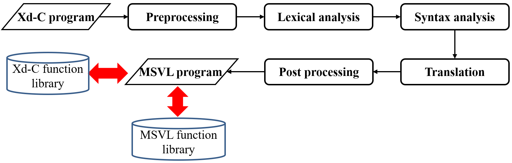
Refer to caption
Figure 3: Architecture of C​2​MC2M

In order to show the usability and scalability of our tool in translating real-world Xd-C programs to MSVL programs, we have applied C​2​MC2M on 13 programs from industry whose sizes range from ≈\approx 0.5k to ≈\approx 17k lines as shown in Table 7. In this benchmark, Xd-C programs from RERS P14 to RERS P19 are taken from RERS Grey-Box Challenge 2012 (RERS) [34]. LTLNFBA [35] is a software for translating an LTL formula to a Büchi automaton. Program carc [36] is a license plate recognition system. The other 5 programs bzip2, mcf, art, gzip and twolf are from SPEC2000 [29]. The experiments have been carried out on a 64-bit Windows 7 PC with a 4.00GHz Intel(R) Core(TM) i7 processor and 64GB memory.

Table 7 shows the experimental results on the benchmark. Column “Program” represents names of programs. Column “LOC” shows sizes of Xd-C programs and column “LOM” lists sizes of MSVL programs translated from Xd-C programs. Column “Time” shows the time consumed for accomplishing the translation tasks. Experimental results in Table 7 show that for all the programs, our tool can effectively output the translation results and the size of the generated MSVL programs is about 2.6 times of Xd-C Programs.

Table 7: Results of C2M on real-world programs
Program LOC LOM Time(s)
RERS P14 514 2261 0.46
RERS P15 1353 5016 2.04
RERS P16 1304 5271 2.18
RERS P17 2100 7753 4.38
RERS P18 3306 12677 11.81
RERS P19 8079 28332 63.83
LTLNFBA 3296 9113 0.76
carc 2170 4027 0.59
bzip2 2320 4976 0.55
mcf 1322 2124 0.36
art 886 1514 0.28
gzip 3773 8189 0.80
twolf 17452 33114 7.11
Total 47875 124376 95.15

7 Conclusion

In order to verify safety, reliability and security properties of C programs by means of a runtime verification tool UMC4M [18, 19] based on MSVL and its compiler MC [23], we need to translate C programs to MSVL programs automatically. In this paper, we first present an approach to translating programs written in Xd-C to MSVL programs. Then we prove the equivalence between an original Xd-C program and the translated MSVL program. For doing so, we inductively prove the equivalences between expressions and statements, respectively involved in the Xd-C and MSVL programs. Further, we have developed a translator C​2​MC2M based on the proposed algorithms. Moreover, to evaluate usability and scalability of C​2​MC2M, a benchmark of experiments including 13 programs from industry has been conducted. The results show that C​2​MC2M works effectively. However, since Xd-C is only a fragment of ANSI-C, to translate a general C program to an MSVL program, we have to manually translate the C program to an Xd-C program first.

In the near future, we plan to further optimize the translating approach and tool so as to improve efficiency of transformation. Further, we will build a library of functions for MSVL so that a large scale MSVL program can effectively be built. In addition, to verify properties of safety, reliability and security of C programs more effectively, we will further investigate techniques of runtime verification at code level by using translator C​2​MC2M, MSVL compiler MC and verifier UMC4M of the toolkit MSV [37] such that C or MSVL programs in large scale can effectively be verified.

References

References

  • [1] E. M. Clarke, O. Grumberg, D. E. Long, Model checking and abstraction, ACM transactions on Programming Languages and Systems (TOPLAS) 16 (5) (1994) 1512–1542.
  • [2] E. M. Clarke, O. Grumberg, D. Peled, Model checking, MIT press, 1999.
  • [3] A. Cimatti, E. Clarke, E. Giunchiglia, F. Giunchiglia, M. Pistore, M. Roveri, R. Sebastiani, A. Tacchella, NuSMV 2: An opensource tool for symbolic model checking, in: Proceedings of the 14th International Conference on Computer Aided Verification (CAV), Vol. 2404 of Lecture Notes in Computer Science, Springer, 2002, pp. 359–364.
  • [4] G. J. Holzmann, The model checker SPIN, IEEE Transactions on Software Engineering 23 (5) (1997) 279–295.
  • [5] A. Pnueli, The temporal logic of programs, in: Proceedings of the 18th Annual Symposium on Foundations of Computer Science (FOCS), IEEE Computer Society, 1977, pp. 46–57.
  • [6] E. M. Clarke, E. A. Emerson, A. P. Sistla, Automatic verification of finite-state concurrent systems using temporal logic specifications, ACM Transactions on Programming Languages and Systems (TOPLAS) 8 (2) (1986) 244–263.
  • [7] M. Gheorghe, R. Ceterchi, F. Ipate, S. Konur, R. Lefticaru, Kernel p systems: From modelling to verification and testing, Theoretical Computer Science 724 (2018) 45 – 60.
  • [8] A. Natarajan, H. Chauhan, N. Mittal, V. K. Garg, Efficient abstraction algorithms for predicate detection, Theoretical Computer Science 688 (2017) 24 – 48.
  • [9] F. Ivancic, I. Shlyakhter, A. Gupta, M. K. Ganai, V. Kahlon, C. Wang, Z. Yang, Model checking C programs using F-SOFT, in: Proceedings of 23rd International Conference on Computer Design (ICCD), IEEE Computer Society, 2005, pp. 297–308.
  • [10] T. A. Henzinger, R. Jhala, R. Majumdar, G. Sutre, Lazy abstraction, in: Proceedings of the 29th ACM SIGPLAN-SIGACT Symposium on Principles of Programming Languages (POPL), ACM, 2002, pp. 58–70.
  • [11] D. Beyer, A. Cimatti, A. Griggio, M. E. Keremoglu, R. Sebastiani, Software model checking via large-block encoding, in: Proceedings of 9th International Conference on Formal Methods in Computer-Aided Design (FMCAD), IEEE, 2009, pp. 25–32.
  • [12] D. Dietsch, M. Heizmann, V. Langenfeld, A. Podelski, Fairness modulo theory: A new approach to LTL software model checking, in: Proceedings of the 27th International Conference on Computer Aided Verification (CAV), Vol. 9206 of Lecture Notes in Computer Science, Springer, 2015, pp. 49–66.
  • [13] T. Ball, S. K. Rajamani, Automatically validating temporal safety properties of interfaces, in: Proceedings of the 8th international SPIN workshop on Model checking of software, Vol. 2057 of Lecture Notes in Computer Science, Springer, 2001, pp. 103–122.
  • [14] D. Beyer, T. A. Henzinger, R. Jhala, R. Majumdar, The software model checker BLAST: Applications to software engineering, International Journal on Software Tools for Technology Transfer 9 (5) (2007) 505–525.
  • [15] D. Beyer, M. E. Keremoglu, CPAchecker: A tool for configurable software verification, in: Proceedings of 23rd International Conference on Computer Aided Verification (CAV), Vol. 6806 of Lecture Notes in Computer Science, Springer, 2011, pp. 184–190.
  • [16] D. Kroening, M. Tautschnig, CBMC - C bounded model checker, in: Proceedings of 20th International Conference on Tools and Algorithms for the Construction and Analysis of Systems (TACAS), Vol. 8413 of Lecture Notes in Computer Science, Springer, 2014, pp. 389–391.
  • [17] M. Brockschmidt, B. Cook, S. Ishtiaq, H. Khlaaf, N. Piterman, T2: temporal property verification, in: Proceedings of the 22nd International Conference on Tools and Algorithms for the Construction and Analysis of Systems (TACAS), Vol. 9636 of Lecture Notes in Computer Science, Springer, 2016, pp. 387–393.
  • [18] M. Wang, C. Tian, Z. Duan, Full regular temporal property verification as dynamic program execution, in: Proceedings of the 39th International Conference on Software Engineering (ICSE) - Companion Volume, IEEE Computer Society, 2017, pp. 226–228.
  • [19] M. Wang, C. Tian, N. Zhang, Z. Duan, Verifying full regular temporal properties of programs via dynamic program execution, IEEE Transactions on Reliability (2018) 1–16doi:10.1109/TR.2018.2876333.
  • [20] Z. Duan, An extended interval temporal logic and a framing technique for temporal logic programming, Ph.D. thesis, Department of Computer Science, Newcastle University, Newcastle upon Tyne, UK (1996).
  • [21] Z. Duan, Temporal logic and temporal logic programming, Alexandria, NSW, Australia: Science Press, 2005.
  • [22] N. Zhang, Z. Duan, C. Tian, A mechanism of function calls in MSVL, Theoretical Computer Science 654 (2016) 11–25.
  • [23] K. Yang, Z. Duan, C. Tian, N. Zhang, A compiler for MSVL and its applications, Theoretical Computer Science 749 (2018) 2–16.
  • [24] Z. Duan, C. Tian, A practical decision procedure for propositional projection temporal logic with infinite models, Theoretical Computer Science 554 (2014) 169–190.
  • [25] Z. Duan, C. Tian, L. Zhang, A decision procedure for propositional projection temporal logic with infinite models, Acta Informatica 45 (1) (2008) 43–78.
  • [26] S. Blazy, X. Leroy, Mechanized semantics for the Clight subset of the C language, Journal of Automated Reasoning 43 (3) (2009) 263–288.
  • [27] X. Yang, Z. Duan, Operational semantics of framed tempura, The Journal of Logic and Algebraic Programming 78 (1) (2008) 22–51.
  • [28] X. Wang, C. Tian, Z. Duan, L. Zhao, MSVL: a typed language for temporal logic programming, Frontiers of Computer Science 11 (5) (2017) 762–785.
  • [29] Standard Performance Evaluation Corporation. SPEC CINT2000, October 2008., http://www.spec.org/cpu/CINT2000/.
  • [30] Z. Duan, X. Yang, M. Koutny, Framed temporal logic programming, Science of Computer Programming 70 (1) (2008) 31–61.
  • [31] Z. Duan, M. Koutny, A framed temporal logic programming language, Journal of Computer Science and Technology 19 (3) (2004) 341–351.
  • [32] S. Blazy, Z. Dargaye, X. Leroy, Formal verification of a C compiler front-end, in: Proceedings of the 14th International Symposium on Formal Methods (FM), Vol. 4085 of Lecture Notes in Computer Science, Springer, 2006, pp. 460–475.
  • [33] http://www.mingw.org/ (2018).
  • [34] F. Howar, M. Isberner, M. Merten, B. Steffen, D. Beyer, The RERS grey-box challenge 2012: Analysis of event-condition-action systems, in: Proceedings of the 5th International Symposium on Leveraging Applications of Formal Methods, Verification and Validation (ISoLA), Vol. 7609 of Lecture Notes in Computer Science, Springer, 2012, pp. 608–614.
  • [35] http://web.xidian.edu.cn/ctian/en/ltlnfba.html (2018).
  • [36] http://www.codeforge.cn/read/234151/car.c__html (2014).
  • [37] N. Zhang, Z. Duan, C. Tian, Model checking concurrent systems with MSVL, SCIENCE CHINA Information Sciences 59 (11) (2016) 118101.

Appendix

Appendix A: Operational Semantics of Xd-C

The following is operational semantics of expressions in Xd-C.

Expressions in left-value position:

E⁡(i​d)=b​o​r​(i​d∉D​o​m​(E)​a​n​d​s​y​m​b​o​l​(G,i​d)=⌊b⌋)G,E⊢i​d,M⇒l(b,0)​(C​1)G,E⊢e,M⇒p​t​r​(ℓ)G,E⊢∗e,M⇒lℓ​(C​2)G,E⊢l​e,M⇒l(b,δ)​t​y​p​e​(l​e)=s​t​r​u​c​t​i​d′​{φ}​𝑓𝑖𝑒𝑙𝑑​_​𝑜𝑓𝑓𝑠𝑒𝑡​(x,φ)=⌊δ′⌋G,E⊢l​e.x,M⇒l(b,δ+δ′)​(C​3)\begin{array}[]{l}\frac{E(id)=b~or~(id\notin Dom(E)~and~symbol(G,id)=\lfloor b\rfloor)}{G,E~\vdash~id,~M\stackrel{{\scriptstyle l}}{{\Rightarrow}}(b,0)}{\scriptstyle(C1)}~~~~~~~~\frac{G,E~\vdash~e,~M\Rightarrow ptr(\ell)}{G,E~\vdash~*e,M\stackrel{{\scriptstyle l}}{{\Rightarrow}}\ell}{\scriptstyle(C2)}\\ \frac{G,E~\vdash~le,~M\stackrel{{\scriptstyle l}}{{\Rightarrow}}(b,\delta)~~type(le)=struct~id^{\prime}\{\varphi\}~~\mathit{field\_offset}(x,\varphi)=\lfloor\delta^{\prime}\rfloor}{G,E~\vdash~le.x,~M\stackrel{{\scriptstyle l}}{{\Rightarrow}}(b,\delta+\delta^{\prime})}{\scriptstyle(C3)}\end{array}

where D​o​m​(E)Dom(E) is the domain of EE; p​t​r​(ℓ)ptr(\ell) is a pointer value pointing to ℓ\ell; t​y​p​e​(e)type(e) returns the type of ee; s​t​r​u​c​t​i​d′​{φ}struct~id^{\prime}\{\varphi\} is a struct type where i​d′id^{\prime} is the name and a list φ\varphi is its fields; 𝑓𝑖𝑒𝑙𝑑​_​𝑜𝑓𝑓𝑠𝑒𝑡​(x,φ)\mathit{field\_offset}(x,\varphi) returns the byte offset of the field named xx in a struct whose field list is φ\varphi.

In order to access and store values in memory locations, l​o​a​d​v​a​l​(τ,M,(b,δ))loadval(\tau,M,(b,\delta)) and s​t​o​r​e​v​a​l​(τ,M,(b,δ),v)storeval(\tau,M,(b,\delta),v) are respectively defined as follows:

Access modes:μ::=B​y​_​v​a​l​u​e​(κ)access by value∣By_referenceaccess by reference∣By_nothingno accessAssociating acess modes to Xd-C types:A⁡(s​i​g​n​e​d​c​h​a​r)=A⁡(c​h​a​r)=B​y​_​v​a​l​u​e​(i​n​t​8​s​i​g​n​e​d)A⁡(u​n​s​i​g​n​e​d​c​h​a​r)=B​y​_​v​a​l​u​e​(i​n​t​8​u​n​s​i​g​n​e​d)A⁡(s​i​g​n​e​d​s​h​o​r​t​i​n​t)=A⁡(s​h​o​r​t​i​n​t)=B​y​_​v​a​l​u​e​(i​n​t​16​s​i​g​n​e​d)A⁡(u​n​s​i​g​n​e​d​s​h​o​r​t​i​n​t)=B​y​_​v​a​l​u​e​(i​n​t​16​u​n​s​i​g​n​e​d)A⁡(s​i​g​n​e​d​i​n​t)=A⁡(u​n​s​i​g​n​e​d​i​n​t)=A⁡(i​n​t)=B​y​_​v​a​l​u​e​(i​n​t​32)A⁡(f​l​o​a​t)=B​y​_​v​a​l​u​e​(f​l​o​a​t​32)A⁡(d​o​u​b​l​e)=B​y​_​v​a​l​u​e​(f​l​o​a​t​64)A⁡(l​o​n​g​d​o​u​b​l​e)=B​y​_​v​a​l​u​e​(f​l​o​a​t​64)A(τ∗)=By_value(int32)A⁡(a​r​r​a​y)=B​y​_​r​e​f​e​r​e​n​c​eA⁡(s​t​r​u​c​t)=B​y​_​n​o​t​h​i​n​gA⁡(v​o​i​d)=B​y​_​n​o​t​h​i​n​gAccessing or updating a value of type τ at location (b,δ) in memory state M:l​o​a​d​v​a​l​(τ,M,(b,δ))=l​o​a​d​(κ,M,b,δ)if ​A​(τ)=B​y​_​v​a​l​u​e​(κ)l​o​a​d​v​a​l​(τ,M,(b,δ))=⌊p​t​r​(b,δ)⌋if ​A​(τ)=B​y​_​r​e​f​e​r​e​n​c​el​o​a​d​v​a​l​(τ,M,(b,δ))=∅if ​A​(τ)=B​y​_​n​o​t​h​i​n​gs​t​o​r​e​v​a​l​(τ,M,(b,δ),v)=s​t​o​r​e​(κ,M,b,δ,v)if ​A​(τ)=B​y​_​v​a​l​u​e​(κ)s​t​o​r​e​v​a​l​(τ,M,(b,δ),v)=∅otherwise\begin{array}[]{l}\begin{array}[]{llll}\mbox{Access modes:}&\mu&::=By\_value(\kappa)&\mbox{access by value}\\ &&~~\mid By\_reference&\mbox{access by reference}\\ &&~~\mid By\_nothing&\mbox{no access}\end{array}\\ \begin{array}[]{l}\mbox{Associating acess modes to Xd-C types:}\\ \begin{array}[]{l}A(signed~char)=A(char)=By\_value(int8signed)\\ A(unsigned~char)=By\_value(int8unsigned)\\ A(signed~short~int)=A(short~int)=By\_value(int16signed)\\ A(unsigned~short~int)=By\_value(int16unsigned)\\ A(signed~int)=A(unsigned~int)=A(int)=By\_value(int32)\\ A(float)=By\_value(float32)\\ A(double)=By\_value(float64)\\ A(long~double)=By\_value(float64)\\ A(\tau*)=By\_value(int32)\\ A(array)=By\_reference\\ A(struct)=By\_nothing\\ A(void)=By\_nothing\end{array}\\ \mbox{Accessing or updating a value of type $\tau$ at location $(b,\delta)$ in memory state $M$:}\\ \begin{array}[]{rll}loadval(\tau,M,(b,\delta))&=load(\kappa,M,b,\delta)&\mbox{if }A(\tau)=By\_value(\kappa)\\ loadval(\tau,M,(b,\delta))&=\lfloor ptr(b,\delta)\rfloor&\mbox{if }A(\tau)=By\_reference\\ loadval(\tau,M,(b,\delta))&=\emptyset&\mbox{if }A(\tau)=By\_nothing\\ storeval(\tau,M,(b,\delta),v)&=store(\kappa,M,b,\delta,v)&\mbox{if }A(\tau)=By\_value(\kappa)\\ storeval(\tau,M,(b,\delta),v)&=\emptyset&\mbox{otherwise}\end{array}\end{array}\end{array}

l​o​a​d​v​a​l​(τ,M,(b,δ))loadval(\tau,M,(b,\delta)) reads consecutive bytes at (b,δ)(b,\delta) in memory state MM and returns the contents of these bytes as value vv if successful while s​t​o​r​e​v​a​l​(τ,M,(b,δ),v)storeval(\tau,M,(b,\delta),\linebreak v) stores value vv at (b,δ)(b,\delta) in memory state MM and returns an updated memory state.

Expressions in right-value position:

G,E⊢c,M⇒c⁡(C​4)G,E⊢l​e,M⇒lℓ​l​o​a​d​v​a​l​(t​y​p​e​(l​e),M,ℓ)=⌊v⌋G,E⊢l​e,M⇒v​(C​5)G,E⊢l​e,M⇒lℓG,E⊢&l​e,M⇒p​t​r​(ℓ)​(C​6)G,E⊢e1,M⇒v1​e​v​a​l​_​u​n​o​p​(o​p1,v1,t​y​p​e​(e1))=⌊v⌋G,E⊢o​p1​e1,M⇒v​(C​7)G,E⊢e1,M⇒v1​G,E⊢e2,M⇒v2​e​v​a​l​_​b​i​n​o​p​(o​p2,v1,t​y​p​e​(e1),v2,t​y​p​e​(e2))=⌊v⌋G,E⊢e1​o​p2​e2,M⇒v​(C​8)G,E⊢e1,M⇒v1​i​s​_​t​r​u​e​(v1,t​y​p​e​(e1))​G,E⊢e2,M⇒v2G,E⊢e1​?​e2:e3,M⇒v2(C9)G,E⊢e1,M⇒v1​i​s​_​f​a​l​s​e​(v1,t​y​p​e​(e1))​G,E⊢e3,M⇒v3G,E⊢e1​?​e2:e3,M⇒v3(C10)G,E⊢e,M⇒v1​c​a​s​t​(v1,t​y​p​e​(e),τ)=⌊v⌋G,E⊢(τ)​e,M⇒v​(C​11)G,E⊢ef​u​n​(ea​r​g​s),M⇒tv,MG,E⊢ef​u​n​(ea​r​g​s),M⇒v​(C​12)\begin{array}[]{l}{\scriptstyle G,E~\vdash~c,~M\Rightarrow c~~(C4)}~~~~~~~~~~~\frac{G,E~\vdash~le,~M\stackrel{{\scriptstyle l}}{{\Rightarrow}}\ell~~loadval(type(le),M,\ell)=\lfloor v\rfloor}{G,E~\vdash~le,~M\Rightarrow v}~~{\scriptstyle(C5)}\\ \frac{G,E~\vdash~le,~M\stackrel{{\scriptstyle l}}{{\Rightarrow}}\ell}{G,E~\vdash~\&le,~M\Rightarrow ptr(\ell)}{\scriptstyle(C6)}~~~~\frac{G,E~\vdash~e_{1},~M\Rightarrow v_{1}~~eval\_unop(op_{1},v_{1},type(e_{1}))=\lfloor v\rfloor}{G,E~\vdash~op_{1}~e_{1},~M\Rightarrow v}{\scriptstyle(C7)}\\[6.45831pt] \frac{G,E~\vdash~e_{1},~M\Rightarrow v_{1}~~G,E~\vdash~e_{2},~M\Rightarrow v_{2}~~eval\_binop(op_{2},v_{1},type(e_{1}),v_{2},type(e_{2}))=\lfloor v\rfloor}{G,E~\vdash~e_{1}~op_{2}~e_{2},~M\Rightarrow v}{\scriptstyle(C8)}\\[6.45831pt] \frac{G,E~\vdash~e_{1},~M\Rightarrow v_{1}~~is\_true(v_{1},type(e_{1}))~~G,E~\vdash~e_{2},~M\Rightarrow v_{2}}{G,E~\vdash~e_{1}?e_{2}:e_{3},~M\Rightarrow v_{2}}{\scriptstyle(C9)}\\[6.45831pt] \frac{G,E~\vdash~e_{1},~M\Rightarrow v_{1}~~is\_false(v_{1},type(e_{1}))~~G,E~\vdash~e_{3},~M\Rightarrow v_{3}}{G,E~\vdash~e_{1}?e_{2}:e_{3},~M\Rightarrow v_{3}}{\scriptstyle(C10)}\\[6.45831pt] \frac{G,E~\vdash~e,~M\Rightarrow v_{1}~~cast(v_{1},type(e),\tau)=\lfloor v\rfloor}{G,E~\vdash~(\tau)e,~M\Rightarrow v}{\scriptstyle(C11)}\\ \frac{G,E~\vdash~e_{fun}(e_{args}),~M\stackrel{{\scriptstyle t}}{{\Rightarrow}}v,~M}{G,E~\vdash~e_{fun}(e_{args}),~M{\Rightarrow}v}{\scriptstyle(C12)}\end{array}

where e​v​a​l​_​u​n​o​p​(o​p1,v1,t​y​p​e​(e1))eval\_unop(op_{1},v_{1},type(e_{1})) describes a unary operation and returns the value of o​p1​v1op_{1}~v_{1}; e​v​a​l​_​b​i​n​o​p​(o​p2,v1,t​y​p​e​(e1),v2,t​y​p​e​(e2))eval\_binop(op_{2},v_{1},type(e_{1}),v_{2},type(e_{2})) returns the value of v1​o​p2​v2v_{1}~op_{2}~v_{2}; i​s​_​t​r​u​e​(v1,t​y​p​e​(e1))is\_true(v_{1},type(e_{1})) and i​s​_​f​a​l​s​e​(v1,t​y​p​e​(e1))is\_false(v_{1},type(e_{1})) determine the truth value of v1v_{1}, depending on its type, and the truth value of v1v_{1} is false if v1v_{1} equals 0 and true otherwise; c​a​s​t​(v1,t​y​p​e​(e),τ)cast(v_{1},type(e),\tau) converts v1v_{1} from its natural type t​y​p​e​(e)type(e) to the expected type τ\tau.

Taking binary addition as an example, the two argument expressions of types τ1\tau_{1} and τ2\tau_{2} are evaluated and their values v1v_{1} and v2v_{2} are combined using the the e​v​a​l​_​b​i​n​o​peval\_binop function. The cases corresponding to binary addition are shown in Table 8.

Table 8: Binary addition
τ1\tau_{1} τ2\tau_{2} v1v_{1} v2v_{2} e​v​a​l​_​b​i​n​o​p​(+,v1,τ1,v2,τ2)eval\_binop(+,v_{1},\tau_{1},v_{2},\tau_{2})
i​n​tint i​n​tint n1n_{1} n2n_{2} n1+n2n_{1}+n_{2}
f​l​o​a​tfloat f​l​o​a​tfloat f1f_{1} f2f_{2} f1+f2f_{1}+f_{2}
d​o​u​b​l​edouble d​o​u​b​l​edouble d1d_{1} d2d_{2} d1+d2d_{1}+d_{2}
τ∗\tau* i​n​tint p​t​r​(b,δ)ptr(b,\delta) nn p​t​r​(b,δ+n∗s​i​z​e​o​f​(τ))ptr(b,\delta+n*sizeof(\tau))
i​n​tint τ∗\tau* nn p​t​r​(b,δ)ptr(b,\delta) p​t​r​(b,δ+n∗s​i​z​e​o​f​(τ))ptr(b,\delta+n*sizeof(\tau))
otherwise ∅\emptyset

Some forms of C expressions are omitted but can be expressed as syntactic sugar:

array access:id[e]≡∗(id+e)C13id[e1][e2]≡∗(id+e1∗n+e2),where n is the number of elements in each row of i​d​[e1]​[e2].​C​14indirect field access:e→x≡∗(e.x)C15\begin{array}[]{ll}\mbox{array access:}&id[e]\equiv*(id+e)~~~C13\\ &id[e_{1}][e_{2}]\equiv*(id+e_{1}*n+e_{2}),\mbox{where $n$ is the number }\\ &\mbox{of elements in each row of $id[e_{1}][e_{2}]$.}~~~C14\\ \mbox{indirect field access:}&e\rightarrow x\equiv*(e.x)~~~C15\\ \end{array}

Operational semantics for Xd-C statements (other than loops and switch statements):

G,E⊢;,M⇒ϵN​o​r​m​a​l,M⁡(T​1)G,E⊢break;,M⇒ϵB​r​e​a​k,M⁡(T​2)G,E⊢continue;,M⇒ϵC​o​n​t​i​n​u​e,M⁡(T​3)G,E⊢return;,M⇒ϵR​e​t​u​r​n,M⁡(T​4)G,E⊢e,M⇒v,M′G,E⊢return ​e;,M⇒ϵR​e​t​u​r​n​(v),M′(T​5)G,E⊢l​e,M⇒lℓG,E⊢e,M⇒vs​t​o​r​e​v​a​l​(t​y​p​e​(l​e),M,ℓ,v)=⌊M′⌋G,E⊢l​e=e,M⇒ϵN​o​r​m​a​l,M′​(T​6)G,E⊢c​s1,M⇒t1N​o​r​m​a​l,M1​G,E⊢c​s2,M1⇒t2o​u​t,M2G,E⊢(c​s1;c​s2),M⇒t1.t2o​u​t,M2​(T​7)G,E⊢c​s1,M⇒to​u​t,M′​o​u​t≠N​o​r​m​a​lG,E⊢(c​s1;c​s2),M⇒to​u​t,M′​(T​8)G,E⊢e,M⇒v​i​s​_​t​r​u​e​(v,t​y​p​e​(e))​G,E⊢c​s1,M⇒to​u​t,M′G,E⊢if(e)​{c​s1}else{c​s2},M⇒to​u​t,M′​(T​9)G,E⊢e,M⇒v​i​s​_​f​a​l​s​e​(v,t​y​p​e​(e))​G,E⊢c​s2,M⇒to​u​t,M′G,E⊢if(e)​{c​s1}else{c​s2},M⇒to​u​t,M′​(T​10)\begin{array}[]{c}{\scriptstyle G,E~\vdash~;,~M\stackrel{{\scriptstyle\epsilon}}{{\Rightarrow}}Normal,~M~~(T1)}~~~~~~~~~~~{\scriptstyle G,E~\vdash~\mbox{{\scriptsize break}};,~M\stackrel{{\scriptstyle\epsilon}}{{\Rightarrow}}Break,~M~~(T2)}\\ {\scriptstyle G,E~\vdash~\mbox{{\scriptsize continue}};,~M\stackrel{{\scriptstyle\epsilon}}{{\Rightarrow}}Continue,~M~~(T3)~~~~~~~~~~~G,E~\vdash~\mbox{{\scriptsize return}};,~M\stackrel{{\scriptstyle\epsilon}}{{\Rightarrow}}Return,~M~~(T4)}\\[4.30554pt] \frac{G,E~\vdash~e,~M\Rightarrow v,~M^{\prime}}{G,E~\vdash~\mbox{{\scriptsize return }}e;,~M\stackrel{{\scriptstyle\epsilon}}{{\Rightarrow}}Return(v),M^{\prime}}~~~~{\scriptstyle(T5)}\\[6.45831pt] \frac{G,E~\vdash~le,~M\stackrel{{\scriptstyle l}}{{\Rightarrow}}\ell~~~~G,E~\vdash~e,~M\Rightarrow v~~~~storeval(type(le),M,\ell,v)=\lfloor M^{\prime}\rfloor}{G,E~\vdash~le=e,~M\stackrel{{\scriptstyle\epsilon}}{{\Rightarrow}}Normal,~M^{\prime}}{\scriptstyle(T6)}\\[6.45831pt] \frac{G,E~\vdash~cs_{1},~M\stackrel{{\scriptstyle t_{1}}}{{\Rightarrow}}Normal,~M_{1}~~G,E~\vdash~cs_{2},~M_{1}\stackrel{{\scriptstyle t_{2}}}{{\Rightarrow}}out,~M_{2}}{G,E~\vdash~(cs_{1};cs_{2}),~M\stackrel{{\scriptstyle t_{1}.t_{2}}}{{\Rightarrow}}out,M_{2}}{\scriptstyle(T7)}\\[6.45831pt] \frac{G,E~\vdash~cs_{1},~M\stackrel{{\scriptstyle t}}{{\Rightarrow}}out,~M^{\prime}~~out\neq Normal}{G,E~\vdash~(cs_{1};cs_{2}),~M\stackrel{{\scriptstyle t}}{{\Rightarrow}}out,M^{\prime}}{\scriptstyle(T8)}\\[6.45831pt] \frac{G,E~\vdash~e,~M\Rightarrow v~~~is\_true(v,type(e))~~~G,E~\vdash~cs_{1},~M\stackrel{{\scriptstyle t}}{{\Rightarrow}}out,~M^{\prime}}{G,E~\vdash~\mbox{{\scriptsize if$(e)\{cs_{1}\}$else$\{cs_{2}\}$}},~M\stackrel{{\scriptstyle t}}{{\Rightarrow}}out,~M^{\prime}}~~{\scriptstyle(T9)}\\[6.45831pt] \frac{G,E~\vdash~e,~M\Rightarrow v~~~is\_false(v,type(e))~~~G,E~\vdash~cs_{2},~M\stackrel{{\scriptstyle t}}{{\Rightarrow}}out,~M^{\prime}}{G,E~\vdash~\mbox{{\scriptsize if$(e)\{cs_{1}\}$else$\{cs_{2}\}$}},~M\stackrel{{\scriptstyle t}}{{\Rightarrow}}out,~M^{\prime}}~~{\scriptstyle(T10)}\end{array}

l​e++le\mathit{++} and l​e−−le\mathit{--} are omitted but can be expressed as follows:

l​e++≡(l​e=l​e+1)l​e−−≡(l​e=l​e−1)\begin{array}[]{ll}le\mathit{++}\equiv(le=le+1)\\ le\mathit{--}\equiv(le=le-1)\end{array}

The following rules define the execution of while and for loops. The rules describing the execution of do loops resemble the rules for while loops and are omitted in this paper.
Outcome updates (at the end of a loop execution):

B​r​e​a​k↝l​o​o​pN​o​r​m​a​l​R​e​t​u​r​n↝l​o​o​pR​e​t​u​r​n​R​e​t​u​r​n​(v)↝l​o​o​pR​e​t​u​r​n​(v){\scriptstyle Break~\stackrel{{\scriptstyle loop}}{{\rightsquigarrow}}~Normal~~~Return\stackrel{{\scriptstyle loop}}{{\rightsquigarrow}}Return~~~Return(v)\stackrel{{\scriptstyle loop}}{{\rightsquigarrow}}Return(v)}

while loops:

G,E⊢e,M⇒v​i​s​_​f​a​l​s​e​(v,t​y​p​e​(e))G,E⊢while​(e)​{c​s},M⇒ϵN​o​r​m​a​l,M​(T​11)G,E⊢e,M⇒v​i​s​_​t​r​u​e​(v,t​y​p​e​(e))​G,E⊢c​s,M⇒to​u​t,M′​o​u​t↝l​o​o​po​u​t′G,E⊢while​(e)​{c​s},M⇒to​u​t′,M′​(T​12)G,E⊢e,M⇒v​i​s​_​t​r​u​e​(v,t​y​p​e​(e))G,E⊢c​s,M⇒t1(N​o​r​m​a​l|C​o​n​t​i​n​u​e),M1​G,E⊢while​(e)​{c​s},M1⇒t2o​u​t′,M2G,E⊢while​(e)​{c​s},M⇒t1.t2o​u​t′,M2​(T​13)\begin{array}[]{c}\frac{G,E~\vdash~e,~M\Rightarrow v~~~is\_false(v,type(e))}{G,E~\vdash~\mbox{{\scriptsize while}}(e)\{cs\},~M\stackrel{{\scriptstyle\epsilon}}{{\Rightarrow}}Normal,~M}~~{\scriptstyle(T11)}\\[4.30554pt] \frac{G,E~\vdash~e,~M\Rightarrow v~~~is\_true(v,type(e))~~~G,E~\vdash~cs,~M\stackrel{{\scriptstyle t}}{{\Rightarrow}}out,~M^{\prime}~~~out\stackrel{{\scriptstyle loop}}{{\rightsquigarrow}}out^{\prime}}{G,E~\vdash~\mbox{{\scriptsize while}}(e)\{cs\},~M\stackrel{{\scriptstyle t}}{{\Rightarrow}}out^{\prime},~M^{\prime}}~~{\scriptstyle(T12)}\\[8.61108pt] \frac{\begin{array}[]{c}\scriptstyle G,E~\vdash~e,~M\Rightarrow v~~~is\_true(v,type(e))\\ \scriptstyle G,E~\vdash~cs,~M\stackrel{{\scriptstyle t_{1}}}{{\Rightarrow}}(Normal|Continue),~M_{1}~~~G,E~\vdash~\mbox{{\scriptsize while}}(e)\{cs\},~M_{1}\stackrel{{\scriptstyle t_{2}}}{{\Rightarrow}}out^{\prime},M_{2}\end{array}}{G,E~\vdash~\mbox{{\scriptsize while}}(e)\{cs\},~M\stackrel{{\scriptstyle t_{1}.t_{2}}}{{\Rightarrow}}out^{\prime},M_{2}}~~{\scriptstyle(T13)}\end{array}

for loops:

cs1≠;G,E⊢cs1,M⇒t1Normal,M1G,E⊢for(;e;cs2){cs},M1⇒t2out,M2G,E⊢for​(c​s1,e,c​s2)​{c​s},M⇒t1.t2o​u​t,M2​(T​14)G,E⊢e,M⇒v​i​s​_​f​a​l​s​e​(v,t​y​p​e​(e))G,E⊢for(;e;cs2){cs},M⇒ϵNormal,M​(T​15)G,E⊢e,M⇒v​i​s​_​t​r​u​e​(v,t​y​p​e​(e))​G,E⊢c​s,M⇒to​u​t1,M′​o​u​t1↝l​o​o​po​u​tG,E⊢for(;e;cs2){cs},M⇒tout,M′​(T​16)G,E⊢e,M⇒v​i​s​_​t​r​u​e​(v,t​y​p​e​(e))​G,E⊢c​s,M⇒t1(N​o​r​m​a​l|C​o​n​t​i​n​u​e),M1G,E⊢cs2,M1⇒t2Normal,M2G,E⊢for(;e;cs2){cs},M2⇒t3out,M3G,E⊢for(;e;cs2){cs},M⟹t1.t2.t3out,M3​(T​17)\begin{array}[]{c}\frac{cs_{1}\neq;~~~\scriptstyle G,E~\vdash~cs_{1},~M\stackrel{{\scriptstyle t_{1}}}{{\Rightarrow}}Normal,~M_{1}~~~G,E~\vdash~\mbox{\scriptsize for}(;e;cs_{2})\{cs\},~M_{1}\stackrel{{\scriptstyle t_{2}}}{{\Rightarrow}}out,~M_{2}}{G,E~\vdash~\mbox{\scriptsize for}(cs_{1};e;cs_{2})\{cs\},~M\stackrel{{\scriptstyle t_{1}.t_{2}}}{{\Rightarrow}}out,~M_{2}}~~{\scriptstyle(T14)}\\[8.61108pt] \frac{G,E~\vdash~e,~M\Rightarrow v~~~is\_false(v,type(e))}{G,E~\vdash~\mbox{\scriptsize for}(;e;cs_{2})\{cs\},~M\stackrel{{\scriptstyle\epsilon}}{{\Rightarrow}}Normal,~M}~~{\scriptstyle(T15)}\\[8.61108pt] \frac{\begin{array}[]{c}\scriptstyle G,E~\vdash~e,~M\Rightarrow v~~~is\_true(v,type(e))~~~\scriptstyle G,E~\vdash~cs,~M\stackrel{{\scriptstyle t}}{{\Rightarrow}}out_{1},~M^{\prime}~~~out_{1}\stackrel{{\scriptstyle loop}}{{\rightsquigarrow}}out\end{array}}{G,E~\vdash~\mbox{\scriptsize for}(;e;cs_{2})\{cs\},~M\stackrel{{\scriptstyle t}}{{\Rightarrow}}out,~M^{\prime}}~~{\scriptstyle(T16)}\\[8.61108pt] \frac{\begin{array}[]{c}\scriptstyle G,E~\vdash~e,~M\Rightarrow v~~~is\_true(v,type(e))~~~G,E~\vdash~cs,~M\stackrel{{\scriptstyle t_{1}}}{{\Rightarrow}}(Normal|Continue),~M_{1}\\ \scriptstyle G,E~\vdash~cs_{2},~M_{1}\stackrel{{\scriptstyle t_{2}}}{{\Rightarrow}}Normal,~M_{2}~~~G,E~\vdash~\mbox{\scriptsize for}(;e;cs_{2})\{cs\},~M_{2}\stackrel{{\scriptstyle t_{3}}}{{\Rightarrow}}out,~M_{3}\end{array}}{G,E~\vdash~\mbox{\scriptsize for}(;e;cs_{2})\{cs\},~M\stackrel{{\scriptstyle t_{1}.t_{2}.t_{3}}}{{\Longrightarrow}}out,~M_{3}}~~{\scriptstyle(T17)}\end{array}

Outcome updates (at the end of a switch execution):

N​o​r​m​a​l↝s​w​i​t​c​hN​o​r​m​a​l​C​o​n​t​i​n​u​e↝s​w​i​t​c​hC​o​n​t​i​n​u​e​B​r​e​a​k↝s​w​i​t​c​hN​o​r​m​a​lR​e​t​u​r​n↝s​w​i​t​c​hR​e​t​u​r​nR​e​t​u​r​n​(v)↝s​w​i​t​c​hR​e​t​u​r​n​(v){\begin{array}[]{l}\scriptstyle Normal~\stackrel{{\scriptstyle switch}}{{\rightsquigarrow}}~Normal~~~Continue~\stackrel{{\scriptstyle switch}}{{\rightsquigarrow}}~Continue~~~Break~\stackrel{{\scriptstyle switch}}{{\rightsquigarrow}}~Normal\\ \scriptstyle Return\stackrel{{\scriptstyle switch}}{{\rightsquigarrow}}Return~~~~~~Return(v)\stackrel{{\scriptstyle switch}}{{\rightsquigarrow}}Return(v)\end{array}}

switch(e)(e){case n0:c​s0;…;n_{0}:cs_{0};...;case nm:c​sm;n_{m}:cs_{m};default:c​s;:cs;}:

G,E⊢c​s,M⇒to​u​t,M′G,E⊢default:cs;,M⇒tout,M′(T18)G,E⊢c​s,M⇒to​u​t,M′G,E⊢case:cs;,M⇒tout,M′(T19)G,E⊢case ​ni:c​si;,M⇒t1N​o​r​m​a​l,M1G,E⊢case ni+1:c​si+1;…;case nm:c​sm;defalut:c​s;,M⇒t2out,M2G,E⊢case ni:c​si;…;case nm:c​sm;defalut:c​s;,M⇒t1.t2out,M2(T20)G,E⊢case ​ni:c​si;,M⇒to​u​t,M′​o​u​t≠N​o​r​m​a​lG,E⊢case ni:c​si;…;case nm:c​sm;defalut:c​s;,M⇒tout,M′(T21)G,E⊢e,M⇒v​v==niG,E⊢case ni:c​si;…;case nm:c​sm;defalut:c​s;,M⇒tout1,M′out1↝s​w​i​t​c​houtG,E⊢switch(e){case n0:c​s0;…;case nm:c​sm;defalut:c​s;},M⇒tout,M′(T22)G,E⊢e,M⇒v​v!=n0​v!=n1​…​v!=nmG,E⊢defalut:c​s;,M⇒tout1,M′out1↝s​w​i​t​c​houtG,E⊢switch(e){case n0:c​s0;…;case nm:c​sm;defalut:c​s;},M⇒tout,M′(T23)\begin{array}[]{c}\frac{G,E~\vdash~cs,~M\stackrel{{\scriptstyle t}}{{\Rightarrow}}out,~M^{\prime}}{G,E~\vdash~\mbox{{\scriptsize default:}}cs;,~M\stackrel{{\scriptstyle t}}{{\Rightarrow}}out,M^{\prime}}~~~~{\scriptstyle(T18)}~~~~~~~~~~~~~\frac{G,E~\vdash~cs,~M\stackrel{{\scriptstyle t}}{{\Rightarrow}}out,~M^{\prime}}{G,E~\vdash~\mbox{{\scriptsize case:}}cs;,~M\stackrel{{\scriptstyle t}}{{\Rightarrow}}out,M^{\prime}}~~~~{\scriptstyle(T19)}\\[6.45831pt] \frac{\begin{array}[]{c}\scriptstyle G,E~\vdash~\mbox{\scriptsize case }n_{i}:cs_{i};,~M\stackrel{{\scriptstyle t_{1}}}{{\Rightarrow}}Normal,~M_{1}\\ \scriptstyle G,E~\vdash~\mbox{\scriptsize case $n_{i+1}:cs_{i+1};...;$case $n_{m}:cs_{m};$defalut$:cs;$},~M\stackrel{{\scriptstyle t_{2}}}{{\Rightarrow}}out,~M_{2}\end{array}}{G,E~\vdash~\mbox{\scriptsize case $n_{i}:cs_{i};...;$case $n_{m}:cs_{m};$defalut$:cs;$},~M\stackrel{{\scriptstyle t_{1}.t_{2}}}{{\Rightarrow}}out,M_{2}}{\scriptstyle(T20)}\\[6.45831pt] \frac{G,E~\vdash~\mbox{\scriptsize case }n_{i}:cs_{i};,~M\stackrel{{\scriptstyle t}}{{\Rightarrow}}out,~M^{\prime}~~out\neq Normal}{G,E~\vdash~\mbox{\scriptsize case $n_{i}:cs_{i};...;$case $n_{m}:cs_{m};$defalut$:cs;$},~M\stackrel{{\scriptstyle t}}{{\Rightarrow}}out,M^{\prime}}{\scriptstyle(T21)}\\[6.45831pt] \frac{\begin{array}[]{c}\scriptstyle G,E~\vdash~e,~M\Rightarrow v~~~v==n_{i}\\ \scriptstyle G,E~\vdash~\mbox{\scriptsize case $n_{i}:cs_{i};...;$case $n_{m}:cs_{m};$defalut$:cs;$},~M\stackrel{{\scriptstyle t}}{{\Rightarrow}}out_{1},M^{\prime}~~~out_{1}\stackrel{{\scriptstyle switch}}{{\rightsquigarrow}}out\end{array}}{G,E~\vdash~\mbox{\scriptsize switch($e$)\lx@text@lbrace case $n_{0}:cs_{0};...;$case $n_{m}:cs_{m};$defalut$:cs;$\lx@text@rbrace},~M\stackrel{{\scriptstyle t}}{{\Rightarrow}}out,M^{\prime}}{\scriptstyle(T22)}\\[6.45831pt] \frac{\begin{array}[]{c}\scriptstyle G,E~\vdash~e,~M\Rightarrow v~~~v!=n_{0}~~~v!=n_{1}~~~...~~~v!=n_{m}\\ \scriptstyle G,E~\vdash~\mbox{\scriptsize defalut$:cs;$},~M\stackrel{{\scriptstyle t}}{{\Rightarrow}}out_{1},M^{\prime}~~~out_{1}\stackrel{{\scriptstyle switch}}{{\rightsquigarrow}}out\end{array}}{G,E~\vdash~\mbox{\scriptsize switch($e$)\lx@text@lbrace case $n_{0}:cs_{0};...;$case $n_{m}:cs_{m};$defalut$:cs;$\lx@text@rbrace},~M\stackrel{{\scriptstyle t}}{{\Rightarrow}}out,M^{\prime}}{\scriptstyle(T23)}\\[6.45831pt] \end{array}

Function calls:

G,E⊢ef​u​n,M⇒p​t​r​(b,0)​G,E⊢ea​r​g​s,M⇒va​r​g​s𝑓𝑢𝑛𝑐𝑡𝑑𝑒𝑓⁡(G,b)=⌊f​u​n​c​t⌋​t​y​p​e​_​o​f​_​f​u​n​d​e​f​(f​u​n​c​t)=t​y​p​e​(ef​u​n)G⊢funct(va​r​g​s),M⇒tvr​e​s,M′G,E⊢ef​u​n​(ea​r​g​s),M⇒tvr​e​s,M′​(T​24)\begin{array}[]{c}\frac{\begin{array}[]{c}\scriptstyle G,E~\vdash~e_{fun},~M\Rightarrow ptr(b,0)~~~G,E~\vdash~e_{args},~M\Rightarrow v_{args}\\ \scriptstyle\mathit{functdef}(G,b)=\lfloor funct\rfloor~~~type\_of\_fundef(funct)=type(e_{fun})\\ \scriptstyle G~\vdash~funct(v_{args}),~M\stackrel{{\scriptstyle t}}{{\Rightarrow}}v_{res},~M^{\prime}\end{array}}{G,E~\vdash~e_{fun}(e_{args}),~M\stackrel{{\scriptstyle t}}{{\Rightarrow}}v_{res},~M^{\prime}}~~{\scriptstyle(T24)}\end{array}

where ef​u​ne_{fun} is a function pointer or a function name, ea​r​g​se_{args} a list of arguments of the function and va​r​g​sv_{args} a list of values of arguments; t​y​p​e​_​o​f​_​f​u​n​d​e​f​(f​u​n​c​t)type\_of\_fundef(funct) returns the type of function f​u​n​c​tfunct including the return type and types of parameters; vr​e​sv_{res} is the return value of f​u​n​c​t​(va​r​g​s)funct(v_{args}).
Compatibility between values, outcomes and return types:

N​o​r​m​a​l,v​o​i​d​#​u​n​d​e​fR​e​t​u​r​n,v​o​i​d​#​u​n​d​e​fR​e​t​u​r​n​(v),τ​#​v​when ​τ≠v​o​i​d{\scriptstyle Normal,void\#undef~~~~Return,void\#undef~~~~Return(v),\tau\#v~\mbox{\scriptsize when }\tau\neq void}

Function invocations:

f​u​n​c​t=[τ∣v​o​i​d]​i​d​(p​a​r)​{d​c​l;c​s}​a​l​l​o​c​_​v​a​r​s​(M,p​a​r​+​d​c​l,E)=(M1,b∗)bind_params(E,M1,par,va​r​g​s)=M2G,E⊢cs,M2⇒tout,M3out,τ#vr​e​sG⊢funct(va​r​g​s),M⇒tvr​e​s,free(M3,b∗)​(T​25)f​u​n​c​t=e​x​t​e​r​n​[τ∣v​o​i​d]​i​d​(p​a​r)​vr​e​s=i​d​(va​r​g​s)​v=`​`​i​d​(va​r​g​s,vr​e​s)​"G⊢funct(va​r​g​s),M⇒vvr​e​s,M​(T​26)\begin{array}[]{c}\frac{\begin{array}[]{c}\scriptstyle funct=[\tau\mid void]~id(par)\{dcl;cs\}~~~alloc\_vars(M,par\textbf{+}dcl,E)=(M_{1},b^{*})\\ \scriptstyle bind\_params(E,M_{1},par,v_{args})=M_{2}~~~G,E~\vdash~cs,~M_{2}\stackrel{{\scriptstyle t}}{{\Rightarrow}}out,M_{3}~~~out,\tau\#v_{res}\end{array}}{G~\vdash funct(v_{args}),~M\stackrel{{\scriptstyle t}}{{\Rightarrow}}v_{res},~free(M_{3},b^{*})}~~{\scriptstyle(T25)}\\[8.61108pt] \frac{funct=extern~[\tau\mid void]~id(par)~~~v_{res}=id(v_{args})~~~v=``id(v_{args},v_{res})"}{G\vdash funct(v_{args}),~M\stackrel{{\scriptstyle v}}{{\Rightarrow}}v_{res},M}~~{\scriptstyle(T26)}\end{array}

where d​c​ldcl is a list of declarations (dcl=(Pd;)∗dcl=(Pd;)^{*}); a​l​l​o​c​_​v​a​r​s​(M,p​a​r​+​d​c​l,E)alloc\_vars(M,par\textbf{+}dcl,E) allocates the memory required for storing the formal parameters p​a​rpar and the local variables d​c​ldcl; b​i​n​d​_​p​a​r​a​m​s​(E,M1,p​a​r,va​r​g​s)bind\_params(E,M_{1},par,v_{args}) iterates the s​t​o​r​e​v​a​lstoreval function in order to initialize formal parameters p​a​rpar to the values of the corresponding arguments va​r​g​sv_{args}; vr​e​s=i​d​(va​r​g​s)v_{res}=id(v_{args}) obtains the return value of the function call i​d​(va​r​g​s)id(v_{args}) and if the return type is v​o​i​dvoid, the value of vv is ∅\emptyset. An input/output event vv recorded in the trace is generated by a call to an external function.
Operational semantics for divergence:

∀i∈N0(G,E⊢e,Mi⇒v∧is_true(v,type(e))∧G,E⊢cs,Mi⇒t(Normal∣Continue),Mi+1→G,E⊢e,Mi+1⇒v′∧is_true(v′,type(e)))∧M0=MG,E⊢while​(e)​{c​s},M⇒T∞​(D​1)G,E⊢c​s1,M⇒T∞G,E⊢c​s1;c​s2,M⇒T∞​(D​2)G,E⊢c​s1,M⇒tN​o​r​m​a​l,M1​G,E⊢c​s2,M1⇒T∞G,E⊢c​s1;c​s2,M⇒t.T∞​(D​3)G,E⊢e,M⇒v​i​s​_​t​r​u​e​(v,t​y​p​e​(e))​G,E⊢c​s1,M⇒T∞G,E⊢if(e)​{c​s1}else{c​s2},M⇒T∞​(D​4)G,E⊢e,M⇒v​i​s​_​f​a​l​s​e​(v,t​y​p​e​(e))​G,E⊢c​s2,M⇒T∞G,E⊢if(e)​{c​s1}else{c​s2},M⇒T∞​(D​5)G,E⊢e,M⇒v​i​s​_​t​r​u​e​(v,t​y​p​e​(e))​G,E⊢c​s,M⇒T∞G,E⊢while​(e)​{c​s},M⇒T∞​(D​6)G,E⊢e,M⇒v​i​s​_​t​r​u​e​(v,t​y​p​e​(e))G,E⊢c​s,M⇒t(N​o​r​m​a​l∣C​o​n​t​i​n​u​e),M1​G,E⊢while​(e)​{c​s},M1⇒T∞G,E⊢while​(e)​{c​s},M⇒t.T∞​(D​7)G,E⊢ef​u​n,M⇒p​t​r​(b,0)​G,E⊢ea​r​g​s,M⇒va​r​g​s𝑓𝑢𝑛𝑐𝑡𝑑𝑒𝑓⁡(G,b)=⌊f​u​n​c​t⌋​t​y​p​e​_​o​f​_​f​u​n​d​e​f​(f​u​n​c​t)=t​y​p​e​(ef​u​n)G⊢f​u​n​c​t​(va​r​g​s),M⇒T∞G,E⊢ef​u​n​(ea​r​g​s),M⇒T∞​(D​8)F=τ​i​d​(p​a​r)​{d​c​l;c​s}​a​l​l​o​c​_​v​a​r​s​(M,p​a​r​+​d​c​l,E)=(M1,b∗)b​i​n​d​_​p​a​r​a​m​s​(E,M1,p​a​r,va​r​g​s)=M2​G,E⊢c​s,M2⇒T∞G⊢F⁡(va​r​g​s),M⇒T∞​(D​9)\begin{array}[]{c}\frac{\begin{array}[]{c}\scriptstyle\forall i\in N_{0}(G,E~\vdash~e,~M_{i}{\Rightarrow}v\wedge is\_true(v,type(e))\wedge G,E~\vdash~cs,~M_{i}\stackrel{{\scriptstyle t}}{{\Rightarrow}}(Normal\mid Continue),~M_{i+1}\\ \scriptstyle\rightarrow G,E~\vdash~e,~M_{i+1}{\Rightarrow}v^{\prime}\wedge is\_true(v^{\prime},type(e)))\wedge M_{0}=M\end{array}}{G,E~\vdash~\mbox{\scriptsize while}(e)\{cs\},~M\stackrel{{\scriptstyle T}}{{\Rightarrow}}\infty}~{\scriptstyle(D1)}\\ \frac{G,E~\vdash~cs_{1},~M\stackrel{{\scriptstyle T}}{{\Rightarrow}}\infty}{G,E~\vdash~cs_{1};cs_{2},~M\stackrel{{\scriptstyle T}}{{\Rightarrow}}\infty}~{\scriptstyle(D2)}~~~~~\frac{G,E~\vdash~cs_{1},~M\stackrel{{\scriptstyle t}}{{\Rightarrow}}Normal,~M_{1}~~~G,E~\vdash~cs_{2},~M_{1}\stackrel{{\scriptstyle T}}{{\Rightarrow}}\infty}{G,E~\vdash~cs_{1};cs_{2},~M\stackrel{{\scriptstyle t.T}}{{\Rightarrow}}\infty}~{\scriptstyle(D3)}\\ \frac{G,E~\vdash~e,~M\Rightarrow v~~~is\_true(v,type(e))~~~G,E~\vdash~cs_{1},~M\stackrel{{\scriptstyle T}}{{\Rightarrow}}\infty}{G,E~\vdash~\mbox{{\scriptsize if$(e)\{cs_{1}\}$else$\{cs_{2}\}$}},~M\stackrel{{\scriptstyle T}}{{\Rightarrow}}\infty}~~{\scriptstyle(D4)}\\[6.45831pt] \frac{G,E~\vdash~e,~M\Rightarrow v~~~is\_false(v,type(e))~~~G,E~\vdash~cs_{2},~M\stackrel{{\scriptstyle T}}{{\Rightarrow}}\infty}{G,E~\vdash~\mbox{{\scriptsize if$(e)\{cs_{1}\}$else$\{cs_{2}\}$}},~M\stackrel{{\scriptstyle T}}{{\Rightarrow}}\infty}~~{\scriptstyle(D5)}\\ \frac{G,E~\vdash~e,~M\Rightarrow v~~~is\_true(v,type(e))~~~G,E~\vdash~cs,~M\stackrel{{\scriptstyle T}}{{\Rightarrow}}\infty}{G,E~\vdash~\mbox{\scriptsize while}(e)\{cs\},~M\stackrel{{\scriptstyle T}}{{\Rightarrow}}\infty}~{\scriptstyle(D6)}\\ \frac{\begin{array}[]{c}\scriptstyle G,E~\vdash~e,~M\Rightarrow v~~~is\_true(v,type(e))\\ \scriptstyle G,E~\vdash~cs,~M\stackrel{{\scriptstyle t}}{{\Rightarrow}}(Normal\mid Continue),~M_{1}~~~G,E~\vdash~\mbox{\scriptsize while}(e)\{cs\},~M_{1}\stackrel{{\scriptstyle T}}{{\Rightarrow}}\infty\end{array}}{G,E~\vdash~\mbox{\scriptsize while}(e)\{cs\},~M\stackrel{{\scriptstyle t.T}}{{\Rightarrow}}\infty}~~{\scriptstyle(D7)}\\[8.61108pt] \frac{\begin{array}[]{c}\scriptstyle G,E~\vdash~e_{fun},~M\Rightarrow ptr(b,0)~~~G,E~\vdash~e_{args},~M\Rightarrow v_{args}\\ \scriptstyle\mathit{functdef}(G,b)=\lfloor funct\rfloor~~~type\_of\_fundef(funct)=type(e_{fun})\\ \scriptstyle G~\vdash~funct(v_{args}),~M\stackrel{{\scriptstyle T}}{{\Rightarrow}}\infty\end{array}}{G,E~\vdash~e_{fun}(e_{args}),~M\stackrel{{\scriptstyle T}}{{\Rightarrow}}\infty}{\scriptstyle(D8)}\\[8.61108pt] \frac{\begin{array}[]{c}\scriptstyle F=\tau~id(par)\{dcl;cs\}~~~alloc\_vars(M,par\textbf{+}dcl,E)=(M_{1},b^{*})\\ \scriptstyle bind\_params(E,M_{1},par,v_{args})=M_{2}~~~G,E~\vdash~cs,~M_{2}\stackrel{{\scriptstyle T}}{{\Rightarrow}}\infty\end{array}}{G\vdash F(v_{args}),~M\stackrel{{\scriptstyle T}}{{\Rightarrow}}\infty}~~{\scriptstyle(D9)}\end{array}

Observable behaviors of programs:

G=g​l​o​b​a​l​e​n​v​(P)​M=i​n​i​t​m​e​m​(P)s​y​m​b​o​l​(G,m​a​i​n​(P))=⌊b⌋​𝑓𝑢𝑛𝑐𝑡𝑑𝑒𝑓​(G,b)=⌊f⌋​(f⁡(n​i​l),G,E,M)⇒tn,M′⊢P⇒t​e​r​m​i​n​a​t​e​s​(t,n)​(P​1)G=g​l​o​b​a​l​e​n​v​(P)​M=i​n​i​t​m​e​m​(P)s​y​m​b​o​l​(G,m​a​i​n​(P))=⌊b⌋​𝑓𝑢𝑛𝑐𝑡𝑑𝑒𝑓​(G,b)=⌊f⌋​G,E⊢f⁡(n​i​l),M⇒T∞⊢P⇒d​i​v​e​r​g​e​s​(T)​(P​2)\begin{array}[]{c}\frac{\begin{array}[]{c}\scriptstyle G=globalenv(P)~~~M=initmem(P)\\ \scriptstyle symbol(G,main(P))=\lfloor b\rfloor~~~\mathit{functdef}(G,b)=\lfloor f\rfloor~~~(f(nil),G,E,M)\stackrel{{\scriptstyle t}}{{\Rightarrow}}n,~M^{\prime}\end{array}}{\vdash~P\Rightarrow terminates(t,n)}~~{\scriptstyle(P1)}\\[8.61108pt] \frac{\begin{array}[]{c}\scriptstyle G=globalenv(P)~~~M=initmem(P)\\ \scriptstyle symbol(G,main(P))=\lfloor b\rfloor~~~\mathit{functdef}(G,b)=\lfloor f\rfloor~~~G,E~\vdash~f(nil),~M\stackrel{{\scriptstyle T}}{{\Rightarrow}}\infty\end{array}}{\vdash~P\Rightarrow diverges(T)}~~{\scriptstyle(P2)}\end{array}

A global environment GG and a memory state MM are computed for PP. If the main function invocation terminates with trace tt and result value nn, the observed behavior of P is t​e​r​m​i​n​a​t​e​s​(t,n)terminates(t,n). If the function invocation diverges with a possibly infinite trace TT, the observed behavior is d​i​v​e​r​g​e​s​(T)diverges(T).

Based on the operational semantics, some semantic equivalence rules can be proved similarly to Lemma 2 and are given as follows:

E​1(c​s,M)≅(c​s1,c​s2,M)⟹(c​s,c​s′,M)≅(c​s1,c​s2,c​s′,M)E​2(cs′,M′)≅(cs1;cs2,M′)∧(G,E⊢cs,M⇒tout,M′)⟹(c​s,c​s′,M)≅(c​s,c​s1,c​s2,M)E​3G,E⊢e,M⇒t​r​u​e⟹(if​(e)​{c​s}​else​{c​s′},M)≅(c​s,M)E​4G,E⊢e,M⇒f​a​l​s​e⟹(if​(e)​{c​s}​else​{c​s′},M)≅(c​s′,M)E​5(G,E⊢e,M⇒true)∧(G,E⊢cs,M⇒t(Normal|Continue),M1)⟹(while​(e)​{c​s},M)≅(c​s,while​(e)​{c​s},M)E​6(G,E⊢e,M⇒true)∧(G,E⊢cs,M⇒T∞)⟹(while​(e)​{c​s},M)≅(c​s,M)E​7(G,E⊢ef​u​n,M⇒ptr(b,0))∧𝑓𝑢𝑛𝑐𝑡𝑑𝑒𝑓(G,b)=⌊funct⌋∧t​y​p​e​_​o​f​_​f​u​n​d​e​f​(f​u​n​c​t)=t​y​p​e​(ef​u​n)∧funct=[τ∣void]id(τ1y1,…,τmym){dcl;cs}∧(G,E⊢cs,M⇒T∞)⟹(ef​u​n​(e1,…,em),M)≅(τ1​y1=e1,…,τm​ym=em,d​c​l,c​s,M)\begin{array}[]{ll}E1&(cs,M)\cong(cs_{1};cs_{2},M)\\ &\Longrightarrow(cs;cs^{\prime},M)\cong(cs_{1};cs_{2};cs^{\prime},M)\\ E2&(cs^{\prime},M^{\prime})\cong(cs_{1};cs_{2},M^{\prime})\wedge(G,E\vdash cs,M\stackrel{{\scriptstyle t}}{{\Rightarrow}}out,M^{\prime})\\ &\Longrightarrow(cs;cs^{\prime},M)\cong(cs;cs_{1};cs_{2},M)\\ E3&G,E\vdash e,M\Rightarrow true\\ &\Longrightarrow(\mbox{if}(e)\{cs\}\mbox{else}\{cs^{\prime}\},M)\cong(cs,M)\\ E4&G,E\vdash e,M\Rightarrow false\\ &\Longrightarrow(\mbox{if}(e)\{cs\}\mbox{else}\{cs^{\prime}\},M)\cong(cs^{\prime},M)\\ E5&(G,E\vdash e,M\Rightarrow true)\wedge(G,E\vdash cs,M\stackrel{{\scriptstyle t}}{{\Rightarrow}}(Normal|Continue),M_{1})\\ &\Longrightarrow(\mbox{while}(e)\{cs\},M)\cong(cs;\mbox{while}(e)\{cs\},M)\\ E6&(G,E\vdash e,M\Rightarrow true)\wedge(G,E\vdash cs,M\stackrel{{\scriptstyle T}}{{\Rightarrow}}\infty)\\ &\Longrightarrow(\mbox{while}(e)\{cs\},M)\cong(cs,M)\\ E7&(G,E~\vdash~e_{fun},~M\Rightarrow ptr(b,0))\wedge\mathit{functdef}(G,b)=\lfloor funct\rfloor\wedge\\ &type\_of\_fundef(funct)=type(e_{fun})\wedge\\ &funct=[\tau\mid void]~id(\tau_{1}~y_{1},...,\tau_{m}~y_{m})\{dcl;cs\}\wedge(G,E\vdash cs,M\stackrel{{\scriptstyle T}}{{\Rightarrow}}\infty)\\ &\Longrightarrow(e_{fun}(e_{1},...,e_{m}),M)\cong(\tau_{1}~y_{1}=e_{1};...;\tau_{m}~y_{m}=e_{m};dcl;cs,M)\end{array}

Appendix B: Semantics of MSVL statements

Table 9 shows that all MSVL statements are defined by PTL formulas.

Table 9: Syntax and Semantics of MSVL statements
Syntax Semantics
empty =defε\stackrel{{\scriptstyle\rm def}}{{=}}\varepsilon
skip =def○ε\stackrel{{\scriptstyle\rm def}}{{=}}\bigcirc\varepsilon
l​a⇐r​ala\Leftarrow ra =defl​a=r​a∧pl​a\stackrel{{\scriptstyle\rm def}}{{=}}la=ra\wedge p_{la}
l​a:=r​ala:=ra =def○(la=ra∧pl​a)∧○ε\stackrel{{\scriptstyle\rm def}}{{=}}\bigcirc(la=ra\wedge p_{la})\wedge\bigcirc\varepsilon
m​s1ms_{1} and m​s2ms_{2} =defm​s1∧m​s1\stackrel{{\scriptstyle\rm def}}{{=}}ms_{1}\wedge ms_{1}
next m​sms =def○ms\stackrel{{\scriptstyle\rm def}}{{=}}\bigcirc ms
m​s1;m​s2ms_{1};ms_{2} =defm​s1;m​s2\stackrel{{\scriptstyle\rm def}}{{=}}ms_{1};ms_{2}
if(b)(b)then{m​s1}\{ms_{1}\}else{m​s2}\{ms_{2}\} =def(b→m​s1)∧(¬b→m​s2)\stackrel{{\scriptstyle\rm def}}{{=}}(b\rightarrow ms_{1})\wedge(\neg b\rightarrow ms_{2})
while(b)​{m​s}(b)\{ms\} =def(b∧m​s)∗∧□⁡(ε→¬b)∨(b∧m​s)ω\stackrel{{\scriptstyle\rm def}}{{=}}(b\wedge ms)^{\ast}\wedge\Box(\varepsilon\rightarrow\neg b)\vee(b\wedge ms)^{\omega}