Parity Queries for Binary Classification
Abstract
Consider a query-based data acquisition problem that aims to recover the values of binary variables from parity (XOR) measurements of chosen subsets of the variables. Assume the response model where only a randomly selected subset of the measurements is received. We propose a method for designing a sequence of queries so that the variables can be identified with high probability using as few () measurements as possible. We define the query difficulty as the average size of the query subsets and the sample complexity as the minimum number of measurements required to attain a given recovery accuracy. We obtain fundamental trade-offs between recovery accuracy, query difficulty, and sample complexity. In particular, the necessary and sufficient sample complexity required for recovering all variables with high probability is and the sample complexity for recovering a fixed proportion of the variables for is , where .
Index Terms:
Classification, parity query, sample complexity, query difficulty, belief propagation.I Introduction
We consider a task of learning the values of variables , , by designing a sequence of queries and receiving responses to a randomly selected subset of the designed queries. Such a query-based data acquisition and information recovery problem is one of the fundamental topics in data science and machine learning with diverse applications in crowdsourcing [3, 4], active learning [5, 6], experimental design [7, 8], and community recovery or clustering in graphs [9, 10]. For example, in a crowdsourcing system, we can consider the task of classifying objects in a database, e.g., a set of images, into two groups depending on the binary attributes of the objects, e.g., object’s suitability for children. Workers in the system are given simple queries, e.g., binary queries, about a chosen subset of objects. Workers who are unsure about their answers may decline to respond by skipping the query. We can model the worker’s decision either to answer or not to answer a query as random. As another example, in clustering problems, the goal is to classify nodes having binary attributes by observing some similarity measurements for randomly chosen (queried) subsets of the nodes. In these problems, the main goal is to design a sequence of queries to recover the variables with high probability, at the minimum number of measurements. Moreover, we aim to guarantee the recovery with high probability, regardless of which subset of the queries was answered, as long as the received number of measurements exceeds the minimum threshold.
To model practical data acquisition setups in digital systems we assume that we are allowed to ask a simple parity query, which asks modulo-2 sum of a chosen small subset of the variables, at each querying. The subset size , called query degree, can be varying over queries, but the average size of the subsets is set to be , which we call query difficulty. The proper query difficulty the query designer can choose might be determined by the applications, depending on the average number of variables answerers can access at each querying or on the average computational ability. As examples of the applications, we can consider supervised clustering in graphs [11] or locally-encodable coding [12]. In classical unsupervised community detection problem for the celebrated stochastic block model (SBM) [13] or for the censored block model (CBM) [14], the graph data provides a collection of pairwise similarity measurements (), which are represented by the presence or absence of an edge between two nodes in the graph. Observing whether or not an edge exists between two nodes is equivalent to measuring the parity between the labels of the node pair, possibly corrupted by noise. To model multi-way interactions among nodes in many real-world problems, hypergraphs, where an edge can connect more than two nodes (), have been considered and the clustering in hypergraphs has been studied with applications of social networks, VLSI CAD, molecular biology, etc. [15, 16, 17]. In the supervised version of the community detection problem, it is assumed that we are allowed to query a simple function, e.g., binary (AND, OR, or XOR) queries, for any small subset of the nodes and the goal is to predict the measurement for unobserved edges or to recover the labels of the nodes [18, 11]. In these problems, the query difficulty might be determined by how many nodes each answerer can access at each querying. The problem we consider also has relations to the locally encodable coding [12]: a data compression/transmission problem where each coded bit depends only on a small number of input bits.
Two main questions addressed in this paper are: (1) what is the fundamental (information-theoretic) limit on the required sample complexity to recover variables with high probability at a fixed query difficulty ? and (2) what kind of querying schemes can achieve this limit, especially with computationally-efficient decoding algorithms? In this paper, we answer these questions for two recovery conditions: exact recovery and almost exact recovery. Exact recovery aims to recover all the variables with high probability as . On the other hand, almost exact recovery aims to recover only a fraction of variables where as . We analyze the fundamental trade-offs between recovery accuracy , query difficulty and the sample complexity .
I-A Main Contributions
Our main contributions can be summarized as follows. First, we show that the sample complexity that is necessary (Proposition 1) and sufficient (Theorem 1) for exact recovery scales as
| (1) |
for a constant . We show that the optimal sample complexity for exact recovery is achieved using parity queries, for any query-degree (subset size) distributions when the maximum query degree is bounded above by , or for any maximum query degree when the query-degree distribution follows a particular subset size distribution, defined in (8). Note that for , the optimal sample complexity is inversely proportional to the query difficulty . In particular, when the query difficulty is , the sample complexity scales as , whereas when , the sample complexity scales as . The achievability results are shown for the maximum likelihood (ML) decoding rule, which can be implemented by Gaussian elimination algorithm with time steps .
Second, for almost exact recovery of any fraction of variables for and , we show that the necessary (Theorem 2) and sufficient (Theorem 3) sample complexity scales as
| (2) |
for some constant independent of , and . In particular we show that this optimal sample complexity for almost exact recovery is achieved with low-complexity belief propagation (BP) decoding rule with time steps . Different from the case of exact recovery, the case of almost exact recovery requires a sample complexity proportional to for where . As decreases, the required sample complexity increases logarithmically in . In the viewpoint of the classical coupon collecting problem, or the process of throwing balls randomly into bins, it is natural to have the factor instead of in (2) since heuristically we may stop throwing balls when bins are filled; see the case in Section IV-D. However, it is highly nontrivial to find a query degree distribution for which we can control the average query degree , and to show that when the parity queries are generated by this distribution a BP decoding process can successfully decode variables at the optimal sample complexity. The proof idea of this achievability result is an extension of the related result in [19], where it was shown that a BP decoding process can decode all the variables with parity queries for any when the parity queries are generated by a soliton distribution for which the query difficulty is fixed as high as . We modify this distribution to control the average query degree so that , possibly , and prove that BP decoder does not stop until we recover variables even with the (modified) soliton distribution as in (8).
I-B Related Works
I-B1 Planted Constraint Satisfaction Problem (CSP)
The recovery of discrete variables from a random set of measurements is an example of a more general problem, called a planted constraint satisfaction problem (CSP), which has been a subject of intense study in computer science, probability theory, and statistical physics, motivated by clustering, community detection, and cryptography [14, 20, 21]. In particular, our problem has a connection to a random planted -XOR-satisfiability (XORSAT) problem [22], which aims to recover binary variables (the planted solution) satisfying a set of constraints each of which is that the XOR of size- subset of variables, chosen uniformly at random among possibilities, should be equal to 0 (or 1).
When , this problem has been extensively studied in the context of community detection. In [23], it was shown that the information-theoretic limit on the optimal sample complexity (the number of parity measurements to recover the variables) is for where the measurement is corrupted by Bernoulli() noise. In [24], the case when the number of communities (sort of labels) can be larger than 2 was considered and the information-theoretic lower bound on the number of pairwise queries () and inference algorithms that closely match this bound were provided. The parity queries with query degree has also been considered in the context of locally-encodable coding [12] or community recovery in hypergraphs [25, 26]. In [27], the case of was studied and in [14] the phase transition on the optimal sample complexity was demonstrated for an even . In [26], it was shown that the optimal sample complexity for parity queries with a fixed query degree scales as as increases up to order of .
We generalize this problem such that the subset size (query degree) can be varying over queries. This generalization not only models much general querying scenarios including answerers of different abilities but also allows the recovery of binary variables from parity measurements by using a computationally-efficient BP-type algorithm. When is fixed over queries, Gaussian elimination, which is the best known inference algorithm to recover variables from randomly selected parity measurements of degree-, requires time steps. Since should be at least , it requires . On the other hand, we propose a set of queries (an optimal query degree distribution) with the same average query degree for which the computationally-efficient BP algorithm can almost exactly recover the variables with high probability at the information-theoretically optimal sample complexity with time steps . This result demonstrates the benefit of mixing different query degrees in reducing the computationally complexity of the recovery algorithms.
I-B2 Rateless Codes
Query design for random erasure with unknown erasure probability has also been widely considered in channel coding problems, especially for reliable internet packet transmissions. Over the internet, packets transmitted from the source are randomly lost before they arrive at the destination, and the communication channel can be modeled as binary erasure channels (BEC) with unknown erasure probabilities. Due to the long delay issues regarding the acknowledgement-based TCP/IP protocols, which requires feedbacks from the destinations, Fountain codes [28], also known as forward error-correcting erasure rateless codes, have been the subject of much research for reliable packet transmissions. For a given set of input symbols , Fountain codes produce a potentially limitless number of parity measurements, which are also called output symbols. By using the well-designed Fountain codes, it is guaranteed that from any set of output symbols of size with a small overhead , the input symbols can be recovered with high probability. There have been many attempts to design practical Fountain codes that achieve the reliable recovery of information bits with a small overhead and also with low encoding and decoding complexities. The well-known examples of the practical Fountain codes include LT-codes [19] and Raptor codes [29].
Our problem has a close relation to the design of rateless codes since specifying a sequence of subsets of variables for parity queries is equivalent to designing codewords. However, despite the similarities, the Fountain code framework does not account for an answerer’s limited capability to answer difficult queries. This is where the analogy breaks down, motivating our extension of the Fountain code solution strategy. Specifically we define query difficulty as the average size of the subset of variables for parity queries and design the information-theoretically optimal querying schemes (rateless codes) for any given query difficulty .
I-B3 Other Types of Queries
There are other types queries that generate simple function outputs on chosen subsets of variables. One of the common types of binary query other than XOR is the homogeneity query (AND or OR query). Consider items with binary attributes. The homogeneity query receives the answer 1 if all the items in the chosen subset have the same binary attribute and receives 0 otherwise. The homogeneity-query type has been widely studied in the context of group testing [30, 31, 32], especially in detecting a small distinguished subset of items having a given attribute (e.g., defective items). Unlike the parity query, the sample complexity required to recover the variables does not decrease in general even with the increasing query difficulty (average subset size) , since the probability that all the items belong to the same class decreases as the subset size increases. In other words, the answer to the homogeneity query is more biased to “no” as the subset size increases so that the amount of information each homogeneity query can discover decreases as the subset size increases. More precisely, in [26] it was shown that when each homogeneity query selects items the information-theoretic limit on the number of queries required to recover variables scales as . The parity query with the same query degree is more efficient than the homogeneity query since the required sample complexity scales as .
Another common type of query for a chosen subset of variables is the histogram-type query [33, 34], which measures the exact composition of types (e.g., blood types) for a chosen subset of population. In [35], information-theoretic bounds on the sample complexity to recover variables from histogram data were provided when the subset size of each query is as dense as . For this case, the sample complexity scales as . This shows that when we can exactly measure the compositions of subsets of variables of size , the histogram measurements provide about bits per query, whereas the binary query can maximally provide 1 bit of information so that the minimum sample complexity should be at least even with the query difficulty of .
I-C Paper Organization
The rest of this paper is organized as follows. In Section II, we present the model and formulate the binary classification problem with parity queries for a restricted query difficulty. In Section III, we establish theory (Proposition 1, Theorem 1–Theorem 3) on fundamental trade-offs between sample complexity and query difficulty for exact recovery and for almost exact recovery and also present the optimal querying schemes that achieve these fundamental limits. In Section IV, we outline the proofs of the main results, with technical details presented in the Appendices. In Section V, we present numerical studies that illustrate the tightness of our theoretical results. In Section VI, we discuss possible future research directions.
I-D Notations
We use the notation for XOR of binary variables, i.e., for , iff and iff . We denote by the -dimensional unit vector with its -th element equal to 1. For a vector , denotes the number of ’s in the vector . For vectors and , the inner product between and is denoted by . For two integers and , we use the notation to indicate that . For two vectors and , means that for all . We use the , , , and notations to describe the asymptotics of real sequences and : is equivalent to the condition that for there exists such that for ; is equivalent to the condition that for there exists such that for ; implies that there exists and such that for all ; implies that there exists and such that for all ; implies that there exist and such that for all . The logarithmic function is with base .
II Model: Parity Query for Binary Classification
Consider a -dimensional binary vector . We aim to recover the values of by designing parity queries and receiving answers to only a randomly selected subset of the designed queries. Each parity query is designed independently by first sampling a query degree from a probability distribution , where is the probability that the value is chosen, and then selecting components of uniformly at random among possibilities. Each query then asks the parity bit (XOR) of the chosen elements of . The average subset size of parity queries
| (3) |
is called query difficulty. When the answered queries are denoted by , the relation between the binary variables and answered queries can be depicted by a bipartite graph with input nodes on one side and output nodes on the other side as shown in Fig. 1. The query difficulty is the average degree (the number of edges) of output nodes.
The process of recovering from the collected measurements is called inference or decoding. Let denote the estimate of given and define the agreement measure between and by the fraction of common components between and , i.e.,
| (4) |
The two recovery accuracies we consider in this paper are defined as below.
- •
Exact recovery: Estimator exactly recovers if as .
- •
Almost exact recovery of fraction: For a given with , estimator almost exactly recovers for fraction if as .
Define the probability of error for exact recovery and that for almost exact recovery for fraction as
| (5) | ||||
| (6) |
respectively. The minimum number of measurements required to guarantee as , minimized over all output degree distributions for a fixed and , is called sample complexity for exact recovery, and that for is called sample complexity for almost exact recovery of fraction. In Section III, we establish fundamental limits on the sample complexities for the two recovery conditions for any fixed value of query difficulty .
III Main Results
III-A Exact Recovery
In this section, we establish necessary and sufficient conditions on the sample complexity guaranteeing exact recovery for a fixed query difficulty in (3).
We first state the necessary condition on the sample complexity . This condition holds as long as every query is generated independently from an identical distribution.
Proposition 1
To reliably recover binary vector with for some constant by using i.i.d. parity queries with average query difficulty , it is necessary that
| (7) |
for some constant , independent of and .
Showing the necessity of is straightforward. Each parity query represents a linear equation (with coefficients in ) that the unknown binary variables should satisfy. Since there are unknowns, it is necessary to have at least linear constraints to have a unique solution. The necessity of follows from a property of random graphs. In the bipartite graph between input nodes and output nodes as in Fig. 1, we say that an input node is isolated if it is not connected to any of the output nodes. The error probability is bounded below by 1/2 times the probability that a fixed input node is isolated, since when an input node is isolated the exact recovery of is impossible with at least 1/2 probability. We find a probability that an input node is isolated when the average query degree of output nodes is , and derive the necessary condition on to make this probability smaller than for some constant as .
One of the main contributions of this paper is to show that the bound in (7) is indeed achievable (up to constant scaling) for any from to by properly designed parity querying strategies. We state the achievability results in two different settings, depending on whether or not there exists a constraint on the maximum query degree. In the first setting, we assume that the maximum degree of each query is bounded above by . For this case, we show that the exact recovery is guaranteed with the sample complexity (7) (with a different constant scaling) for any degree distribution with .
When the maximum query degree is not smaller than , on the other hand, there exists a simple counterexample that shows that not all can guarantee the exact recovery with the sample complexity (7). For example, consider the case when there are degree-1 queries and degree- queries. The degree- queries do not provide any new information other than , and thus to recover all the variables by degree-1 queries, which asks one of the randomly picked variable at each querying, it is required to collect answers as shown in Proposition 1. For , the average query degree for this querying scheme is , but still answers are required, and thus the bound (7) is not achievable by this degree distribution. For this second case where the maximum query degree can be any number , we provide a particular output degree distribution for which we can control the query difficulty from to and show that the exact recovery is guaranteed with sample complexity, for some constant , possibly different from in (7).
Suppose that distribution is set to the soliton distribution with the maximum degree
| (8) |
for some . Here, for simplicity, we assume that . Note that under the soliton distribution the query difficulty scales as since
| (9) |
Therefore, as increases from to , the query difficulty scales from to .
Theorem 1
Assume that the parity-based querying strategy chooses variables uniformly at random, where for each query the query degree is randomly selected according to the distribution . When the maximum query degree , the exact recovery is guaranteed, i.e., as , by maximum likelihood (ML) decoding rule for any degree distribution satisfying when sample complexity satisfies
| (10) |
for a small constant , independent of and .
Moreover, when the query degree is sampled by the soliton distribution (8), for any maximum query degree the exact recovery is guaranteed by ML decoding rule when sample complexity
| (11) |
for some universal constant , independent of and .
Combined with Proposition 1, Theorem 1 shows that the number of measurements in (11) is optimal up to constants for exact recovery of variables for a fixed query difficulty . This establishes the optimality of the specified soliton-distributed random subset selection rule for all to . When the query difficulty is , the sample complexity to reliably recover binary variables is inversely proportional to the query difficulty . When the query difficulty does not increase with , i.e., , it is necessary and sufficient to have . In this regime, the ratio between and converges to 0 as . On the other hand, when we increase the query difficulty to , it is enough to have , which results in a positive limit of as .
The ML decoding rule assumed in proving Theorem 1 can be implemented by using Gaussian elimination, which solves an inverse problem that recovers by using where each represents a linear equation of with coefficients in . The time complexity of Gaussian elimination is . Of interest is whether we can further reduce this time complexity for a properly designed query degree distribution and a decoding algorithm. In the next section, we show that when the degree distribution follows the soliton distribution (8), BP decoding algorithm with time complexity guarantees the almost exact recovery of fraction of total variables for any at the optimal sample complexity.
III-B Almost Exact Recovery
The aim of almost exact recovery is to reliably recover a fraction of total variables where as and . We first find necessary conditions on to guarantee as for a fixed query difficulty .
Theorem 2
Assume that the parity-based query design strategy chooses variables uniformly at random, where for each query the query degree is randomly selected according to a distribution satisfying and . Then to reliably recover a fixed proportion of variables, i.e., for as for , the sample complexity must satisfy
| (12) |
for any independent of and , where .
Theorem 2 provides two kinds of necessary conditions on the sample complexity . The first necessary condition, , is from Fano’s inequality [36], and this condition does not depend on the query difficulty . The second necessary condition, , follows from the fact that can never tend to 0 if more than input nodes are isolated, i.e., not connected to any of output nodes of average degree , in the random bipartitie graph. Compared to the necessary condition for exact recovery (Proposition 1), the sample complexity for almost exact recovery requires instead of for .
We next consider sufficient conditions on to guarantee . We show that when the degree of the output nodes is generated by the soliton distribution (8), almost exact recovery of fraction can be achieved with the sample complexity (13) via using a belief-propagation (BP) decoder. The BP decoder is computationally much more efficient than the Gaussian elimination decoder (ML decoder) and the required time steps reduces from to .
Referring to the bipartite graph between input nodes and output nodes shown in Fig. 1, the BP decoding process works as follows. We use terminologies from [19] where the BP decoding for LT codes was analyzed. An input node is said to be uncovered if its value is unknown, and to be covered if its value is known. All input nodes are initially uncovered. At the first step the BP decoder finds all output nodes of degree one and recovers the values of their unique neighboring input nodes. At each subsequent step the decoder processes one covered input node by adding (XORing) its value to all its connected output nodes and then removing it (with all its edges) from the graph. We say that an output node is released by the processing of the input node if its degree was larger than 1 before the processing, and it is equal to 1 after the processing. The newly released output nodes may increase the number of the covered input nodes if their unique neighboring input nodes have not yet been covered. If the number of covered input nodes that have not yet been processed does not drop to 0 until input nodes are processed, the decoding of input nodes is successful. In the following theorem, we prove sufficient conditions on the sample complexity for this BP decoding algorithm to be successful for almost exact recovery of fraction, where the output nodes are generated independently from the query degree distribution following a soliton distribution (8).
Theorem 3
Assume that the parity-based query design chooses variables uniformly at random, where for each query the query degree is randomly selected according to the soliton distribution (8). Then, if the average query difficulty satisfies , at least variables can be reliably recovered via using the BP decoder, i.e., as for , with sample complexity
| (13) |
for some constant , independent of and . If , it is sufficient to have for any .
Remark 1
The main difference in the required sample complexities between exact recovery (Theorem 1) and almost exact recovery (Theorem 3) is in the second factors in (11) and (13), i.e., for exact recovery the sample complexity should be a constant scaling of but for almost exact recovery the sample complexity should be a constant scaling of . We have and since should be at least 1. As decreases, the required sample complexity for almost exact recovery of fraction increases logarithmically in , and the required sample complexity becomes the same as that of exact recovery when .
Theorem 2 and Theorem 3 state that to guarantee reliable recovery of a fraction of total variables it is necessary and sufficient that the sample complexity be for some constant where the query difficulty is . Again, we can observe a fundamental trade-off between the query difficulty and the sample complexity. For , the sample complexity for almost exact recovery is inversely proportional to the query difficulty .
The main technical difficulty in the proof of Theorem 3 lies in the control of , the probability that an output is released when input nodes remain unprocessed (see (73)); if is not sufficiently large, the decoding process may stop before recovering fraction. In [19], the lower bound for was obtained with ease since the degree distribution is given by a combination of the robust soliton distribution and the ideal soliton distribution, where the ideal part guarantees that is bounded below by . However, for the almost exact recovery, we cannot follow this approach since when the ideal soliton distribution is included in the degree distribution, while the query difficulty we consider can be . Thus, we need to prove a lower bound for without using the ideal soliton distribution but with the modified soliton distribution in (8). See Lemma 6 and Appendix D for the lower bound and the proof for it.
IV Proof of Main Results
IV-A Proof of Proposition 1: Necessary Conditions for Exact Recovery
We prove the necessary condition by using the fact that the error probability is bounded below by 1/2 times the probability that a fixed input node is isolated. In [29], the probability that a fixed input node is isolated was calculated under the assumption that the edges from each output node are connected to input nodes uniformly at random. We first review this special case for the purpose of generalizing [29] to arbitrary distributions. Consider a fixed input node and an output node of degree . The probability that the fixed input node is not connected to this output node of degree equals where input nodes are chosen uniformly at random among the total input nodes. Since an output node has degree with probability , the probability that the fixed input node is not connected to an output node equals
| (14) |
Since there are output nodes and these output nodes are sampled independently, the probability that the fixed input node is isolated (not connected to any of those output nodes) equals
| (15) |
By the mean value theorem, it can be shown that where . To satisfy for some constant , it is necessary that , which is equivalent to
| (16) |
for some constant . By plugging in , we get
| (17) |
We turn to the more general case where the edges from an output node are connected to input nodes chosen by non-uniform random selection. Consider an input node that has the smallest probability (among all the input nodes) to be connected to an output node. For such an input node, the probability that this input node is isolated is larger than the probability in (15), which was derived under the assumption of uniform random selection. Since there should be no isolated node to guarantee the exact recovery with high probability, the condition (17) on the sample complexity is necessary not only for uniform random selection but also for any distribution as long as the output nodes (the parity queries) are generated independently by an identical distribution with average query difficulty .
IV-B Proof of Theorem 1: Sufficient Conditions for Exact Recovery
In this section, we prove Theorem 1 by providing an upper bound on and showing that the sample complexity sufficient to make this upper bound converge to as is equal to (10) when the maximum query degree and is equal to (11) when the query degree distribution follows the soliton distribution (8) for any maximum query degree .
Consider defined in (5). We consider the maximum likelihood (ML) decoding rule for . Assume that we collect output symbols each of which equals where if the -th item is included in the -th query and otherwise. Consider a matrix whose -th row is , i.e.,
| (18) |
We call a sampling matrix. Given and the sampling matrix , the ML decoding rule finds such that
| (19) |
If there is a unique solution for this linear system, then we set . If there is more than one satisfying this linear system, then an error is declared. The probability of error is thus equal to
| (20) |
Due to symmetry of the sampling matrix , the probabilities are equal for every . Thus, we focus on the case where is the vector of all zeros and consider
| (21) |
By using the union bound, it can be shown that
| (22) | ||||
where is the -th standard unit vector. The last equality follows from the symmetry of the sampling matrix . Since all the parity queries are generated independently by the identically distributed ’s, each of which has weight with probability ,
| (23) | ||||
We next analyze
| (24) |
Note that if and only if there are even number of 1’s in the first entries of . When the non-zero positions of is selected uniformly at random among possibilities, this probability equals
| (25) |
We next provide an upper bound on (25). Define
| (26) |
In the following lemma, we provide an upper bound on as a multiple of . The proof of this lemma is based on that of a similar lemma provided in [26], where the upper bound on is stated depending on the regimes of for a fixed . We provide an alternative version where the upper bound on depends on the regimes of for a fixed .
Lemma 1
Consider the case that (i.e., ). Define
| (27) |
- 1.
For (or, ), when we define
(28) - 2.
For (or, ), when we define ,
(29)
In the case , we can obtain the bounds for simply by changing to .
Proof:
Appendix A. ∎
By using Lemma 1 and (25), the upper bound on in (23) can be further bounded by
| (30) |
where we let
| (31) |
We next find the sufficient conditions on the sample complexity for two different cases: 1) for any query degree distribution with the maximum query degree and 2) for the soliton distribution defined in (8) for any maximum query degree .
Case 1: For any query degree distribution, when the maximum query degree for some we can prove the following lemma.
Lemma 2
With the sample complexity
| (32) |
for a small universal constant , the term is bounded above as follows.
- 1.
When ,
(33) - 2.
When ,
(34)
Proof:
Appendix B. ∎From Lemma 2, when the sample complexity satisfies (32) we can further bound in (30) by
| (35) |
which goes to 0 as .
Case 2: Suppose that distribution of the query degree is specified by a soliton distribution defined in (8) for some . Here, we assume that . For this soliton distribution, we provide an upper bound on in (30) for depending on the regime of with conditions on the sample complexity .
Lemma 3
With the sample complexity
| (36) |
for some constant , the term is bounded above as follows.
- 1.
If ,
(37) - 2.
If
(38) - 3.
If ,
(39)
IV-C Proof of Theorem 2: Necessary Conditions for Almost Exact Recovery
Theorem 2 asserts that to reliably recover a fixed proportion of variables for from the parity-based querying strategy with average query difficulty , it is necessary that for any independent of and . We show this result by proving the two lower bounds in (12) separately.
In Lemma 4 below, by using Fano’s inequality [36] we show that to make as it is necessary that . A slightly tighter bound can also be proved by using the converse of the rate-distortion theorem [37], but the difference between the two bounds is just , which is negligible when .
Lemma 4
To guarantee as , it is necessary that
| (41) |
for any independent of and .
Proof:
We use Fano’s inequality to prove this. Define an indicator of the error event:
| (42) |
The conditional entropy can be bounded above as
| (43) |
for in (6). When , and have at least common symbols. Define a random variable that specifies the location of those common symbols in the length- vectors and . Note that
| (44) |
where . By using (44), we can further bound in (43) by
| (45) |
By using this upper bound and the data processing inequality for , we can show that
| (46) |
By rearranging terms,
| (47) |
For any constant independent of , if
| (48) |
then for some positive constant .
Therefore, to make , it is necessary that
| (49) |
for any constant independent of . ∎
In Lemma 5 below, by using the fact that can never tend to 0 if more than input nodes are isolated, we show that the sample complexity should satisfy for any independent of .
Lemma 5
To guarantee as for the parity-based querying with query-degree distribution satisfying and , it is necessary that
| (50) |
for any independent of , and , where the average query difficulty .
Proof:
The proof uses the second moment method to establish the necessary condition for almost exact recovery of variables with high probability where for some with . In the random bipartite graph in Fig. 1, if more than input nodes are isolated, then it is impossible to reliably recover or more of the input nodes with high probability, i.e., the error probability is for some constant . We analyze the probability of this event when the average degree of each output node equals . More precisely, we fix
| (51) |
for some constant independent of , and show that if then
Since the number of isolated input nodes increases as the number of output nodes decreases for a fixed query difficulty , it implies that it is necessary to have to guarantee the almost exact recovery of fraction. We assume that , since when Lemma 4 gives a tighter necessary condition on than (50).
The assumed condition
| (52) |
means that for makes negligible contribution to the mean . Note that
| (53) |
For each input node (), we define a random variable as
| (54) |
As computed in (15),
| (55) |
Let
| (56) |
By definition, is the number of connected input nodes. We also have
| (57) |
For a more precise estimate in (57), note that
| (58) |
hence
| (59) |
From the first inequality above, we also find that
| (60) |
Thus, we obtain an estimate
| (61) |
where in the last equality we used the assumptions that and .
To estimate , we compute and apply Markov’s inequality. Since
| (62) |
we need to find . Since and are or , and
| (63) |
For a fixed output node with degree , the probability that the edges are not connected to the input nodes and is
| (64) |
and since follows a distribution ,
| (65) |
Since output nodes are generated independently, the probability that the input nodes 1 and 2 are not connected to any of output nodes is
| (66) |
Thus, we obtain that
| (67) |
We now have from (62), (57) and (67)
| (68) |
Note that , hence for any . We also have from (57) and (61) that
| (69) |
hence
| (70) |
Therefore, from Markov’s inequality,
| (71) |
This shows that as if . ∎
IV-D Proof of Theorem 3: Sufficient Conditions for Almost Exact Recovery
Theorem 3 asserts that by using the specified parity-based querying strategy, with average query degree , at least variables can be reliably recovered, i.e., as for , with sample complexity for some constant where . If , it is sufficient to have the sample complexity for any .
The result for can be easily established by relating it to the classical coupon collecting problem, or equivalently the process of throwing balls randomly into bins where the balls are considered as edges in the graph in Fig. 1 and the bins are considered as input nodes. A sketch of the proof is as follows. When (and thus ), since every output node is connected to a unique input node, if more than input nodes are connected by any of the output nodes then we can guarantee the recovery of input nodes. Therefore, we want to find the number of balls, which is equal to for , to fill bins when the balls are thrown uniformly at random into bins. When bins are already filled, the expected number of balls required to fill the -th new bin is . Since the expected number of balls to fill different bins is as , if we have balls slightly larger than then we can fill the bins with high probability.
We next consider the case . If for some , then for
recovering symbols is trivially guaranteed by the exact recovery conditions in Theorem 1. Thus, we consider the case only.
We first prove that it is sufficient to have if when the query degree is sampled from the soliton distribution (8) with maximum degree . For this distribution, the average degree is .
We consider the BP decoding algorithm, explained in Section III-B, as a decoding rule for the parity queries. As a recap, we say that an input node is uncovered if its value is unknown. At the first step all output nodes of degree one are released and their unique neighboring input nodes are covered. At each subsequent step the decoder processes a covered input node and then removes it (with all its edges) from the graph. Processing an input node may release output nodes that subsequently have exactly one remaining neighboring input node. The newly released output node may increase the number of covered input node if its unique neighboring input node has not yet been covered. The BP decoder repeats this process until there remain no more uncovered input node, or there remain no more covered input nodes that have not yet been processed. If the number of covered input nodes that have not yet been processed does not drop to 0 until input nodes are processed, the decoding process is successful for the almost exact recovery of fraction.
We use the following notations from [19]. Let be the probability that an output node of degree is released when input nodes remain unprocessed in the BP decoding process. Then, it is easy to check the following:
- •
- •
For and for all ,
(72) - •
For all other and , .
Let be the probability that an output node is chosen to have degree and is released when input nodes remain unprocessed. Let be the overall probability that an output is released when input nodes remain unprocessed.
| (73) |
We remark that we may stop the decoding when input nodes remain unprocessed, which means that we only consider . In the following lemma, we find a lower bound on .
Lemma 6
For , we have
| (74) |
for a constant where .
Proof:
Appendix D ∎
When input nodes remain unprocessed, let be the number of unprocessed but covered input nodes. For the BP decoding process to be successful for almost exact recovery of fraction, should not drop to 0 for . To guarantee this, we try to keep the size of stable during .
First we check the size of at the beginning of the decoding process, . We set and . The expected number of output nodes with degree one is . Hence, the actual number of output nodes with degree one is at least with high probability. With these nodes, since , we can apply the result from the classical coupon collecting problem to show that the initial number of the covered input nodes is . By filtering, we make exactly equal to .
In the following lemma, we show that the fluctuations of are less than for , so that we can guarantee that does not vanish at least until .
Lemma 7
When input nodes remain unprocessed, the number of covered input nodes that have not been processed satisfy for with high probability where .
Proof:
We prove the lemma inductively on . By construction, the lemma holds for since we made . Suppose that the lemma holds for (for some ). We will show that . Here, instead of estimating , we find an upper bound on by using the induction hypothesis.
Fix an integer and consider the processing of an input node that leaves input nodes unprocessed. Before processing there were unprocessed but covered input nodes, and the processing makes the number of the unprocessed covered input nodes decreased by one. From the induction hypothesis, we find that the number of the unprocessed covered input nodes is at most before counting the increment of covered input nodes due to newly released output nodes.
For an output node to increase the number of the covered input nodes by one, it must be released and its only remaining edge must be connected to an input node that was previously uncovered. The probability that an output node is released when input nodes remain unprocessed is equal to in (74). When an output node is released and no other output nodes are released at the same time, the probability that this output node increases the number of the covered input nodes by one is
| (75) |
which is at least . However, if two or more output nodes are released simultaneously, then this probability may be lowered. To handle such a situation, we notice that the number of released output nodes is at most with high probability. (This can be checked by applying Chernoff bound together with the fact that the expected number of the released output nodes is since .) Hence, even when all output nodes that have been released by the processing of the same input node increase the number of covered input nodes by one, still the probability that a newly released output node further increases the number of the covered input nodes by one is at least . Note that , hence .
Let be the probability with which an output node is released and makes the number of the covered input nodes increased by one when input nodes remain unprocessed. We have found that
| (76) |
where the second inequality holds from Lemma 6 and the last inequality is true for . By filtering, we make .
For each output node , we now define a random variable such that if the -th output node makes the number of the covered input nodes increased by one during which the number of unprocessed input nodes decreases from to , and otherwise. Then,
| (77) |
By construction, is a Bernoulli random variable with
| (78) |
Using Chernoff bound, it can be proved that
| (79) |
for some constant independent of . From (77) and (79), we find that with high probability. ∎
From Lemma 7, we immediately see that the BP decoding proceeds successfully with high probability until input nodes are processed, which implies that the almost exact recovery for fraction is possible when and .
In the case , we show that the almost exact recovery is possible with . For the same and a given , we adjust the soliton distribution (8) to
| (80) |
for which satisfies
| (81) |
Define
| (82) |
As increases, increases and it converges to Euler–Mascheroni constant which is smaller than 0.58. Therefore, we have
| (83) |
For the adjusted soliton distribution, following the same idea as in Lemma 6, we can show that the probability that an output is released when input nodes remain unprocessed satisfies
| (84) |
Then, when input nodes remain unprocessed the probability that an output node is released and it increases the number of covered input nodes by one satisfies
| (85) |
as in (76). When we choose the number of output nodes to be , can be further bounded by
| (86) |
Thus, by filtering, we can make . We can then use Chernoff bound to show that is between and with high probability for by using similar arguments as in Lemma 7. This guarantees the almost exact recovery we desired for any with .
V Numerical Experiments
V-A Exact Recovery

In this section, we illustrate the tightness of Theorem 1 by providing empirical performance analysis for the probability of error in the recovery of binary variables as a function of the sample complexity and query difficulty, where parity-based queries are generated with soliton degree distribution (8) with query difficulty . Fig. 2-(a) shows Monte Carlo simulation results for the probability of error , defined in (5), where the number of binary variables to be recovered is fixed at . We plot in terms of the normalized sample complexity, normalized by where is the query difficulty. We run the simulations for three different query difficulties, 4, 4.7, 5.6, which correspond to , respectively, where is the maximum degree of the output node (the maximum size of the subset of variables per query).
Observe the phase transition of as a function of sample complexity that occurs in the vicinity of . Theorem 1 states that, with sample complexity of , for some constant , as is guaranteed. The simulation results show that is sufficient to produce a dramatic decrease of . The figure demonstrates the trade-offs between the query difficulty and the sample complexity. Specifically, the number of measurements to the parity-based queries that is required to reliably recover binary variables is inversely proportional to the query difficulty when . Note that for the soliton distribution (8), the query difficulty is , and thus . In Fig. 2-(b), we show the same simulation with un-normalized sample complexity indexing the horizontal axis. From this plot, we can observe that as the query difficulty increases, the required number of measurements to make close to 0 decreases.
V-B Almost Exact Recovery

We next consider almost exact recovery illustrating the theory with empirical performance analysis for the probability error associated with recovery of a fraction of variables. As shown in Theorem 3, the sufficient number of measurements to guarantee reliable recovery of or more of the variables is proportional to for with . This is supported by Monte Carlo simulation results for the probability of error , defined in (6), for a fixed , for several values of the recovery fraction parameter and query difficulty . Here, the output symbols are generated according to the soliton distribution (8) and decoded by the BP decoding rule.
In Fig. 3-(a), for a fixed () we compare for , which correspond to , respectively, where is the maximum degree of the output node. For these values of and , we can check that , and thus the required number of measurements to make is , as stated in Theorem 3. In Fig. 3-(a), we plot ’s for the normalized sample complexity, , and show that drops to 0 in the vicinity of normalized sample complexity equal to 1. This result shows that the sample complexity is not only proportional to but the actual constant factor is roughly equal to 1. In Fig. 3-(b), we plot the same ’s with un-normalized sample complexity indexing the horizontal axis. We can observe that as the query difficulty increases, the minimum to make close to 0 decreases.
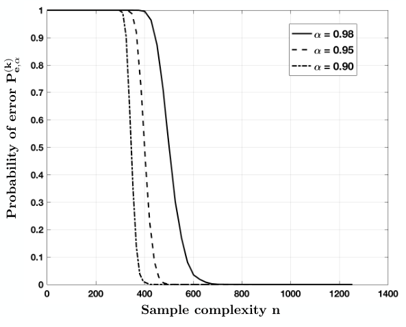
In Fig. 4, we observe the effect of on the sample complexity for a fixed query difficulty (D=6). For the almost exact recovery, we claim that the recovery is reliable when or more of the variables are recovered with high probability. We plot for for and show that the required to make close 0 increases as the value of increases.
VI Conclusions
We have proposed a method for designing a sequence of parity queries to recover the binary variables with high probability at the optimal sample complexity (up to constant factors) in a response model where only a randomly selected subset of the queries is answered. In particular, defining the query difficulty as the average size of the query subsets we analyzed the fundamental trade-offs between recovery accuracy , query difficulty and sample complexity . We considered two recovery conditions, exact recovery and almost exact recovery with fraction for , and showed that for exact recovery it is necessary and sufficient to have the sample complexity and for almost exact recovery the sample complexity for constants . We also provided a query-degree distribution for which the BP decoding process can guarantee the almost exact recovery of variables at the optimal sample complexity.
There are several interesting future research directions related to this work. One direction is to relax the assumption so as to tolerate poor reconstruction of a larger fraction of variables. In particular, we can consider extending Theorem 2 and Theorem 3 on almost exact recovery to the partial recovery problem where some smaller fraction of the variables are to be recovered, e.g., . An interesting question is whether it is possible to recover a smaller number of variables with only measurements even with a very low query difficulty , which does not increase in . Recall that in the exact recovery problem the query difficulty required a sample complexity of .
Another interesting direction is to apply the proposed parity-based query design to a more general measurement model with applications in crowdsourcing systems where workers may provide incorrect answers. For real crowdsourced labeling problems the probability that a worker provides an incorrect answer changes depending on the query difficulty. Designing querying schemes that minimize the sample complexity in recovering the attributes of objects under such a noisy model is a worthwhile problem for future study.
Appendix A Proof of Lemma 1
To prove this lemma, we refer to the similar bound provided in [26].
Lemma 8
Let and . Then we have
| (87) |
Note that
| (88) |
Therefore, by using Lemma 8, we can find an upper bound on as a scaling of of the form
| (89) | ||||
Define
| (90) |
We first consider the case (i.e., ). Since attains its maximum at or , we find that
Hence, and the last case in (89) is irrelevant.
- 1.
For (or, ),
Note that . Since is an decreasing function of , if then . Thus,
(91) - 2.
For (or, ),
Proceeding as above, we get
(92)
In the case , we can obtain the bounds for simply by changing to .
Appendix B Proof of Lemma 2
When the maximum query degree for some , the bound in (30) can be simplified as
| (93) |
When we plug in the sample complexity or some , the bound becomes
| (94) |
When , we can bound the term in the summation as
| (95) |
where the first inequality follows from and from for and , and the second inequality is true for for any constant .
When , we can bound the term in the summation as
| (96) |
where the first inequality is from , and the second inequality follows from , , and for . The last inequality is from for with .
Appendix C Proof of Lemma 3
In this lemma, we prove an upper bound on where
| (97) |
For the soliton distribution
we have the query difficulty
For simplicity, here we assume that . Recall that
| (98) |
which is a decreasing function of , and for .
- 1.
If ,
Thus, if ,
- 2.
If , we first notice that
(99) Thus and . In this case,
(100) Moreover, since , if for some sufficiently large , ( suffices)
(101) From Stirling’s formula, we also have that
hence
(102) Thus, if ,
(103) Note that
(104) - 3.
- 4.
If ,
(107) Thus, if ,
(108)
Appendix D Proof of Lemma 6
In this lemma, we show that for , we have
| (109) |
for a constant .
By definition,
| (110) |
If , then , which makes the analysis different from Proposition 10 of [19]. However, if , then anyway, and we can use Proposition 10 of [19] to find that
| (111) |
If , this proves the desired lemma. However, in our case since and . To find the lower bound on for , we use the following lemma.
Lemma 9
For any positive integers ,
| (112) |
Proof:
For any fixed , we prove the lemma by induction on . For , it obviously holds since both sides are equal to . Suppose that the formula holds for . Then, for , and
| (113) |
This proves the desired lemma. ∎
We now compute for . Since
| (114) |
we find that
| (115) |
where we used Lemma 9 to get the last line. Thus,
| (116) |
This in particular shows that is an increasing function of . Thus, we get
| (117) |
To estimate the right-hand side, we notice that
| (118) |
In particular,
| (119) |
for a constant .
References
- [1] H. W. Chung, J. O. Lee, and A. O. Hero, “Fundamental limits on data acquisition: Trade-offs between sample complexity and query difficulty,” in 2018 IEEE International Symposium on Information Theory (ISIT). IEEE, 2018, pp. 681–685.
- [2] H. W. Chung, J. O. Lee, D. Kim, and A. O. Hero, “Trade-offs between query difficulty and sample complexity in crowdsourced data acquisition,” in 2018 56th Annual Allerton Conference on Communication, Control, and Computing (Allerton). IEEE, 2018, pp. 639–646.
- [3] D. R. Karger, S. Oh, and D. Shah, “Budget-optimal task allocation for reliable crowdsourcing systems,” Operations Research, vol. 62, no. 1, pp. 1–24, 2014.
- [4] M. S. Bernstein, J. Brandt, R. C. Miller, and D. R. Karger, “Crowds in two seconds: Enabling realtime crowd-powered interfaces,” in Proceedings of the 24th annual ACM symposium on user interface software and technology. ACM, 2011, pp. 33–42.
- [5] D. J. MacKay, “Information-based objective functions for active data selection,” Neural Computation, vol. 4, no. 4, pp. 590–604, 1992.
- [6] B. Settles, “Active learning literature survey,” University of Wisconsin, Madison, vol. 52, no. 55-66, p. 11, 2010.
- [7] D. V. Lindley, “On a measure of the information provided by an experiment,” The Annals of Mathematical Statistics, pp. 986–1005, 1956.
- [8] V. V. Fedorov, Theory of optimal experiments. Elsevier, 1972.
- [9] E. Abbe and C. Sandon, “Community detection in general stochastic block models: Fundamental limits and efficient algorithms for recovery,” in Foundations of Computer Science (FOCS), 2015 IEEE 56th Annual Symposium on. IEEE, 2015, pp. 670–688.
- [10] B. Hajek, Y. Wu, and J. Xu, “Information limits for recovering a hidden community,” IEEE Transactions on Information Theory, 2017.
- [11] C. E. Tsourakakis, M. Mitzenmacher, K. G. Larsen, J. Błasiok, B. Lawson, P. Nakkiran, and V. Nakos, “Predicting positive and negative links with noisy queries: Theory & practice,” arXiv preprint arXiv:1709.07308, 2017.
- [12] A. Mazumdar and S. Pal, “Semisupervised clustering, and-queries and locally encodable source coding,” in Advances in Neural Information Processing Systems, 2017, pp. 6489–6499.
- [13] P. W. Holland, K. B. Laskey, and S. Leinhardt, “Stochastic blockmodels: First steps,” Social networks, vol. 5, no. 2, pp. 109–137, 1983.
- [14] E. Abbe and A. Montanari, “Conditional random fields, planted constraint satisfaction and entropy concentration,” in Approximation, Randomization, and Combinatorial Optimization. Algorithms and Techniques. Springer, 2013, pp. 332–346.
- [15] D. Zhou, J. Huang, and B. Schölkopf, “Learning with hypergraphs: Clustering, classification, and embedding,” in Advances in neural information processing systems, 2007, pp. 1601–1608.
- [16] S. Agarwal, K. Branson, and S. Belongie, “Higher order learning with graphs,” in Proceedings of the 23rd international conference on Machine learning. ACM, 2006, pp. 17–24.
- [17] G. Karypis and V. Kumar, “Multilevel k-way hypergraph partitioning,” VLSI design, vol. 11, no. 3, pp. 285–300, 2000.
- [18] J. Leskovec, D. Huttenlocher, and J. Kleinberg, “Predicting positive and negative links in online social networks,” in Proceedings of the 19th international conference on World wide web. ACM, 2010, pp. 641–650.
- [19] M. Luby, “LT codes,” in Proceedings of The 43rd Annual IEEE Symposium on Foundations of Computer Science, 2002. IEEE, 2002, pp. 271–280.
- [20] D. Achlioptas and A. Coja-Oghlan, “Algorithmic barriers from phase transitions,” in 2008 49th Annual IEEE Symposium on Foundations of Computer Science. IEEE, 2008, pp. 793–802.
- [21] H. Haanpaa, M. Jarvisalo, P. Kaski, and I. Niemela, “Hard satisfiable clause sets for benchmarking equivalence reasoning techniques,” Journal on Satisfiability, Boolean Modeling and Computation, vol. 2, pp. 27–46, 2006.
- [22] M. Ibrahimi, Y. Kanoria, M. Kraning, and A. Montanari, “The set of solutions of random xorsat formulae,” THE ANNALS of APPLIED PROBABILITY, pp. 2743–2808, 2015.
- [23] E. Abbe, A. S. Bandeira, A. Bracher, and A. Singer, “Decoding binary node labels from censored edge measurements: Phase transition and efficient recovery,” IEEE Transactions on Network Science and Engineering, vol. 1, no. 1, pp. 10–22, 2014.
- [24] A. Mazumdar and B. Saha, “Clustering with noisy queries,” in Advances in Neural Information Processing Systems, 2017, pp. 5788–5799.
- [25] A. Dembo, A. Montanari et al., “Finite size scaling for the core of large random hypergraphs,” The Annals of Applied Probability, vol. 18, no. 5, pp. 1993–2040, 2008.
- [26] K. Ahn, K. Lee, and C. Suh, “Community recovery in hypergraphs,” IEEE Transactions on Information Theory, 2019.
- [27] O. Watanabe, “Message passing algorithms for mls-3lin problem,” Algorithmica, vol. 66, no. 4, pp. 848–868, 2013.
- [28] D. J. MacKay, “Fountain codes,” IEE Proceedings-Communications, vol. 152, no. 6, pp. 1062–1068, 2005.
- [29] A. Shokrollahi, “Raptor codes,” IEEE Transactions on Information Theory, vol. 52, no. 6, pp. 2551–2567, 2006.
- [30] D. Du, F. K. Hwang, and F. Hwang, Combinatorial group testing and its applications. World Scientific, 2000, vol. 12.
- [31] G. K. Atia and V. Saligrama, “Boolean compressed sensing and noisy group testing,” IEEE Transactions on Information Theory, vol. 58, no. 3, pp. 1880–1901, 2012.
- [32] M. Cheraghchi, A. Hormati, A. Karbasi, and M. Vetterli, “Group testing with probabilistic tests: Theory, design and application,” IEEE Transactions on Information Theory, vol. 57, no. 10, pp. 7057–7067, 2011.
- [33] R. Dorfman, “The detection of defective members of large populations,” The Annals of Mathematical Statistics, vol. 14, no. 4, pp. 436–440, 1943.
- [34] I.-H. Wang, S.-L. Huang, K.-Y. Lee, and K.-C. Chen, “Data extraction via histogram and arithmetic mean queries: Fundamental limits and algorithms,” in 2016 IEEE International Symposium on Information Theory (ISIT). IEEE, 2016, pp. 1386–1390.
- [35] A. E. Alaoui, A. Ramdas, F. Krzakala, L. Zdeborová, and M. I. Jordan, “Decoding from pooled data: Sharp information-theoretic bounds,” SIAM Journal on Mathematics of Data Science, vol. 1, no. 1, pp. 161–188, 2019.
- [36] T. M. Cover and J. A. Thomas, Elements of information theory. John Wiley & Sons, 2012.
- [37] I. Csiszar and J. Körner, Information theory: coding theorems for discrete memoryless systems. Cambridge University Press, 2011.