Global search for localised modes in scalar and vector nonlinear Schrödinger-type equations
Abstract
We present a new approach for search of coexisting classes of localised modes admitted by the repulsive (defocusing) scalar or vector nonlinear Schrödinger-type equations. The approach is based on the observation that generic solutions of the corresponding stationary system have singularities at finite points on the real axis. We start with establishing conditions on the initial data of the associated Cauchy problem that guarantee the formation of a singularity. Making use of these sufficient conditions, we identify the bounded, nonsingular, solutions — and then classify them according to their asymptotic behaviour. To determine the bounded solutions, a properly chosen space of initial data is scanned numerically. Due to asymptotic or symmetry considerations, we can limit ourselves to a one- or two-dimensional space. For each set of initial conditions we compute the distances to the nearest forward and backward singularities; large or indicate the proximity to a bounded solution. We illustrate our method with the Gross-Pitaevskii equation with a -symmetric complex potential, a system of coupled Gross-Pitaevskii equations with real potentials, and the Lugiato-Lefever equation with normal dispersion.
Keywords:
nonlinear mode, soliton, blow up, defocusing nonlinear Schrödinger equation, Gross-Pitaevskii equation, Lugiato-Lefever equation1 Introduction
The aim of this paper is to formulate a new approach to the determination of localised solutions of the nonlinear Schrödinger-type systems. The method is particularly efficient in situations where localised solutions are not unique; it aims at finding all solutions coexisting for a given set of parameter values. The new approach applies to a broad variety of scalar and vector equations, autonomous or not. We start with providing several examples of physical significance.
1. The Gross-Pitaevskii equation,
| (1) |
describes the ground state of the quantum system of identical bosons in the mean field approximation [1]. Equation (1) is written in its dimensionless form, and corresponds to the elongated (“cigar-shaped”) condensate with repulsive interparticle interactions. In (1), is a complex-valued function whose real part represents the confining potential. The imaginary part accounts for the injection and elimination of atoms in the condensate in the region where is positive and negative, respectively.
Assuming a steady state solution of the form , equation (1) reduces to a nonlinear ordinary differential equation
| (2) |
It is well-known that even in the case of a real potential (parabolic or periodic) and real amplitude , equation (2) can describe numerous nonlinear structures. These include bright and dark solitons [2, 4, 3, 5, 6, 7, 8, 9, 10, 11, 15], nonlinear periodic structures [8, 12], domain walls [13], gap waves [14] and even more complex multi-soliton structures that can be classified by means of some coding procedure [17].
The situation becomes even more involved when the potential is complex. One of the notable realisations here is concerned with condensates in parity-time ()-symmetric potentials [18, 19, 20, 21]. In this case is an even function, i.e., and is odd, . Another area where equation (1) with a -symmetric potential finds applications, is nonlinear optics. In optics, describes the complex-valued refractive index of a defocusing waveguide, where domains with positive and negative imaginary part of correspond to gain and loss of energy, respectively [22]. A wide variety of optical potentials has been considered, see e.g. [23, 24, 25, 26, 27, 28] for particular examples and [21, 29, 30] for recent reviews.
Decomposing into its real and imaginary parts, , we write (2) as a system
| (3) | ||||
| (4) |
Complete description of all coexisting localised modes described by (3)-(4) is a complex problem that generically remains unsolved.
2. The dynamics of a mixture of two Bose-Einstein condensates (without the injection or elimination of atoms) is described by the coupled Gross-Pitaevskii equations
| (5) | ||||
| (6) |
(See, e.g. the recent review [31]). Here are the macroscopic wavefunctions of the condensates, characterize the inter-atomic collisions, and the real function describes the trap potential. The generalisation to the case of three or more condensates is straightforward.
It is worth noting that equations (5)-(6) emerge in the optical context as well. In optics, this system describes the propagation of two light beams in the presence of cross-phase modulation [32].
The list of known localised solutions of this system comprises the nodeless vector solitons (aka ground states or bright-bright solitons) [73, 72, 68]; their dark-bright [75, 76, 71, 65, 66], dark-dark [67, 77, 78], and dark-antidark [74] counterparts, as well as localised solutions with more complex structure [68].
One of the applications of the system (5)-(6) is to the description of the miscibility-immiscibility transition (MIT) in a binary Bose–Einstein condensate. As the inter-species coefficient is increased through a critical value, the mixed components separate. A simple qualitative estimate for the threshold is [79, 70] — although this expression is known not to be exact [69].
The substitution with real , takes (5)-(6) to the following system:
| (7) | ||||
| (8) |
The MIT transition corresponds to the symmetry-breaking bifurcation of its ground state solution. In order to seek for new localised solutions and study bifurcations of the known ones, it is useful to have a global picture of the phase space of the system (7)-(8) at a given set of parameter values. This global view should include all nonlinear modes determined so far.
3. The externally driven nonlinear Schrödinger equation (also known as the Lugiato-Lefever equation),
| (9) |
arises as an amplitude equation for an optical pulse in the pumped ring resonator [42]. Here is a complex amplitude of the field in the resonator, while and stand for the damping coefficient and pumping amplitude, respectively. The studies of the Lugiato-Lefever equation were boosted by the discovery of the frequency combs associated with the Kerr temporal solitons (see e.g. [45, 46, 47]). The frequency combs are of the utmost importance for the metrology applications [43, 44].
Equation (9) is written in its dimensionless form. The control parameters and are real; the negative and positive sign in front of the cubic term corresponds to the case of normal and anomalous dispersion, respectively. Assuming that the field is stationary and decomposing , equation (9) is cast in the form
| (10) | ||||
| (11) |
A variety of solutions of (10)-(11) have been reported in literature. These include bright and dark solitons [55, 56, 57, 58, 59, 47, 52, 53] as well as periodic structures [49, 50]. For particular values of the control parameters, there are kinks interpolating between different flat backgrounds [52, 53]. As a parameter is varied, a bright soliton may transform into a kink-antikink pair [53, 51], with the transformation involving the snaking mechanism [64]. Heteroclinic connections between a periodic solution and a flat background were found in the case of the anomalous dispersion [49] and it was conjectured [52] that no such connections exist in the case of the normal dispersion. (In what follows we argue that the connections of the above type do exist in some parameter range).
Equations (2), (7)-(8) and (9) admit a common vector formulation:
| (12) |
Here is an -component real vector of unknowns, ; is an real matrix-valued function of ; is a diagonal real matrix where the entries , , are bilinear forms of -component vectors and , with the coefficients dependent on ; is an -component real vector-function. In this study we focus on soliton solutions of (12). These are localised solutions satisfying the boundary conditions
| (13) |
where are constant vectors.
Typically, a numerical search for soliton solutions involves an iterative algorithm with some initial guess for the form of the soliton. Since the system (12) is nonlinear, it is not a priori obvious whether the resulting solution is unique, and if not — how to set up initial guesses leading to other solutions coexisting for the same set of parameters. A method providing a global view of all coexising solitons would therefore be of great help.
In this paper, we formulate a variant of the shooting method aimed to give a comprehensive description of the full set of localised solutions of the system (12) with the defocusing nonlinearity. The method is based on the observation that, under some physically meaningful assumptions about the coefficients and potential functions of the system (12), most of its solutions become infinite at a finite . We formulate conditions that allow one to recognise a singular solution before it blows up. Using these conditions we estimate the distance to the singularities and seek for bounded solutions in the vicinity of solutions with “anomalously large” . The set of bounded solutions contains, in particular, all solitons — that is, localised solutions with the boundary conditions (13).
The paper is organised as follows. The basics of our method are outlined in Section 2. We demonstrate that the singular behaviour is generic for equations in the class (12), formulate sufficient conditions for the blow-up and establish an upper bound for the distance to the singularity. In Sections 3,4 and 5 the method is exemplified by the -symmetric complex Gross-Pitaevskii equation (1), the system (5)-(6) of two real Gross-Pitaevskii equations, and the Lugiato-Lefever equation (9). Section 6 concludes the paper with a summary and discussion.
2 The method
2.1 Singular solutions
A simple example of an equation with the required properties is
| (14) |
This is a particular case of the Emden-Fowler equation [33]. It results by setting , , , and in the system (12) with . The general solution of (14) is a union of two bi-parametric families,
| (15) |
and
| (16) |
where , is real and , , are the Jacobi elliptic functions. An additional one-parameter family arises by sending in (15),
| (17) |
while sending in (16) produces the trivial solution .
Since the denominator in the expressions for has zeros, none of the solutions (15), (16) or (17) is free from singularities. (The only nonsingular solution is .) The ingredient in (14) that is responsible for the blow-up of solutions, is the repulsive (defocusing) nonlinear term . Indeed, any solution of the linear equation or the equation with the attractive (focusing) term exists globally in the whole real axis .
The singular solutions continue to prevail if we consider the following well-researched generalisation of the Emden-Fowler equation:
| (18) |
The singular solutions are typical for the case , . (See [34], Theorem 20.30.)
Another generalisation is given by the equation
| (19) |
with several classes of real . As in the previous examples, most of the solutions of (19) with the initial conditions set at some , blow up on the real line. In the case of the parabolic and infinite double-well potentials , the singular behavior of solutions to (19) was exploited to classify all localised bounded modes coexisting for the given [15]. In the case of the periodic potentials, the blowing up solutions are also generic [16]. This fact gives rise to the classification of nonlinear structures in terms of bi-infinite symbolic sequences [17, 16, 39].
2.2 Blow-up in the system (12): sufficient conditions
In fact, the singular behaviour is generic even in a vector situation, with a broad class of nonlinear terms in the system (12). The blow-up can be guaranteed if the initial condition of the corresponding Cauchy problem is simply “large enough". The following proposition makes this notion precise.
Proposition 1. Assume the following.
- (i)
is a continuous matrix function defined on , and there exists a constant such that for any and any ,
(20) Hereafter .
- (ii)
Any entry , , of the diagonal matrix is a positive definite quadratic form of . Moreover, , , is a continuous function of , defined in for any , and there exists a constant such that for any , any , and any ,
(21) - (iii)
is a continuous function of defined on , and there exists a constant such that for any ,
(22)
Then the solution of the Cauchy problem for Eq. (12) with initial data , such that
| (23) | ||||
| (24) |
blows up, i.e. for some . Moreover, where
| (25) |
The proof of Proposition 1 is relegated to A.
Four comments are in order.
1. Proposition 1 states that, under certain conditions on , and , , the solution of the system (12) with initial conditions at has a singularity within the positive -neighbourhood of . If the assumptions (i)-(iii) are met by the coefficient matrices , and vector , with , a singularity is guaranteed to occur within the negative -neighbourhood.
2. The initial conditions for the Cauchy problem in Proposition 1 are set at . However, by shifting the initial conditions can be imposed at any point . Then Proposition 1 guarantees the presence of singularities of the solution in the positive -neighbourhood of .
2.3 Numerical approach
Any solution of the system (12) is uniquely determined by initial conditions imposed at some point :
| (28) |
Let be the coordinate of the singularity of the solution to the Cauchy problem (12), (28) located to the right of . Similarly, let be defined as the coordinate of the singularity to the left of . If the solution of the Cauchy problem exists in the whole semi-infinite interval , we write
| (29) |
Similarly, if the solution exists in the whole semiaxis , we let
| (30) |
The definition of the functions is illustrated in Fig. 1.
Our aim is to detect points in the space , where equations (29) and (30) hold true — that is, detect the initial conditions for which the solution exists on the whole real line. Note that the validity of (29) and (30) does not yet imply that is a soliton solution of Eq. (12). One still needs to check whether the boundary conditions (13) are satisfied.
In order to compute numerically for initial data we choose the value large enough, such that
where is a small tolerance value chosen beforehand. For a given set of and , , we solve the Cauchy problem (12), (28) along the -line. Let reach a point where the solution satisfies the conditions and . Then according to Proposition 1, approximates the position of the singularity up to the error . In a similar manner the value of can be computed.

Then the approach can be sketched in general as follows. Introduce a fine grid in the space of parameters , . For each point of the grid we compute the values . If at some node of the grid the values of are “anomalously large”, we repeat the procedure on a finer grid in the vicinity of this node. Repeating in such a way we can locate the initial data , that correspond to the bounded solution.
Evidently, the scanning in the space of parameters , with large is a computationally costly exercise. However, the dimension of the space may be reduced by noting a symmetry of the nonlinear mode or using its asymptotic behaviour at infinity.
(a) Symmetry-based reduction. The former approach can be exemplified by the Gross-Pitaevski equation (2) with a -symmetric potential . It is known that all soliton solutions supported by a generic potential of this type have to be symmetric [21]. This implies that while studying the system (3)-(4) one can impose the conditions and and analyze functions of two arguments rather than four: and . Plotting the function over -plane we identify the initial values corresponding to the infinite interval of existence of the solution to the Cauchy problem. (On the other hand, we do not need to plot the function since its graph obtains from the graph of by a mere reflection , .) Once the solutions existing over the entire real line have been identified, their asymptotic behaviours as should be further examined to select solitons.
(b) Asymptotic reduction. An alternative approach is suitable for solutions of the system (12) approaching the equilibrium state as (or the equilibrium state as ). In the phase space of the dynamical system generated by equations (12), the corresponding trajectories lie on the stable/unstable manifold of this equilibrium state. Accordingly, we can restrict ourselves to the evaluation of the function (or ) just on that manifold. If the dimension of the stable manifold is much smaller than , this reduction will simplify the analysis quite considerably.
To illustrate this idea, we consider the linearisation of the system (12) about the equilibrium state :
| (31) |
Here is an real matrix. Assume that the equation (31) has linearly independent solutions satisfying as and . Any solution of the vector equation (12) approaching as , can be approximated by
| (32) | |||
| (33) |
Here are real coefficients. We examine the solution of the system (12) with the initial conditions (32)-(33) imposed at a point with a large . When , one can plot the function over an interval . When , the function can be plotted over a box . The objective is to determine the values of the coefficients giving rise to “anomalously” large negative . These values correspond to large (potentially infinite) intervals of existence of the solution of the Cauchy problem. The resulting set of solutions should then be classified into (a) solitons and (b) nonlocalised bounded modes, such as periodic and quasiperiodic structures, flat-periodic connections etc.
3 The -symmetric Gross–Pitaevskii equation
In this and the next two sections, our method is illustrated by several systems of physical significance. We start with the -symmetric Gross-Pitaevskii equation. The stationary states of the Gross-Pitaevskii model satisfy the system (3)-(4). The system (3)-(4) belongs to the general class (12) with and
If is bounded from below, the assumptions of Proposition 1 are met, with
According to (26), solutions of the system (3)-(4) with the initial conditions set at and satisfying
| (34) | ||||
| (35) |
blow up. The coordinate of the blow-up point is estimated as
| (36) |
We exemplify our approach for -symmetric harmonic oscillator defined by
| (37) |
where is a real parameter. In this case, . Two versions of the approach mentioned in Section 2.3 are applicable.
3.1 Symmetry-based approach
The harmonic potential is generic in the sense that it only supports -symmetric solutions. These have even and odd ; consequently, and . The -symmetric solutions are characterised by the initial data and . (See the discussion in Sec. 2.3).
A numerically generated plot of the function for and is presented in Fig. 2. In order to obtain this figure, the subset of the plane was sampled with small enough increments in and . (Specifically, we used ). The Cauchy problem was solved using a Runge-Kutta routine with the step size . The numerical value of was computed by detecting the point on the real axis where the absolute value of exceeded a large enough value chosen beforehand. Specifically, we took ; in view of the bound (36) the resulting value of is accurate to within . No further accuracy improvement is possible without the Runge-Kutta stepsize reduction.
In the plot shown in Fig. 2, five separate peaks are clearly distinguishable. One of these corresponds to the trivial solution while the other four peaks correspond to localised nonlinear modes. The nontrivial solutions form two pairs symmetric with respect to the origin on the -plane: . This symmetry stems from the invariance of the equation (2) under the transformation . Accordingly, the parameter sets and can be regarded equivalent.
The coordinates of a peak of provide an estimate for the location of the corresponding bounded solution. Once an approximate location of the peak is known, one can scan its neighbourhood with smaller step sizes , , so as to determine the location more accurately. The resulting values of and are then used to compute the bounded solution. The solutions associated with two nonequivalent peaks in Fig. 2 are shown in Fig. 3.


3.2 Asymptotics-based approach
An alternative approach to localised solutions of the equation (2) with the oscillator potential (37) exploits the asymptotic behaviour of the solution rather than its symmetry. Instead of assuming that the nonlinear mode is symmetric, we require it to be localized,
| (38) |
Due to boundary condition (38) the asymptotics of at is determined by the linearised equation
Then the behaviour of at is described by the asymptotic of the parabolic cylinder functions [81]
| (39) |
where is a constant and the parameter of the potential (37). We impose the initial condition at the point , with a large negative . The value of is set to (39) and the value of to the dominant term in the derivative of (39):
| (40) |
In view of the U(1) symmetry of the stationary Gross-Pitaevskii equation (2), it is sufficient to consider only real positive . Indeed, the solution corresponding to a complex is related to the solution with real positive by the phase rotation .
For a generic , the solution with the initial conditions (40) blows up at some finite point . Thus the search for localised nonlinear modes reduces to finding the special values of in (40) that produce solutions remaining bounded on the entire line.
In our numerics we used . Figure 4 shows the numerically generated dependencies with and twenty-one equidistant values of between 0 and 1. Each curve with far enough from 1 features two separate spikes. The analysis of the shapes of the corresponding solutions confirms that each pair of spikes does represent a pair of nonequivalent localised -symmetric modes. (We have already determined these modes in the previous subsection using the symmetry approach.) As is increased, the two spikes (two modes) merge and disappear.

4 The coupled Gross-Pitaevskii equations
Our second example is the system of coupled Gross-Pitaevskii equations (5)-(6). This system also can be cast into the form (12) with
The problem that we address using our approach, can be formulated as follows. Let the parameters and be assigned certain values. For this particular choice of parameters, provide a global description of the set of all localised solutions of the system (7)-(8).
For illustrative purposes we take the harmonic trapping potential: . Normalising the coefficients and to unity, we assume that the remaining parameters satisfy , . The system (7)-(8) verifies the assumptions of Proposition 1 with and .
Consider a class of solutions defined by their behaviour at the left infinity:
The full asymptotic behaviour, as , of any solution in is straightforward from the linear part of the system (7)-(8):
| (41) |
where are real constants. Conversely, for any choice of real and , there is a unique solution of (7)-(8) with the behaviour (41) [80].
Typically, solutions from blow up at a finite point. We introduce the function that returns the point of blow up for the solution in , parametrised by the pair . A plot of the function can be obtained by scanning a portion of the plane , with and being kept fixed. Since the system (7)-(8) is invariant under and , only the quadrant needs to be scanned.
Our numerical study proceeded by introducing a radial grid in the plane. Having picked a large negative , we solved numerically the Cauchy problem with the initial data (41) applied at for each point of this grid.
According to Proposition 1 and comment 3 after this, we would terminate the numerical run once the condition (24)
was satisfied and exceeded a large positive threshold ,
chosen beforehand. The corresponding value of , , gives an approximation for the blow up point . The error of the approximation is bounded by equation (27):
The values of and were chosen so large that any further increase of these parameters did not have any visible effect on the resulting plot of .

A typical graph of the function is in Fig. 5. The following comments are in order.
1. The peak at corresponds to the trivial solution of the system (7)-(8). The two pairs of peaks on the and axes correspond to solutions with one of the two components equal to zero. For instance, the peaks on the -line correspond to solutions with and , where solves the equation
| (42) |
One of these solutions is even and nodeless (the bright soliton), and the second one is odd and has exactly one node at (the dark soliton). We call these solitons the single-component solitons and mark them and . The peaks on the -line correspond to the single-component solitons and . These solutions are sketched in the insets to Fig. 5.
2. The two peaks on the bisector line correspond to solutions with , where satisfies
These solutions can be labelled as the bright-bright and dark-dark solitons and denoted and , respectively. The components of the soliton are even functions of and those of the soliton are odd.
3. There are two peaks that do not belong to any of the above-mentioned cases. These can be classified as mixed states of dark-bright or bright-dark type and labelled as and , respectively.
4. Refining the grid and expanding the scanned area does not reveal any new peaks in the graph. We accept this as numerical evidence of the nonexistence of any additional soliton solutions with and for the given values of and . The localised modes with negative , or both, are related to those discussed above by reflections and . For example, the mixed state gives rise to three solutions with negative , or both. These will be denoted , and .
Using our method, we track bifurcations of the solitons occurring as is varied while is kept constant. It is convenient to illustrate these bifurcations using just the positive quadrant of the plane; see Fig. 6. The peaks corresponding to the soliton states are marked by red dots. As is changed, the solitons undergo the following transformations.

a) When (Fig. 6(a)) the equations are uncoupled. There are four nonequivalent single-component solitons (marked by circles on the and axes): , , and . Also there are four mixed states , , and .
b) As is increased (Fig. 6(b-c)), the points that mark the and states move toward the and axes, respectively. Once the parameter has reached , the solution is absorbed by the single-component state and the is absorbed by (see the diagram 7, panel a). Note that the symmetric states and are also absorbed by and ; therefore the bifurcations are of the pitchfork type here.
c) Six soliton states , , , , , persist in the interval . No other localised solutions were found in this range of .
d) At the point , the system possesses an additional continuous symmetry. If is a solution of the equation (42), the vector function with satisfies the system (7)-(8). This degeneracy explains the diagram in Fig. 6(d) where the pairs of pertaining to localised states form two circular arcs. The arc of the smaller radius connects the and states, whereas the longer arc connects to .
e) When is in the range , with , we have the same six soliton states again: , , , , , and . [See Fig. 6(e)]. A symmetry-breaking pitchfork bifurcation occurs as goes through . Here, two asymmetric states and branch off from the solution [Fig. 6(f)]. The emerging states are related to each other by the inversion supplemented by the transposition , (see Fig.7, panel b). This bifurcation corresponds to the MIT transition and has been widely discussed in the literature.
f) As is raised further, the -points for the asymmetric states and move closer to the and axes — but never reach them. The eight soliton states persist until the next bifurcation point , with [Fig. 6(g)].
g) On passing through a new pitchfork bifurcation takes place. Here, two pairs of dark-bright solitons with small bright components branch off from the single-component dark solitons and [Fig.6(h)]. The pair detaching from the has opposite lower components; we denote these states , see Fig.7, panel c. The pair bifurcating from the comprises solitons with opposite upper components: . See Fig. 6(i).
h) One more pitchfork bifurcation occurs as passes through . Here, two states branch off from the solution. The new states that we denote by and , are related by permutation: , . Both of their components are even and the solutions are of the bright-bright variety, see Fig.7, panel d.

Thus, our approach allows us to classify all solitons with and track their bifurcations in the interval . The bifurcations are summarised in Fig. 7. It is fitting to note that the bifurcation sequence for the solitons is well protocoled in the literature. (See e.g. Fig. 11 in [68]). On the other hand, the homotopy connection between the and states (and its symmetric to counterpart), to the best of our knowledge, have not been reported before. Neither we have been not aware about the pitchfork bifurcations of the and .
5 The Lugiato-Lefever equation
Our third example is the externally driven damped nonlinear Schrödinger equation — equation (9). For the stationary states , the equation can be written as
| (43) | ||||
| (44) |
The negative and positive signs in front of the nonlinearity correspond to normal and anomalous dispersion, respectively.
In the four-dimensional phase space with coordinates equations (43)-(44) generate a reversible dynamical system. (The system is conservative if ; otherwise, to the best our knowledge, it does not have any first integral.) Homogeneous solutions — often referred to as the flat backgrounds — correspond to equilibria of the dynamical system, and periodic solutions correspond to its closed orbits. Solutions that are asymptotic to the same respectively different backgrounds as and , represent homoclinic respectively heteroclinic orbits. There is a great body of work devoted to the closed orbits as well as homoclinic and heteroclinic solutions in reversible systems, see [60, 62, 63, 64]. Methods for the determination of such trajectories are also well documented [61].
In the case of the normal dispersion, the system
| (45) | ||||
| (46) |
satisfies the assumptions of Proposition 1 of section 2.2. In this case , and , so that if
the solution of the Cauchy problem with the initial conditions at blows up at some point within the left -neighbourhood of where
The homogeneous solutions of (45)-(46) are , where the constants satisfy the algebraic system
| (47) | ||||
| (48) |
Depending on the values of and , the system (47)-(48) may have one or three roots [56, 57]. The type of the equilibrium is determined by the eigenvalues of the linearisation matrix
where
Since the dynamical system (43)-(44) is reversible, it may have four types of equilibria. (i) If the eigenvalues are both real and positive, the equilibrium is classified as a saddle. (ii) Real negative corespond to an elliptic point. (iii) Two real eigenvalues of the opposite sign define a saddle-center. (iv) Finally, an equilibrium with the complex conjugate eigenvalues, is a saddle-focus. Fig. 8 divides the -plane into four parameter regions according to the number of equilibria and their types.

Generic localised solutions of (43)-(44) are asymptotic to the flat backgrounds of the saddle and saddle-focus types. To illustrate our method, we restrict ourselves to the case of the saddle-focus and denote the associated pair of complex eigenvalues of .
In the vicinity of the saddle-focus equilibrium, there exist a local 2D stable manifold, , and a local 2D unstable manifold, . We parametrise trajectories on as follows. Let and define , with , such that . The asymptotic behaviour of a solution of (43)-(44) that tends to as is
| (49) | ||||
| (50) |
Here while and are free parameters.
Consider the Cauchy problem for the system (43)-(44) with the initial data on :
| (51) | ||||
| (52) | ||||
| (53) | ||||
| (54) |
where and is a fixed positive value that has to be taken small enough. In (51)-(54) we have used the translation invariance to set the initial condition at . Since is fixed, the parameter defines the trajectory on uniquely. See Fig. 9.
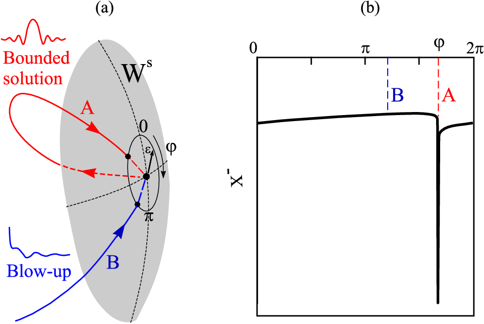
Let denote the coordinate of the singularity of the solution with the asymptotic behaviour (49)-(50) as . Clearly, depends on the parameter . (See the schematic in Fig. 9.) The graph of the function for is constructed by solving the system (43)-(44) in negative , with the initial data (51)-(54). The value of is approximated by the coordinate of the point on the real axis where exceeds a threshold set beforehand. The accuracy of this approximation is given by in equation (25).
We now present results of the computations for and three values of .
5.1 The case , .
The function is depicted in Fig. 10. A coarse sampling of the interval reveals a single well; see panel (a). Panel (b) zooms in on the fine structure of that well. Here, one can discern numerous dips representing bounded solutions. Some of these solutions are illustrated in Fig. 11.


Several remarks are in order here.
1. Figure 10(b) gives only a rough idea of the fine structure of the well that is extremely complex. According to [63], the existence of the primary homoclinic orbit implies the existence of infinitely many homoclinic orbits that make loops in the vicinity of the primary orbit. These orbits correspond to bound states of solitons located some distance away from each other. This means that there are infinitely many dips that should be discernible by a sufficiently dense sampling.
2. Fig. 11 displays the Cauchy-problem solutions corresponding to some of the dips in Fig. 10(b). Most of these solutions blow up a certain distance away from the initial point. However this distance is large; hence Fig. 11 gives a fairly accurate description of the bounded solutions that remain close to the blowing-up solution over a long interval. (The former can be determined by the fine-tuning of ; see remark 4 below.) In particular, panel (a) of Fig. 11 gives an idea of the fundamental soliton of Eqs. (45)-(46). Panels (b)-(d) show a bound state of two fundamental solitons, with varied separation. (The existence of the bound states is due to the general argument in [63]; these solutions of the Lugiato-Lefever equation with normal dispersion have been reported in [52, 53]). Another type of localised mode — more precisely, a solution that remains close to such a mode — appears in panel (e). This solution deserves a special comment; see remark 5 below.
3. Panel (f) displays a heteroclinic connection between the saddle-focus equilibrium and a periodic orbit. This solution is novel. Although periodic solutions of the Lugiato-Lefever equation were reported in the literature [50], the connections between the flat and periodic solutions were only found in the equation with anomalous dispersion [49]. (In fact the heteroclinic connections of the said type were conjectured not to exist in the case of the normal dispersion [52].)
4. Even though generic solutions of the initial-value problem (43)-(44), (51)-(54) are unbounded, this one-parameter family does contain solitons and their complexes. The corresponding special parameter values can be determined in an algorithmic way.
Indeed, since the system is reversible, all trajectories that pass through the symmetry plane are symmetric. This means that the solution satisfying
and
for some , has to satisfy
as well. This observation suggests the following symmetrisation algorithm.
Let be fixed and , , , given by (51)-(54). We order zeros of the function , , so that
and define
Roots of the function lying in the neighbourhood of a “dip” of the function correspond to soliton solutions of the Lugiato-Lefever equation (45)-(46). These roots can be determined by the bisection method. Some profiles of soliton solutions obtained by this symmetrisation procedure are displayed in Fig. 12.
5. The heteroclinic connection between a periodic solution and the saddle-focus equilibrium gives rise to novel localised states with “locked” oscillations. A solution of this type is shown in Fig. 12 (d). This solution has been obtained by the symmetrisation procedure in the neighbourhood of the heteroclinic connection. (The above structure bears some similarity to the “truncated Bloch waves” of the Gross-Pitaevskii equation with a periodic potential [54].)

5.2 The case , .
The function with , has just one narrow dip; see Fig. 13 (a). Our numerical resolution was insufficient to discern any internal structure of this dip. The initial-value problem solution with the largest negative value of that we were able to reach, is shown in Fig. 13 (b). Making use of the symmetrisation algorithm in the neighbourhood of this solution we construct a localised nonlinear mode (Fig. 13 (c)). This soliton can be interpreted as a kink-antikink pair, where each of the kink and antikink connect the saddle and saddle-focus equilibria. Localised solutions of this type as well as the transition from the fundamental soliton to the kink-antikink pair by means of the “snaking” scenario, were discussed in [53].

5.3 The case , .
The function with , is shown in Fig. 14. As it does not feature any dips, we conclude that no bounded solutions exist in this case. As is increased, the function flattens out so that for large it is nearly a constant. This observation suggests that no soliton solutions asymptotic to the saddle-focus equilibrium exist for large values of .
A more detailed study of the novel nonlinear modes of the Lugiato-Lefever equation will be presented in a forthcoming publication.

6 Concluding remarks
In this paper, we have described a method for the numerical search and computation of localised solutions to a family of scalar or vector Schrödinger-type equations with the defocusing nonlinearity. Our method makes use of the fact that most of the solutions to the system (12) blow up a finite distance away from the initial point on the real line. It is, effectively, a procedure for the filtering out of the singular solutions. The procedure relies on a set of sufficient conditions for the blow up and an expression for an upper bound on the distance to the singularity. The sufficient conditions and the upper bound are derived in this paper.
Unlike iterative methods, our approach does not require any a priori details on the shape of solution that we seek to determine. As a result, the method is global: by scanning a sufficiently large domain in the space of initial values, we can obtain a comprehensive description of the set of coexisting localised modes. Its additional advantage is that it is capable of establishing the nonexistence of regular solutions to the boundary-value problem in question. If the nonlinear system does not have any localised modes, the method yields a “numerical evidence” of this fact.
We have illustrated our method with three examples. First, we used it to reproduce several results from literature on localised modes in the nonlinear Schrödinger equation with a complex-valued -symmetric potential. Second, we applied the new approach to a system of coupled Gross-Pitaevskii equations. Here, we have determined all coexisting soliton solutions in a chosen parameter range and tracked their bifurcations as the coupling parameter is varied. The third example concerned the Lugiato-Lefever equation with normal dispersion. In the latter case the method produces some novel solutions in addition to structures described in the literature. The new solutions include the heteroclinic connection between a periodic orbit and equilibrium state as well as a sequence of localised solutions consisting of several periods of oscillation connected to the equilibrium state on either side.
We close the paper by mentioning several theoretical and practical aspects of the method that deserve further investigation.
First, it would be instructive to fully understand properties of the functions that play the central role in the elimination of singular solutions. Under what conditions are these functions (a) well defined, (b) continuous, (c) differentiable, and (d) monotonic? Some results for particular cases can be found in [34, 35, 36, 37, 38].
Second, one should try to loosen the conditions (21) on the nonlinear term that guarantee the formation of a singularity. The result of [82] may be used to generalise the conditions (21) beyond the cubic defocusing nonlinearities. On the other hand, equations that have neither focusing nor defocusing nonlinearity but exhibit blowing up are not unheard of in the literature. For instance, most of the solutions to the equation
| (55) |
where is a real function with alternating sign, develop a singularity at a finite point in [40, 41]. With regard to the system (5)-(6), this suggests that our method may remain effective even for a much wider class of nonlinearities.
Finally, the present formulation of our approach confines it to the one-dimensional geometry. The method does not admit a straightforward generalisation to systems of the form (12) with replaced with . However it may be possible to extend it to quasi-one-dimensional situations, in particular to the radially-symmetric solutions in two and three dimensions.
Acknowledgments
Authors are grateful to A.D. Kirilin for his help with numerical work and fruitful discussions. GA and DZ were funded by Russian Science Foundation (Grant No. 17-11-01004). IB was supported by the National Research Foundation of South Africa (grants 105835, 85751 and 466082) and the European Union’s Horizon 2020 research and innovation programme under the Marie Skłodowska-Curie Grant Agreement No. 691011.
Appendix A Proof of Proposition 1 in Section 2.1
Having taken the dot product of equation (12) with ,
we make use of (20)–(22) and the inequalities
to obtain
| (56) |
Consider an auxiliary scalar equation
| (57) |
Eq. (57) has two homogeneous solutions:
The solution of (57) with initial data , can be written in the implicit form
| (58) |
When , the denominator in (58) has no roots between and infinity. Then, the integral (58) converges for . This implies that any solution of (57) with initial conditions and blows up at some finite point . The coordinate of the singularity results by setting in the upper limit of the integral:
| (59) |
The integral (59) can be bounded from above by dropping the nonnegative term in the denominator. Making the substitution , we obtain the upper bound:
| (60) |
Returning to the inequality (56) we consider the equation (57) with the initial data
The right-hand side of Eq. (57) is a monotonically nondecreasing function of in the region
Since , this implies that the right-hand side is nondecreasing for . The Comparison Theorem ([48], chapter III, §11, the supplement) guarantees then that on any interval where the solutions and are defined. This means that the solution with the initial conditions
blows up at some , where .
References
References
- [1] L. Pitaevskii, S. Stringari, Bose-Einstein Condensation, Clarendon Press, Oxford, 2003.
- [2] M.Edwards and K. Burnett, Numerical solution of the nonlinear Schrödinger equation for small samples of trapped neutral atoms, Phys. Rev. A, 51 (1995) 1382-1386.
- [3] F. Dalfovo and S. Stringari, Bosons in anisotropic traps: Ground state and vortices, Phys. Rev. A, 53 (1996) 2477-2485.
- [4] P.A. Ruprecht, M.J. Holland, K. Burnett and M. Edwards M Time-dependent solution of the nonlinear Schrödinger equation for Bose-condensed trapped neutral atoms, Phys. Rev. A, 51 (1995) 4704-4711.
- [5] Yu. S. Kivshar, T.J Alexander and S.K. Turitsyn, Nonlinear modes of a macroscopic quantum oscillator, Phys. Lett. A, 278 (2001) 225-230.
- [6] R. D’Agosta, B.A. Malomed and C. Presilla, Stationary states of Bose–Einstein condensates in single- and multi-well trapping potentials, Laser Physics, 12 (2002) 37-42.
- [7] R. D’Agosta and C. Presilla, States without a linear counterpart in Bose–Einstein condensates, Phys. Rev. A, 65 (2002) 043609.
- [8] P. J. Y. Louis, E. A. Ostrovskaya, C. M. Savage and Yu. S. Kivshar, Bose-Einstein condensates in optical lattices: Band-gap structure and solitons, Phys. Rev. A 67 (2003) 013602.
- [9] V. V. Konotop, M. Salerno, Modulational instability in cigar-shaped Bose-Einstein condensates in optical lattices, Phys. Rev. A 65 (2002) 021602.
- [10] G. L. Alfimov, V. V. Konotop and M. Salerno, Matter solitons in Bose-Einstein Condensates with optical lattices, Europhys. Lett. 58 (2002) 7-13.
- [11] D. E. Pelinovsky, A. A. Sukhorukov and Yu. S. Kivshar, Bifurcations and stability of gap solitons in periodic potentials, Phys.Rev.E 70 (2004) 036618.
- [12] B. Wu, Q. Niu, Landau and Dynamical Instabilities of the Superflow of Bose-Einstein Condensates in Optical Lattices, Phys. Rev. A, 64 (2001) 061603(R)
- [13] P. G. Kevrekidis, B. A. Malomed, D. J. Frantzeskakis, A. R. Bishop, H. Nistazakis and R. Carretero-González, Domain walls of single-component Bose-Einstein condensates in external potentials, Mathematics and Computers in Simulation 69 (2005) 334-345.
- [14] T. J. Alexander, E. A. Ostrovskaya and Yu. S. Kivshar, Self-trapped nonlinear matter waves in periodic potentials, Phys.Rev.Lett. 96 (2006), 040401.
- [15] G. L. Alfimov and D. A. Zezyulin, Nonlinear modes for the Gross–Pitaevskii equation – a demonstrative computation approach, Nonlinearity, 20 (2007) 2075 - 2092.
- [16] G.L. Alfimov, A.I. Avramenko, Coding of nonlinear states for the Gross–Pitaevskii equation with periodic potential, Physica D 254 (2013) 29–45.
- [17] G.L.Alfimov, P.P.Kizin, D.A.Zezyulin, Gap solitons for the repulsive Gross-Pitaevskii equation with periodic potential: coding and method for computation, Discrete and continuous dynamical systems, Ser. B, 22, (2017), 1207-1229.
- [18] Z. Yan, B. Xiong, and W. M. Liu, Spontaneous Parity–Time Symmetry Breaking and Stability of Solitons in Bose-Einstein Condensates, arXiv:1009.4023v1.
- [19] H. Cartarius and G. Wunner, Model of a -symmetric Bose-Einstein condensate in a -function double-well potential, Phys. Rev. A 86, (2012) 013612 .
- [20] V. Achilleos, P. G. Kevrekidis, D. J. Frantzeskakis, and R. Carretero-González, Dark solitons and vortices in -symmetric nonlinear media: From spontaneous symmetry breaking to nonlinear phase transitions, Phys. Rev. A 86, (2012) 013808 .
- [21] V. V. Konotop, J. Yang, D. A. Zezyulin, Nonlinear waves in -symmetric systems, Rev. Mod. Phys. 88, (2016) 035002.
- [22] Z. H. Musslimani, K. G. Makris, R. El-Ganainy, and D. N. Christodoulides, Optical Solitons in Periodic Potentials, Phys. Rev. Lett. 100, (2008) 030402 .
- [23] Z. H Musslimani, K. G. Makris, R. El-Ganainy, and D. N. Christodoulides, Analytical solutions to a class of nonlinear Schrodinger equations with -like potentials, J. Phys. A: Math. Theor. 41 (2008) 244019 .
- [24] F. Kh. Abdullaev, V. V. Konotop, M. Salerno, and A. V. Yulin, Dissipative periodic waves, solitons, and breathers of the nonlinear Schrödinger equation with complex potentials, Phys. Rev. E 82, (2010) 056606.
- [25] Zhiwei Shi, Xiujuan Jiang, Xing Zhu, and Huagang Li, Bright spatial solitons in defocusing Kerr media with -symmetric potentials Phys. Rev. A 84, (2011) 053855.
- [26] A. Khare, S. M. Al-Marzoug, H. Bahlouli, Solitons in PT-symmetric potential with competing nonlinearity, Phys. Lett. A 376, (2012) 2880-2886.
- [27] S. Nixon, L. Ge, and J. Yang, Stability analysis for solitons in -symmetric optical lattices Phys. Rev. A 85, (2012) 023822.
- [28] D. A. Zezyulin and V. V. Konotop, Nonlinear modes in the harmonic -symmetric potential, Phys. Rev. A 85, (2012) 043840.
- [29] Y.-J. He and B. A. Malomed, Spatial Solitons in Parity- Time-Symmetric Photonic Lattices: Recent Theoretical Results, in Spontaneous Symmetry Breaking, Self-Trapping, and Josephson Oscillations, edited by B. A. Malomed (Springer, Berlin) 2013.
- [30] Z. Yan, Complex PT-symmetric nonlinear Schrödinger equation and Burgers equation, Phil. Trans. R. Soc. A 371, (2013) 20120059 .
- [31] P. G. Kevrekidis, D. J. Frantzeskakis, Solitons in coupled nonlinear Schrodinger models: A survey of recent developments, Reviews in Physics 1 (2016) 140–153.
- [32] G. P. Agrawal, Nonlinear Fiber Optics, 2nd ed., Academic, San Diego, 1995.
- [33] R.Bellman, Stability theory of differential equations. McGraw-Hill Book Company, 1953.
- [34] I.T. Kiguradze, T. A. Chanturia, Asymptotic Properties of Solutions of Nonautonomous Ordinary Differential Equations, Kluwer Academic Publishers, 1993.
- [35] K.M.Dulina, On asymptotic behaviour of solutions with infinite derivative for regular second-order Emden-Fowler type differential equations with negative potential. Bulletin of Udmurt University. Mathematics, Mechanics, Computer Science, 26, (2016) 207-214.
- [36] K.M.Dulina, On asymptotic behavior of solutions to the second-order Emden-Fowler type differential equations with unbounded negative potential, Functional Differential Equations, 23, (2016) 3-8.
- [37] T.A.Korchemkina, On non-extensible solutions to second order Emden-Fowler type differential equations with negative potential. Bulletin of Udmurt University. Mathematics, Mechanics, Computer Science, 26, (2016), 231-238.
- [38] G.L. Alfimov, P.P. Kizin, On solutions of Cauchy problem for equation without singularities in a given interval, Ufa Mathematical Journal, 8, (2016), 24-41
- [39] G.L.Alfimov, A.I.Avramenko, Coding of nonlinear states for NLS-type equations with periodic potential, R.Carretero-González et al (eds), Localized Excitations in Nonlinear Complex Systems, Nonlinear Systems and Complexity, 7, Springer, 43, (2014).
- [40] G. L. Alfimov, M. E. Lebedev, On regular and singular solutions for equation , Ufimsk. Mat. Zh., 7, (2015), 3–18.
- [41] M. E. Lebedev, G. L. Alfimov, and B. A. Malomed, Stable dipole solitons and soliton complexes in the nonlinear Schrodinger equation with periodically modulated nonlinearity, Chaos 26, (2016), 073110.
- [42] L.A.Lugiato, R.Lefever, Spatial Dissipative Structures in Passive Optical Systems, Phys.Rev.Lett., 58, (1987), 2209-2211
- [43] P. Del’Haye, A. Schliesser, O. Arcizet, T. Wilken, R. Holzwarth and T. J. Kippenberg, Optical frequency comb generation from a monolithic microresonator, Nature 450, (2007) 1214-1217.
- [44] T. J. Kippenberg, R. Holzwarth, S. A. Diddams, Microresonator-Based Optical Frequency Combs, Science, 332, (2011) 555-559.
- [45] S. Coen, H.G. Randle, T. Sylvestre, and M. Erkintalo, Modeling of octave-spanning Kerr frequency combs using a generalized mean-field Lugiato-Lefever model, Opt. Lett. 38, (2013) 37-39.
- [46] Y.K. Chembo and C.R. Menyuk, Spatiotemporal Lugiato-Lefever formalism for Kerr-comb generation in whispering-gallery-mode resonators Phys. Rev. A 87, (2013), 053852.
- [47] C. Godey, I.V. Balakireva, A. Coillet and Ya. K. Chembo, Stability analysis of the spatiotemporal Lugiato-Lefever model for Kerr optical frequency combs in the anomalous and normal dispersion regimes, Phys. Rev. A 89, 063814
- [48] W. Walter, Ordinary Differential Equations. Springer, 1998.
- [49] P. Parra-Rivas, D. Gomila, M. A. Matías, S. Coen, and L. Gelens, Dynamics of localised and patterned structures in the Lugiato-Lefever equation determine the stability and shape of optical frequency combs Phys. Rev. A 89, (2014) 043813.
- [50] M. Haelterman S. Trillo, and S. Wabnitz, Additive-modulation-instability ring laser in the normal dispersion regime of a fiber. Opt.Lett., 17, (1992), 745-747.
- [51] V.E. Lobanov, G. Lihachev, T. J. Kippenberg and M.L. Gorodetsky, Frequency combs and platicons in optical microresonators with normal GVD, Opt Express. 23(6), (2015) 7713-21.
- [52] P. Parra-Rivas, E. Knobloch, D. Gomila, and L. Gelens, Dark solitons in the Lugiato-Lefever equation with normal dispersion, Phys. Rev. A 93, (2016) 063839
- [53] P. Parra-Rivas, D. Gomila, E. Knobloch, S Coen, and L. Gelens, Origin and stability of dark pulse Kerr combs in normal dispersion resonators, Optics Letters 41, (2016), 2402-2405
- [54] J. Wang, J. Yang, T. J. Alexander, and Yu. S. Kivshar, Truncated-Bloch-wave solitons in optical lattices, Phys. Rev. A 79, (2009) 043610.
- [55] I.V. Barashenkov, T. Zhanlav, M.M. Bogdan, Instabilities and soliton structures in the driven nonlinear Schroedinger equation. In: Nonlinear World. Proceeding of IV International Workshop on Nonlinear and Turbulent Processes in Physics (Kiev, USSR, 9-22 October 1989). Editors: V.G. Bar’yakhtar et al. World Scientific, Singapore, 1990.
- [56] I. V. Barashenkov and Yu. S. Smirnov, Existence and stability chart for the ac-driven, damped nonlinear Schrodinger solitons, Phys. Rev. E, 54, (1996), 5707-5725.
- [57] I. V. Barashenkov, Yu. S. Smirnov, and N. V. Alexeeva, Bifurcation to multisoliton complexes in the ac-driven, damped nonlinear Schrodinger equation, Phys. Rev. E, 57, (1998), 2350-2364
- [58] I.V. Barashenkov and E.V. Zemlyanaya, Existence threshold for the ac-driven damped nonlinear Schrödinger solitons. Physica D 132 (1999), 363-372.
- [59] I.V. Barashenkov and E.V. Zemlyanaya, Travelling solitons in the externally driven nonlinear Schröinger equation, J Phys A: Math Theor 44 (2011) 465211
- [60] R.L. Devaney, Blue sky catastrophes in reversible and Hamiltonian systems, Ind. Univ. Math. J. 26 (1977) 247-263.
- [61] A. R. Champneys and A. Spence, Hunting for homoclinic orbits in reversible systems: A shooting technique, Advances in Computational Mathematics 1 (1993), 81-108.
- [62] A.R. Champneys, Homoclinic orbits in reversible systems and their applications in mechanics, fluids and optics, Physica D 112 (1998) 158-186.
- [63] Jörg Härterich, Cascades of reversible homoclinic orbits to a saddle-focus equilibrium, Physica D 112 (1998) 187-200.
- [64] J.Knobloch, T.Wagenknecht, Homoclinic snaking near a heteroclinic cycle in reversible systems, Physica D, 206, (2005) 82-93
- [65] P.G. Kevrekidis, D.J. Frantzeskakis, Solitons in coupled nonlinear Schroedinger models: A survey of recent developments, Reviews in Physics, 1, (2016) 140–153.
- [66] G. C. Katsimiga, J. Stockhofe, P. G. Kevrekidis, and P. Schmelcher, Dark-bright soliton interactions beyond the integrable limit, Phys. Rev. A 95, (2017) 013621.
- [67] V. A. Brazhnyi, V. V. Konotop. Stable and unstable vector dark solitons of coupled nonlinear Schrodinger equations: Application to two-component Bose-Einstein condensates. Phys. Rev. E, 72, (2005) 026616.
- [68] R. Navarro, R. Carretero-Gonzalez, P. G. Kevrekidis, Phase separation and dynamics of two-component Bose-Einstein condensates, Phys. Rew. A 80, (2009) 023613.
- [69] L. Wen, W. M. Liu, Yongyong Cai, J. M. Zhang, Jiangping Hu, Controlling phase separation of a two-component Bose-Einstein condensate by confinement, Phys. Rev. A 85, (2012) 043602
- [70] M. Trippenbach, K. Goral, K. Rzazewski, B. Malomed and Y.B. Band. Structure of binary Bose-Einstein condensates. J. Phys. B: At. Mol. Opt. Phys. 33 (2000) 4017-4031.
- [71] Th. Busch and J. R. Anglin, Dark-Bright Solitons in Inhomogeneous Bose-Einstein Condensates, Phys. Rev. Lett. 87, (2001) 010401.
- [72] H. Pu and N. P. Bigelow, Properties of Two-Species Bose Condensates, Phys. Rev. Lett. 80, (1998) 1130-1133.
- [73] Tin-Lun Ho and V. B. Shenoy, Binary Mixtures of Bose Condensates of Alkali Atoms, Phys. Rev. Lett. 77, (1996) 3276-3279.
- [74] P.G. Kevrekidis, H.E. Nistazakis, D.J. Frantzeskakis, B.A. Malomed, and R. Carretero-Gonzalez, Families of matter-waves in two-component Bose-Einstein condensates, Eur. Phys. J. D 28, (2004) 181–185.
- [75] D.N. Christodoulides, Black and white vector solitons in weakly birefringent optical fibers, Phys. Lett. A, 132, (1988) 451-452.
- [76] V. V. Afanasjev, Yu. S. Kivshar, V. V. Konotop, and V. N.Serkin, Dynamics of coupled dark and bright optical solitons, Opt. Lett. 14, (1989) 805-807
- [77] M. A. Hoefer, J. J. Chang, C. Hamner, and P. Engels, Dark-dark solitons and modulational instability in miscible two-component Bose-Einstein condensates, Phys. Rev. A 84, (2011) 041605(R).
- [78] D. Yan, J.J. Chang, C. Hamner, M. Hoefer, P. G. Kevrekidis, P. Engels, V. Achilleos, D. J. Frantzeskakis and J. Cuevas, Beating dark-dark solitons in Bose-Einstein condensates, J. Phys. B: At. Mol. Opt. Phys. 45 (2012) 115301.
- [79] P. Ao and S. T. Chui, Binary Bose-Einstein condensate mixtures in weakly and strongly segregated phases, Phys. Rev. A 58, (1998) 4836-4840.
- [80] G.L.Alfimov, V.V.Smirnov, D.A.Zezyulin, in preparation.
- [81] Handbook of mathematical functions, Ed. M.Abramowitz, I.Stegun. National Bureau of Standards, Applied Mathematical Series, 55 (1964).
- [82] D.Li, H.Huang, Blow-up phenomena of second-order nonlinear differential equations, J.Math.Anal. Appl, 276 (2002) 184-195.