Convergence of an
implicit Euler Galerkin scheme
for Poisson–Maxwell–Stefan systemsThanks: The authors acknowledge partial support from
the Austrian Science Fund (FWF), P27352, P30000, F65, and W1245
Abstract.
A fully discrete Galerkin scheme for a thermodynamically consistent transient Maxwell–Stefan system for the mass particle densities, coupled to the Poisson equation for the electric potential, is investigated. The system models the diffusive dynamics of an isothermal ionized fluid mixture with vanishing barycentric velocity. The equations are studied in a bounded domain, and different molar masses are allowed. The Galerkin scheme preserves the total mass, the nonnegativity of the particle densities, their boundedness, and satisfies the second law of thermodynamics in the sense that the discrete entropy production is nonnegative. The existence of solutions to the Galerkin scheme and the convergence of a subsequence to a solution to the continuous system is proved. Compared to previous works, the novelty consists in the treatment of the drift terms involving the electric field. Numerical experiments show the sensitive dependence of the particle densities and the equilibration rate on the molar masses.
Key words and phrases:
Maxwell–Stefan systems, cross diffusion, ionized fluid mixtures, entropy method, finite-element approximation, Galerkin method, numerical convergence.2000 Mathematics Subject Classification
35K51, 35K55, 82B351. Introduction
The Maxwell–Stefan equations describe the dynamics of a fluid mixture in the diffusive regime. They have numerous applications, for instance, in sedimentation, dialysis, electrolysis, and ion exchange. While Maxwell–Stefan models have been investigated since several decades from a modeling and simulation viewpoint in the engineering literature (e.g. [13]), the mathematical and numerical analysis started more recently [1, 16]. The global existence of weak solutions under natural conditions was proved in [6, 21] for neutral mixtures. In case of ion transport, the electric charges and the self-consistent electric potential need to be taken into account. To our knowledge, no mathematical results are available in the literature for such Poisson–Maxwell–Stefan models. In this paper, we prove the existence of a weak solution to a structure-preserving fully discrete Galerkin scheme and its convergence to the continuous problem. This provides, for the first time, a global existence result for Poisson–Maxwell–Stefan systems.
1.1. Model equations
We consider an ionized fluid mixture consisting of components with the partial mass density , partial flux , and molar mass of the th species. The evolution of the particle densities is governed by the partial mass balance equations
| (1) |
where are the production rates satisfying and . The molar concentrations are defined by and are the molar fractions, where denotes the total concentration and we have set . The partial fluxes and the gradients of the molar fractions are related by the (scaled) Maxwell–Stefan equations
| (2) |
where are the rescaled (reciprocal) Maxwell–Stefan diffusivities, is the driving force, the electric charge of the th component, and the electric potential. We refer to Section 2 for details on the modeling. These equations are coupled to the (scaled) Poisson equation
| (3) |
where is the scaled permittivity and is a fixed background charge. The equations are solved in a bounded domain () and supplemented by the boundary conditions
| (4) | ||||
| (5) |
where models the electric contacts, is the union of insulating boundary segments, and denotes the exterior unit normal vector to . This means that the mixture cannot leave the container and an electric field is applied at the contacts . The initial conditions are given by
| (6) |
We assume that the total mass is constant initially, , which implies from (1) that the total mass is constant for all times, , expressing total mass conservation.
Observe that (2) defines a linear system in the diffusion fluxes. Since , the kernel of that system is nontrivial, and we need to invert the relation between the fluxes and the driving forces on the orthogonal component of the kernel. It was shown in [21, Section 2] that we can write (2) as , where , , and is invertible; see Section 3.1 for details. The th components are recovered from and . Thus, (1) can be written compactly as the cross-diffusion system [1, 21]
where . However, is not positive definite. To obtain a positive definite diffusion matrix, we need to transform the system. With the so-called entropy variables
| (7) |
we may formulate (1) as
| (8) |
where is symmetric and positive definite; see Section 3.1 for details. Here, and are interpreted as (invertible) functions of and . This transformation is well known in nonequilibrium thermodynamics, where is called the electro-chemical potential and is the mobility or Onsager matrix.
The transformation to entropy variables has two important advantages. First, introducing the entropy
| (9) |
a formal computation shows that
| (10) |
if is constant, where denotes the Frobenius matrix product between matrices and . (A discrete analog is shown in Theorem 1 below.) Thus, if the right-hand side is nonpositive, the entropy is a Lyapunov functional and we may obtain suitable estimates for . The entropy production (the diffusion term) is nonnegative, which expresses the second law of thermodynamics. This technique has been used in [6, 21] but without electric force terms. The derivation of gradient estimates is more delicate in the presence of the electric potential; see Lemma 8. Second, the densities are automatically positive and bounded and it holds that ; see Corollary 7. This property is inherent of the transformation and it holds without the use of a maximum principle and independent of the functional setting.
The aim of this paper is to extend the global existence result of [6, 21] to Maxwell–Stefan systems with electric forces and to suggest a fully discrete Galerkin scheme that preserves the structure of the system, namely the nonnegativity of the particle densities, the bound , and a discrete analog of the entropy production inequality (10).
1.2. State of the art
Before presenting our main results, we briefly review the state of the art of Maxwell–Stefan models. They were already derived in the 19th century by Maxwell using kinetic gas theory [25] and Stefan using continuum mechanics [32]. A more mathematical derivation from the Boltzmann equation can be found in [4, 15], including a non-isothermal setting [19]. An advantage of the Maxwell–Stefan approach is that the definition of the driving forces can be adapted to the present physical situation, leading to very general and thermodynamically consistent models [2].
When electrolytes are considered, we need to take into account the electric force. Usually, this is done in the context of Nernst–Planck models [27, 29], where the diffusion flux only depends on the density gradient of the th component, thus without any cross-diffusion effects. Duncan and Toor [12] showed that cross-diffusion terms need to be taken into account in a ternary gas. Dreyer et al. [11] outline some deficiencies of Nernst–Planck models and propose thermodynamically consistent Maxwell–Stefan type models. A numerical comparison between Nernst–Planck and Maxwell–Stefan models can be found in [30].
The first global-in-time existence result to the Maxwell–Stefan equations (1)-(2) without Poisson equation was proved by Giovangigli and Massot [16] for initial data around the constant equilibrium state. The local-in-time existence of classical solutions was shown by Bothe [1]. The entropy structure of the Maxwell–Stefan system was revealed in [21], and a general global existence theorem could be shown. Further global existence results can be found in [18, 24]. The Maxwell–Stefan system was coupled to the heat equation [20] and to the incompressible Navier–Stokes equations [6]. In [15, Theorem 9.7.4] and [18, Theorem 4.3], the large-time asymptotics for initial data close to equilibrium was analyzed. The convergence to equilibrium for any initial data was investigated in [6, 21] without production terms and in [7] with production terms for reversible reactions. Salvarani and Soares proved a relaxation limit of the Maxwell–Stefan system to a system of linear heat equations [31].
Surprisingly, there are not many papers concerned with numerical schemes which preserve the properties of the solution like conservation of total mass, nonnegativity, and entropy production. Many approximation schemes can be found in the engineering literature, for instance finite-difference [22, 23] or finite-element [5] discretizations. In the mathematical literature, finite-volume [28] and mixed finite-element [26] schemes as well as explicit finite-difference schemes with fast solvers [14] were proposed. The existence of discrete solutions was shown in [26], but only for ternary systems and under restrictions on the diffusion coefficients. The schemes of [3, 28] conserve the total mass, while those of [3, 8] also preserve the bounds. The result of [8] is based on maximum principle arguments. Note that we are able to show the bounds without the use of a maximum principle, as a result of the formulation in terms of entropy variables, and that we do not impose any restrictions on the diffusivities (except positivity).
All the cited results are concerned with the Maxwell–Stefan equations for neutral fluids, i.e. without electric effects. In this paper, we analyze for the first time Poisson–Maxwell–Stefan systems and show a discrete entropy production inequality. The cross-diffusion terms cause some mathematical difficulties which are not present in Nernst–Planck models.
1.3. Main results
Let be an orthonormal basis of and be an orthonormal basis of such that . We introduce the Galerkin spaces
Furthermore, let and and set . We impose the following assumptions:
- (A1)
Domain: is a bounded domain with Lipschitz boundary , where , is open in , and .
- (A2)
Given functions: The initial datum is nonnegative and measurable satisfying , . The boundary data solves in and on . Furthermore, let .
- (A3)
Diffusion matrix: For any given , the transpose of the matrix , defined by
(11) has the kernel , where .
- (A4)
Production rates: The functions satisfy for all , .
Assumptions (A1) and (A2) are rather natural. The condition is needed to apply the entropy method. By definition of , it holds that . If (and ), a computation shows that . For the general case , this property cannot be guaranteed and needs to be assumed. This explains Assumption (A3). Assumption (A4) is needed to derive the entropy production inequality (10). It is satisfied for reversible reactions; see [7, Lemma 6].
We consider the implicit Euler Galerkin scheme
| (12) | ||||
| (13) |
for , , , and we have defined
| (14) |
The discrete entropy variables are given by , and we used the notation , for , and .
At time , we assume that in . This allows us to define via definition (7). The condition can be removed by performing the limit in the proof; see [6] for details. Furthermore, let be the unique solution to
This defines .
Theorem 1 (Existence for the Galerkin scheme).
Theorem 1 is proved by using a fixed-point argument in the entropy variables. Using as a test function in the fully discrete version of (8), we show in Section 4 that
where only depends on the given data. This is an estimated version of (10). The term involving is needed to conclude a uniform estimate for , which is sufficient to apply the Leray-Schauder fixed-point theorem in the finite-dimensional Galerkin space. The -independent gradient estimate for cannot be used since it does not give an estimate for (see (7)). It is possible to analyze system (12)-(13) for – see Step 2 of the proof of Theorem 3 –, but we lose the information about and obtain a solution in terms of . The term involving is technical and not essential for the numerical simulations (or the structure preservation). However, we are not able to prove an existence result in terms of the entropy variable without such a regularization.
Remark 2 (Conservation of partial mass).
When , we have from (1) conservation of the partial mass . This conservation property does not hold exactly on the discrete level because of the -regularization. It holds that for any , there exists such that for any ( is the value in (12)),
The proof is the same as in [21, Theorem 4.1]. As can be chosen arbitrarily small, this shows that the numerical scheme preverses the partial mass approximately. ∎
Theorem 3 (Convergence of the Galerkin solution).
In Theorem 3, denotes the duality bracket between and . The difficult part of the proof is the estimate of the diffusion term because of the contribution of the electric field. We show in Lemma 8 that
holds for some constants , , , which are independent of , , and . Then the uniform bound for gives a uniform bound for and consequently for . Weak compactness allows us to pass to the limits and , and the limit is performed by means of the Aubin-Lions lemma.
The paper is organized as follows. In Section 2, we detail the thermodynamic modeling of system (1)-(3). Some auxiliary results on the formulation of the fluxes and the inversion of the map are presented in Section 3. Sections 4 and 5 are devoted to the proof of the main theorems. Finally, some numerical experiments are shown in Section 6.
2. Modeling
We consider an isothermal electrolytic mixture of fluid components in the bounded domain () with boundary . We assume that the mixture is not moving, so the barycentric velocity vanishes. The thermodynamic state of the mixture is described by the partial mass densities and the electric field . We suppose the quasi-static approximation , where is the electric potential. The evolution of the mass densities with the molar masses and molar concentrations (or number densities) is governed by the partial mass balances [10, (4)]
where is the vector of molar fractions , is the total concentration, the diffusion flux, and the mass production rate of the th species. We assume that the total flux and the total production vanishes,
which are necessary constraints to achieve total mass conservation, . We suppose that the total initial mass is constant in space, , which implies that the total mass is constant in space and time, for .
The electric potential is given by the Poisson equation [11, (3) and (25)]
where is the dielectric constant, the dielectric susceptibility, the Faraday constant, the charge number of the th species, and with models the charge of fixed background ions.
The basic assumption of the Maxwell–Stefan theory is that the difference in speed and molar fractions leads to a diffusion flux. They are implicitly given by the driving forces according to [2, (200)]
where the numbers are the Maxwell–Stefan diffusivities. Inserting the definition , we find that
| (18) |
In the present situation, the driving force is given by two components, the variation of the chemical potential and the contribution of the body forces [2, (211)]:
where is the gas constant and the (constant) temperature. Since is symmetric, summing (18) from leads to . Furthermore, vanishes too; see below. This shows that . We assume that the only force is due to the electric field (i.e., we neglect effects of gravity), [30, (3)].
It remains to determine the chemical potential. We define it by , where is the mixing free energy density [10, (23)]. Then
and the driving force becomes
| (19) |
where and . The Gibbs-Duhem equation
shows that the pressure vanishes, which is consistent with our choice of the driving force (see [2, (211)]). The driving force in [30, (7)] contains a non-vanishing pressure that is related to our expression for the total body force. The resulting driving force (19), however, is the same.
3. Auxiliary results
We collect some auxiliary results needed for the existence analysis. The starting point is the relation (2) below. Observe that the coefficients depend on via . This dependency does not complicates the analysis since the results in Section 3 hold pointwise for any given and is uniformly bounded from above and below by
3.1. Expressions for the diffusion fluxes
We review three different expressions for the diffusion fluxes following [6, 21] and extend the formulas to electro-chemical potentials. We reformulate (2):
| (23) |
The symmetry of implies that . Compactly, we may write , where , , and with
| (24) |
By Assumption (A3), it holds that , where . We conclude from [21, Lemma 2.2] that all eigenvalues of are positive uniformly in and that is invertible. Since , each row of is an element of , so the linear system can be inverted, yielding .
We obtain another formulation by inverting the system in the first variables. Setting and , we can write , where the matrix is defined by
It is shown in [6, Lemma 4] that is invertible and is bounded uniformly in . Thus, .
Finally, we invert the relations (23). Using , these relations (or the equivalent form ) can be written as
| (25) |
where
The matrix is symmetric (since is symmetric), quasi-positive, irreducible, and it has the strictly positive eigenvector with eigenvalue zero. Hence, by the Perron-Frobenius theorem, the spectral bound of is a simple eigenvalue (with value zero) and the spectrum of consists of numbers with positive real part and zero. Thus, is positive semidefinite.
We claim that the matrix is positive definite on . Indeed, let . Then . Since , we have and consequently, . This means that is negative definite on . A computation shows that for any vector , it holds that
where for and . Then . Since is negative definite on , we infer that is negative definite on . Therefore, is positive definite on . Its inverse with exists, only depends on the mass density vector , and is positive definite uniformly for all satisfying [6, Lemma 10]. We deduce from (25) and (2) that
| (26) |
for and , recalling definition (7) of . We summarize:
Lemma 4 (Formulations of ).
Equations (23) can be written equivalently as
3.2. Inversion of
Definition (7) defines, for given , a mapping . We claim that this mapping can be inverted. If the molar masses are all the same, , this can be done explicitly:
| (27) |
and . Unfortunately, when the molar masses are different, we cannot derive an explicit formula. Instead we adapt first Lemma 6 in [6].
Lemma 5 (Inversion of and ).
Let and define the function
by , where
Then is invertible and we can define and , where .
Proof.
The proof is similar to that one of [6, Lemma 6]. Let and be given. Define the function by
Then is continuous, strictly decreasing, and for . Hence, there exists a unique fixed point such that . We define
| (28) |
By definition, we have . We set such that . Moreover, (28) can be written equivalently as
and since , this shows that is the inverse mapping. ∎
Given , we know that for and . This relation can be inverted too. We recall [6, Lemma 7]:
Lemma 6 (Inversion of and ).
Let and be given and define for ,
Then is the unique vector satisfying , for , and .
Combining Lemmas 5 and 6, we conclude as in [6] that the mapping can be inverted. In fact, we just have to define .
Corollary 7 (Inversion of and ).
Let and be given. Then there exists a unique vector satisfying such that (7) holds for and with . The mapping , , is bounded.
4. Proof of Theorem 1
Step 1: existence of solutions. The idea is to apply the Leray-Schauder fixed-point theorem. We need to define the fixed-point operator. For this, let and . There exists a unique solution to the linear finite-dimensional problem
for all . In particular, . Next, we wish to solve the linear finite-dimensional problem
| (29) |
where
for , . Since and , Corollary 7 shows that is bounded. We know from Section 3.1 that the matrix is positive definite and its elements are bounded. We deduce that the forms and are continuous on . Exploiting the equivalence of the norms in the finite-dimensional space , we find that
for some constant , which implies that is coercive on . By the Lax–Milgram lemma, there exists a unique solution to (29) satisfying
| (30) |
and the constants and are independent of and . This defines the fixed-point operator , . Standard arguments show that is continuous. Since is finite-dimensional, is also compact. Furthermore, . Estimate (30) provides a uniform bound for all fixed points of . Thus, by the Leray-Schauder fixed-point theorem, there exists such that , and , solve (12)-(13).
Step 2: proof of the discrete entropy production inequality (15). We use the test function in (12) and set :
We claim that the first term on the left-hand side is the difference of the entropies at time steps and . To show this, we split the entropy density into two parts, , where
where we recall that and . By the convexity of , we have
Therefore, using ,
| (31) |
5. Proof of Theorem 3
Step 1: uniform estimates. We derive estimates for and independent of , , and . The starting point is the discrete entropy production inequality (15), and the main task is to estimate the diffusion part.
Lemma 8 (Estimate of the diffusion part).
There exist constants and , both independent of , , and , such that
Proof.
We drop the superindex in the proof to simplify the notation. Recall that , where . We introduce as in the proof of Lemma 12 in [6] the symmetrization , where and , . Then is a self-adjoint endomorphism whose smallest eigenvalue is bounded from below by some positive constant which depends only on .
Since , we can express the last component in terms of the other components, . Then
To simplify the notation, we set , and . By Lemma 4, . Hence,
| (34) |
In view of , it follows that
Adding this expression to (34), we find that
The matrix is positive definite on . As the vector lies in , we obtain
where and depend on . Since and are bounded, the previous inequality becomes
| (35) |
where depends on and .
In the following, let be a generic constant independent of , , and . We estimate the expression involving the boundary term
where depends on , , , and . Since , we have and therefore,
| (36) |
We infer from (35) and (36) that
By the boundedness of , the elliptic estimate for the Poisson equation gives
| (37) |
This proves the lemma. ∎
Combining the discrete entropy inequality (15) and the estimate of Lemma 8 and summation over leads to the following result.
Corollary 9.
There exist constants and , both independent of , , and , such that
| (38) |
Step 2: limit . For a fixed time step , let be a solution to (12)-(13) with and . Estimates (37) and (38) yield the following uniform bounds:
| (39) | ||||
| (40) |
where is independent of and . The bound for in is a consequence of the bound for in from (38) and the uniform bound for from (39). It follows that is uniformly bounded in . Moreover, because of , is uniformly positive. This shows that is uniformly bounded in . Oberserving that the embedding is compact, there exist subsequences, which are not relabeled, such that as ,
In view of the bounds for and , the strong convergences for these (sub-) sequences hold in for any . Consequently, strongly in , and we can identify for . Furthermore,
Recalling definition (2) of , we have
| (41) |
weakly in for any and . Since is bounded in , there exists a subsequence which converges to some function weakly in . By the uniqueness of the weak limits, we can identify . This shows that the convergence (41) holds in . We deduce from the strong convergence of , the boundedness of in , and the continuity of that strongly in .
We know from Lemma 4 that . As is uniformly bounded for and converges strongly to , we infer that strongly in ; the convergence holds even in every for . Then, because of (41),
| (42) |
In fact, since is bounded in and thus (up to a subsequence) weakly converging in , the convergence holds in .
These convergences are sufficient to perform the limit in (12)-(13). We conclude that solves
| (43) | ||||
| (44) |
for all , .
Step 3: limit . Let be a solution to (43)-(44). Estimates (39)-(40) are independent of . Thus, we can exactly argue as in step 2 and obtain limit functions and for as . These functions satisfy (43)-(44) for all and and for all . The union of all is dense in and the union of all is dense in . Thus, by a density argument, system (43)-(44) holds for all test functions and .
Step 4: limit . Let be a solution to (43)-(44) with test functions and . Then and for . We set
for , , and introduce the shift operator for and . Finally, we set and for some fixed . Then we can write system (43)-(44) as
| (45) | ||||
| (46) |
for all piecewise constant functions and . The entropy inequality (38), formulated in terms of , provides us with further uniform bounds since the right-hand side of (38) does not depend on :
| (47) | ||||
| (48) |
where we have set . As a consequence, is bounded in .
It remains to derive a uniform estimate for the discrete time derivative of . Taking into account the uniform bound for , it follows that
As the piecewise constant functions are dense in , this estimate also holds for all , and we conclude that
This estimate also holds for since .
By the Aubin-Lions lemma in the version of [9], there exists a subsequence of which is not relabeled such that, as ,
In view of the bound (47) for , this convergence also holds in for any . Furthermore, by (48), we have up to subsequences,
In particular, weakly in , and we can identify . The strong convergence of and the weak convergence of imply that
Again, since is bounded in , this convergence holds in . Furthermore, strongly in . Therefore, we can pass to the limit in (45)-(46) yielding (16)-(17).
Finally, the assumption can be relaxed to by passing to the limit . This is carried out in [6, Section 3.2] and we refer to this reference for details.
6. Numerical experiments
In this section, some numerical experiments based on scheme (12)-(13) in one space dimension are presented.
6.1. Discretization and iteration procedure
Let be divided into uniform subintervals of length . We use uniform time steps with time step size and linear finite elements. We impose Dirichlet boundary condition for the electric potential . Given the variables , the molar fractions are computed from the fixed-point problem (see the proof of Lemma 5)
| (49) |
with unique solution . The molar fractions are recovered froms (28),
and . Then we set (see Lemma 6) and for .
Instead of solving the nonlinear discrete system (12)-(13) by a full Newton method, we employ a linearized semi-implicit approach, i.e., we linearize and use the previous time step in the diffusion matrix . More precisely, let and be given. We linearize by
This leads to the problem in the variable :
| (50) |
where
The iteration with starting point is then defined by for . The iteration stops when for some tolerance or if for a maximal number of iterations. We summarize the scheme in Algorithm 1.
The linear system (50) and the fixed-point problem (49) are solved using MATLAB. We choose the numerical parameters , , , and (the scheme works also for ).
We have compared our results with the solutions from a finite-element scheme derived from the original system in the variables and a Picard iteration procedure for the nonlinear discrete system. It turned out that the results are basically the same, i.e. .
6.2. Numerical examples
In all numerical examples, we neglect reaction terms and choose the diffusivities according to [3, 13]: , , and for . The charges are given by and and the initial data is defined as in [3]:
for , , and for .
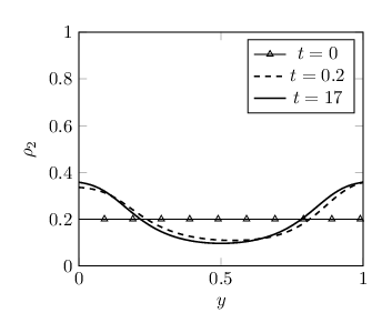
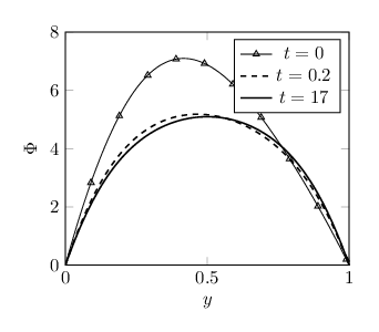
For the first example, the boundary conditions for the electric potential are supposed to be in equilibrium, i.e. for . The dynamics of the particle densities and the electric potential are shown in Figure 1. The solution at time is essentially stationary and, in fact, in equilibrium. Because of the choice of the parameters, the stationary solution is symmetric around .


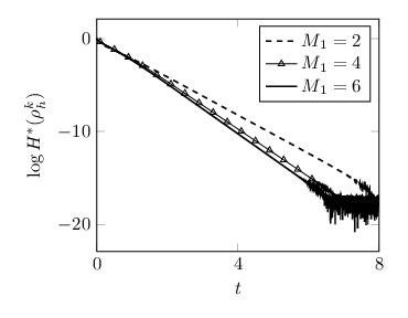
The situation changes drastically when the molar masses are different (example 2). Figure 2 shows the stationary solutions with the same parameters as in the previous example except . Here, the discrete relative entropy is defined by
where is the finite-element solution at time and is the stationary solution. The integral and gradients are computed by the trapezoidal and gradient routines of MATLAB. The semi-logarithmic plot of the relative entropy shows that the entropy converges to zero exponentially fast.


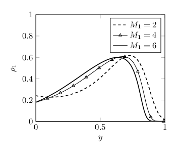
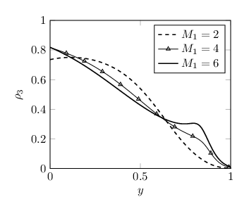
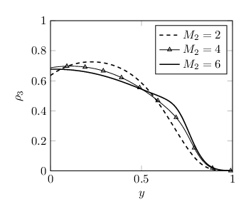
For example 3, we choose the same initial conditions and parameters as before, but we take non-equilibrium boundary data , . The solutions at time for various molar masses are displayed in Figure 3. Since and have both positive charge and the potential on the left boundary is positive, both species avoid the left boundary and move to the right.
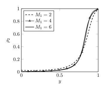
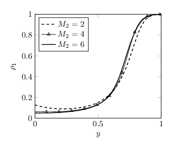
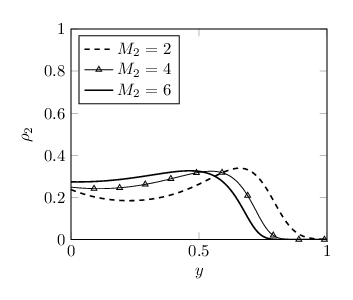
In example 4, we interchange the roles of and , i.e., we choose and . We observe in Figure 4 that the first species is more concentrated at the right boundary while in the previous example, this holds true for the second species.
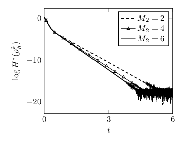
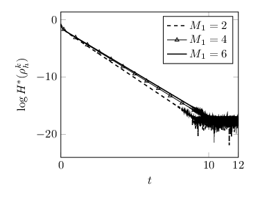
The previous examples show that the convergence rate to equilibrium strongly depends on the ratio of the molar masses. It turns out that this effect is triggered by the drift term, and without electric field, the convergence rates are similar for different molar masses. This behavior can be observed in Figure 5 (example 5), where we have taken the same parameters as in the previous example but neglect the electric field. In this situation, the steady state is constant in space and explicitly computable; indeed, we have . Note that the steady state in the previous examples is not constant.
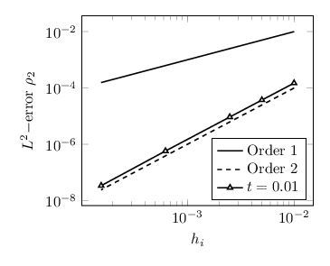
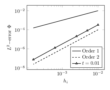
Finally, we compute the numerical convergence rate when the grid size tends to zero for the situation of example 3 (non-equilibrium boundary conditions for the potential). We choose the time and the time step size . The solutions are computed on nested meshes with grid sizes and compared to the reference solution, computed on a very fine mesh with 25601 elements (). As expected, we observe a second-order convergence in space; see Figure 6.


References
- [1] D. Bothe. On the Maxwell-Stefan equations to multicomponent diffusion. In: J. Escher et al. (eds). Parabolic Problems. Progress in Nonlinear Differential Equations and their Applications, pp. 81-93. Springer, Basel, 2011.
- [2] D. Bothe and W. Dreyer. Continuum thermodynamics of chemically reacting fluid mixtures. Acta Mech. 226 (2015), 1757–1805.
- [3] L. Boudin, B. Grec, and F. Salvarani. A mathematical and numerical analysis of the Maxwell–Stefan diffusion equations. Discrete Cont. Dyn. Sys. B 17 (2012), 1427-1440.
- [4] L. Boudin, B. Grec, M. Pavić, and F. Salvarani. Diffusion asymptotics of a kinetic model for gaseous mixtures. Kinetic Related Models 6 (2013), 137-157.
- [5] B. Carnes and G. Carey. Local boundary value problems for the error in FE approximation of non-linear diffusion systems. Intern. J. Numer. Meth. Engrg. 73 (2008), 665-684.
- [6] X. Chen and A. Jüngel. Analysis of an incompressible Navier–Stokes–Maxwell–Stefan system. Commun. Math. Phys. 340 (2015), 471–497
- [7] E. Daus, A. Jüngel, and B.-Q. Tang. Exponential time decay of solutions to reaction-cross-diffusion systems of Maxwell–Stefan type. Submitted for publication, 2018. arXiv:1802.10274.
- [8] K. Dieter-Kisling, H. Marschall, and D. Bothe. Numerical method for coupled interfacial surfactant transport on dynamic surface meshes of general topology. Computers & Fluids 109 (2015), 168-184.
- [9] M. Dreher and A. Jüngel. Compact families of piecewise constant functions in . Nonlin. Anal. 75 (2012), 3072-3077.
- [10] W. Dreyer, P.-E. Druet, P. Gajewski, and C. Guhlke. Analysis of improved Nernst-Planck-Poisson models of compressible isothermal electrolytes. Part I: Derivation of the model and survey of the results. WIAS Berlin, Germany, preprint no. 2395, 2017.
- [11] W. Dreyer, C. Guhlke, and R. Müller. Overcoming the shortcomings of the Nernst-Planck-Poisson model. Phys. Chem. Chem. Phys. 15 (2013), 7075-7086.
- [12] J. Duncan and H. Toor. An experimental study of three component gas diffusion. AIChE J. 8 (1962), 38-41.
- [13] V. Galkin and N. Makashev. Modification of the first approximation of the Chapman-Enskog method for a gas mixture. Fluid Dynam. 27 (1993), 590-596. Translated from em Izv. Ross. Akad. Nauk Mekh. Zhidk. Gaza 4 (1992), 178-185 (Russian).
- [14] J. Geiser. Iterative solvers for the Maxwell-Stefan diffusion equations: Methods and applications in plasma and particle transport. Cogent Math. 2 (2015), 1092913, 16 pages.
- [15] V. Giovangigli. Multicomponent Flow Modeling. Birkhäuser, Basel, 1999.
- [16] V. Giovangigli and M. Massot. The local Cauchy problem for multicomponent flows in full vibrational non-equilibrium. Math. Meth. Appl. Sci. 21 (1998), 1415-1439.
- [17] V. Giovangigli and M. Massot. Asymptotic stability of equilibrium states for multicomponent reactive flows. Math. Models Meth. Appl. Sci. 8 (1998), 251-297.
- [18] M. Herberg, M. Meyries, J. Prüss, and M. Wilke. Reaction-diffusion systems of Maxwell–Stefan type with reversible mass-action kinetics. Nonlin. Anal. 159 (2017), 264–284.
- [19] H. Hutridurga and F. Salvarani. Maxwell–Stefan diffusion asymptotics for gas mixtures in non-isothermal setting. Nonlin. Anal. 159 (2017), 285-297.
- [20] H. Hutridurga and F. Salvarani. Existence and uniqueness analysis of a non-isothermal cross-diffusion system of Maxwell-Stefan type. Appl. Math. Lett. 75 (2018), 108-113.
- [21] A. Jüngel and I. Stelzer. Existence analysis of Maxwell-Stefan systems for multicomponent mixtures. SIAM J. Math. Anal. 45 (2013), 2421-2440.
- [22] E. Leonardia and C. Angeli. On the Maxwell–Stefan approach to diffusion: a general resolution in the transient regime for one-dimensional systems. J. Phys. Chem. B 114 (2010), 151-164.
- [23] J.-P. Loos, P. Verheijen, and J. Moulin. Numerical simulation of the generalized Maxwell–Stefan model for multicomponent diffusion in microporous sorbents. Collect. Czech. Chem. Commun. 57 (1992), 687-697.
- [24] M. Marion and R. Temam. Global existence for fully nonlinear reaction-diffusion systems describing multicomponent reactive flows. J. Math. Pures Appl. 104 (2015), 102-138.
- [25] C. Maxwell. On the dynamical theory of gases. Phil. Trans. Roy. Soc. London 157 (1866), 49-88.
- [26] M. McLeod and Y. Bourgault. Mixed finite element methods for addressing multi-species diffusion using the Maxwell-Stefan equations. Comput. Meth. Appl. Mech. Engrg. 279 (2014), 515-535.
- [27] W. Nernst. Die elektromotorische Wirksamkeit der Ionen. Z. Physikalische Chemie 4 (1889), 129-181.
- [28] K. Peerenboom, J. van Dijk, J. Boonkkamp, L. Liu, W. Goedheer, and J. van der Mullen. Mass conservative finite volume discretization of the continuity equations in multi-component mixtures. J. Comput. Phys. 230 (2011), 3525-3537.
- [29] M. Planck. Über die Potentialdifferenz zwischen zwei verdünnten Lösungen binärer Electrolyte. Annalen der Physik 276 (1890), 561-576.
- [30] S. Psaltis and T. Farrell. Comparing charge transport predictions for a ternary electrolyte using the Maxwell–Stefan and Nernst–Planck equations. J. Electrochem. Soc. 158 (2011), A33-A42.
- [31] F. Salvarani and J. Soares. On the relaxation of the Maxwell–Stefan system to linear diffusion. Submitted for publication, 2018. hal-01791067.
- [32] J. Stefan. Über das Gleichgewicht und Bewegung, insbesondere die Diffusion von Gasgemengen. Sitzungsberichte Kaiserl. Akad. Wiss. Wien 63 (1871), 63-124.
- [33] J. Wesselingh and R. Krishna. Mass Transfer in Multicomponent Mixtures. Delft University Press, Delft, 2000.