Evaluation of Neural Networks for Image Recognition Applications: Designing a - MILP Model of a CNN to create adversarials
Abstract
Image Recognition is a central task in computer vision with applications ranging across search, robotics, self-driving cars and many others.
There are three purposes of this document:
- 1.
We follow up on (Fischetti & Jo, December, 2017) and show how standard convolutional neural network can be optimized to a more sophisticated capsule architecture.
- 2.
We introduce a MILP model based on CNN to create adversarials.
- 3.
We compare and evaluate each network for image recognition tasks.
Keywords:
DNN, CNN, CapsulesGeneral knowledge is based on (Goodfellow et al., 2016).
1 Deep Neural Networks
In the following we will model a neural network in terms of a - Mixed Integer Linear Program (MILP), not for training purposes, but to model well-suited instances for the network. On the contrary we can use the MILP to construct adversarial examples.
This chapter widely cites (Fischetti & Jo, December, 2017).
1.1 Designing a MILP of DNN
1.1.1 Notation
Let a Deep Neural Network (DNN) consist of layers, where marks the input layer and identifies the output layer. Each layer possesses units (or neurons) and pinpoints the unit in layer for all .
We assume a layered, fully connected network i.e. for all and the unit has input edges.
Each layer is connected to the next layer with directed edges, concretely, for there exists an edge that connects directly to for all , for all and .
The DNN can be modelled as a graph :
Let be the finite set of units in the DNN.
Let
be the set of edges in the fully connected DNN.
Let be a given weight matrix. Each weight is assigned to an edge . We define the weight to be the weight between and , which means to be the weight of . We can associate to be the real-valued weights on all edges between layer and .
Let be given bias inputs for all units with and . Note that .
can be modelled as a directed acyclic graph, which means that for any layer there exists no edge for all and .
Let be the output vector of layer and the output value of .
Clearly is the input and the output of .
For every layer the output of this layer can be calculated as follows:
| (1) |
with the output of the previous layer being multiplied with the given weight matrix , a given bias term being added and this sum being fed into a pre-defined activation function .
There are several activation functions, which can be chosen from depending on the specific problem at hand. The activation function e.g. can make negative inputs to zero (like the ReLU function) or e.g. output a probability scale (like the sigmoid function). A non-linear activation function introduces non-linearity to a DNN, encouraging it to learn more complex functions. We set the activation function to be
| (2) |
ReLU is a popular choice, since it is a cheaply performed operation.
Our goal is to create a MILP that modern solvers can solve - this involves not optimizing weight parameters for training, but a model which optimizes the input for given weight parameters, such that this input is the best classifiable instance. On the contrary this allows the construction of adversarial examples.
We need to model accordingly. From (1) we have
| (3) |
in which ReLU is performed on every component of . To this end, we can write the linear conditions
| (4) | ||||
to separate the positive and the negative part.
If , we choose thus leading to and (the range of is defined in (4)).
If , we choose thus leading to and . Due to (3), this implicates , which reflects the ReLU property for negative input.
The above solution and is not unique, since and are also solutions for any positive and . To achieve uniqueness, we must find a solution in which does not apply.
One may think to minimize , but this would implicate an undesired minimisation of the ReLU-function. One may also think to introduce as a non-linear constraint to achieve that either or will be , however this would contradict the MILP approach of having just linear constraints.
We solve this by introducing an activation variable to the model:
| (5) | ||||
| (6) | ||||
| (7) | ||||
where are pre-calculated bounds such that is valid for all . These bounds are calculated by a MILP solver.
Conditions (5) - (7) is equivalent to
If , then , which means that the corresponding unit in is not activated. This would encourage a trivial solution of , however this is undesirable, because our goal is to find well constructed instance that are correctly classified. Consequently, we penalize the instance of in the cost function to avoid a trivial solution. Incorporating the binary variable into the objective function qualifies our model as a - Mixed Integer Linear Program.
In order for modern solvers to solve a MILP efficiently, we introduce upper- and lower bounds for and :
| (8) | ||||
| (9) |
One way of calculating tight upper bounds is to step through all units and for every we delete all constraints and variables associated with any other unit in either the same layer or in any higher layer, and then we solve the model (10)-(12) in one round to maximize and in a second round to maximize . This gives a far more accurate tight upper bounds for each units output and accelerates MILP solvers.
Putting all pieces together delivers the following - MILP model as presented by (Fischetti & Jo, December, 2017):
| (10) |
| (11) |
| (12) |
This model formulation is feasible, since for any fixed input i.e. , every is uniquely defined by (3).
We seek minimal unit activation values in a matter such that is a well constructed example.
Surely for all and for all is a solution, but trivially superfluous. To avoid such superfluous solution to be optimal, we set into the cost function, so that any unit with activation value will be penalized. We seek to be as often as possible i.e. we penalize the occasion . Even though the parameters for can be negative, it is only logical for a DNN to have a non-negative output. As said before, applying encourages a trivial solution for (namely ), so we can set each to a chosen non-negative value in accordance of how greatly we want to penalize the possibility of the trivial solution problem occuring.
Furthermore, we can set .
In this way, there are no specific units or layers of that are penalized sharper or milder.
1.2 Creating adversarial examples
The described model however is not suited for training. In a DNN we have weight parameters and to be optimized, but these are fixed in . We do not have any training involved in the model. Instead, is designed to implicitly compute the best possible input example , that can best be classified by the network.
Inversely, we can modify to compute input examples that are worst possibly classified by the network. This will result in slightly different inputs, called adversarial examples, that the DNN will missclassify upon.
One application is the MNIST dataset consisting of hand-written digits as image instances.
If an image of a digit is classified correctly as , the goal of is to find a similar image which is classified as , with . As (Fischetti & Jo, December, 2017) proposes, we can set , so the adversarial image of a should have label .
Say we want the activation of the required wrong digit in layer to be at least larger than any other activation, we get
| (13) |
One can also think of modifying the cost function accordingly
| (14) |
with as negative cost: we can encourage the activation of the required wrong digit . Conceivably, we can further penalize high activations of the other units with positive costs.
For the adversarial to be as similar as possible to , we change every image pixel, such that the difference between them is close to :
| (15) | ||||
| (16) | ||||
| (17) | ||||
| (18) |
Adding (13) and (18) to modifies the model to construct adversarials :
| (19) | ||||
| (20) |
| (21) |
| (22) |
| (23) |
| (24) |
The additional constraint for all guarantees that no pixel is changed by more than 0.2, thus leading to more pixels to be changed in total.
The resulting adversarial images for the MNIST dataset are presented in Figure (1) and represent a first approach to building adversarials for DNNs with MILP models.

1.3 DNN Training
The general idea of DNNs in the context of supervised learning is to feed input data into the DNN, perform a forward pass, calculate the error between the output value and the desired target value, and then update the weights using the backpropagation algorithm in order to minimize the error. By doing this iteratively many times the DNN will "learn" its weights to match the output values with the desired target values.
A DNNs trainable parameters are its weights and biases . For training, each layer with corresponding input weights must be initialised, e.g. the (He et al., February, 2015) initialisation draws values from a Gaussian distribution centered at 0 with standard deviation = , where is the number of units of the previous layer.
We define the loss function as the mean squared difference of the total error:
with equals the number of instances. The desired target activation of of the instance is defined by . The activation value of , namely , for the instance is computed by (3).
Depending on the specific problem at hand, there are different loss functions (Janocha & Czarnecki, February, 2017).
A forward pass is given when applying (3) to every unit in the DNN.
Using the back-propagation algorithm (Lecun et al., 1989), we can calculate how much a slight shift of an individual weight parameter affects the total error. Therefore, we calculate the derivative of E in respect to and solve this with the following chain rule (Avrutskiy, December, 2017)
| (25) | ||||
| (26) | ||||
Using a gradient descent method, all can be updated repeatedly by taking a step in the direction of steepest decrease of towards its minimum. For the sake of simplicity, we introduce batch gradient descent (Ruder, June, 2017):
| (27) |
where represents a small fixed learning rate and needs to be chosen carefully. If is too small, gradient descent works too slowly; if is too large, gradient descent may overshoot the minimum and may fail to converge (Karpathy & Johnson, Spring, 2018).
Batch gradient descent steps through all instances of the training set, calculates the full loss function over the entire data set, and then performs one round of weight updates (Karpathy & Johnson, Spring, 2018). In practice the training data can have millions of instances, therefore it seems wasteful to use batch gradient descent, because training would be too slow (Karpathy & Johnson, Spring, 2018). Batch gradient descent has its advantages (Karpathy & Johnson, Spring, 2018), but more commonly other optimizers are used for more efficiency (Ruder, June, 2017). Adaptive Moment Estimation (Adam) is widely used as gradient descent optimizer, as it adaptively computes the learning rate, thus sparing the need of finding an efficient learning rate experimentally (Ruder, June, 2017).
Repeating (27) iteratively, until E reaches its global minimum, is the process of DNN training. Local minima and sattle points are to be avoided (Dauphin et al., June, 2014).
1.4 Evaluation
As (Fischetti & Jo, December, 2017) shows, it is possible to use MILP models of DNNs to satisfyingly construct adversarial examples. The MILP approach, if at all, is not suited for finding optimal weight parameters.
We will see why DNNs are not efficient for image applications and follow up on the current state-of-the-art in image classification: Convolutional Neural Networks.
2 Convolutional Neural Networks
2.1 Introduction
In the following, we will follow up on how Convolutional Neural Networks work, access them mathematically and finally introduce a first approach of a MILP model to create adversarial examples.
It turns out that standard neural nets are inefficient in practise for image classification. One of the main reasons for this are:
- 1.
They perform weakly with highly invariant data such as different positions of the objects in the image (Karpathy & Johnson, Spring, 2018) (see figure (2)).

Figure 2: (Kaggle, 2014)
A DNN, which is trained with the dog in the first image, does not recognize the dog in the other images, because it is not able to learn translational invariance. It would have to learn all of these images to recognize the same dog at different positions. - 2.
There are extensively large amounts of network parameters to calculate e.g. an image in colour of more respectable size, e.g. 200x200x3, would mean that each neuron in the following hidden layer has weight parameters. Such great numbers of parameters increases the risk of overfitting (Karpathy & Johnson, Spring, 2018).
Convolutional neural networks (CNNs) have proven to be the current state-of-the-art architecture for classifying images using deep learning (Wikipedia, 2018c). CNNs have the desirable property of being able to detect objects, even though they might be invariantly shifted (Wikipedia, 2018c).
The best so far performance marked on the MNIST database scores an error rate of (Wikipedia, 2018d), using complex CNNs and preprocessing measures.
We reflect more detailedly on how CNNs work in the following. Our goal is to introduce a mathematical approach on constructing adversarials with a MILP.
CNNs take advantage of image data provided in 3 dimensions: width, height and depth (number of colour channels). Concretely, CNNs consist of a sequence of layers, namely Convolutional Layer, ReLu, Pooling Layer and Fully-Connected Layer (Karpathy & Johnson, Spring, 2018).
These layers are stacked upon eachother, forming the CNN’s architecture. We will see how a basic CNN architecture looks like.
2.2 Architecture
2.2.1 Input layer
We define the input images as for the height dimension , the width dimension and the depth dimension , where is the number of input maps (not to be confused with batch size). We assume that the next layer is convolutional (identified by superscript in paragraph (2.2.2) . We think of the input images as tensors:
| (28) | ||||
| (29) | ||||
| (30) |
Let define the pixel integer value in the height, the width and the depth of the input image. For RGB colour images, we have . For these colour maps, each is a tensor with integer values between , because each colour map displays its colour array as an -Bit integer (Goodfellow et al., 2016). Even though this document treats image applications i.e. , we will keep the depth dimension generic.
2.2.2 Convolutional layer
Intuition
The convolutional layer is the core element of a CNN. They consists of pre-initialised convolutional kernels of square size that perform linear combinations of pixel values (Wikipedia, 2018c).
Applying convolutional operations to an image is the biological simulation of how the human eye works. The human visual cortex incorporates receptive fields, a cluster of neurons that result in one firing neuron. The receptive field helps the retina to identify objects in their shape and colour, adjust sharpness of vision and reduce the flood of incoming information so that signals can be processed more easily (Wikipedia, 2018a). Convolutional kernels imitate properties of the receptive field.
The idea is that a kernel with certain components is able to detect a certain figure in the image. According to the given components of the kernel, the kernel is able to recognize the presence of a specific figure, edge or characteristic in the image. The more accurate these components of the kernel are, the more precise it can spot that specific figure. These components can be trained, making the components the weight parameters of this layer.
A kernel is an operator performing dot multiplications along the pixel values according to its kernel compontents, the result is a real value (figure (4)). Then the kernel moves one stride further to perform the next operation. Effectively, the kernel slides through the input maps with a certain stride length (Karpathy & Johnson, Spring, 2018), layer by layer, over the entire width and height of the input volume, while at each position an operation is executed. This is performed on all depth maps.
For instance, on the left hand side figure (3) shows an image of two different coloured boxes. This kernel e.g. measures the differences between the borders of the two squares:

Suppose the image is given in pixel values as in (28). The kernel given above will calculate the pixel differences at each pixel cluster - the red dot clusters have disparate differences, as do all other clusters at the borders. The kernel outputs an integer for each border cluster and zero for all other clusters. The right hand figure (3) shows the output when applying this kernel. Only vertical lines are highlighted. This illustrates how this kernel works as an receptive field in order to identify vertical lines.
We can apply further different kernels to detect horizontal lines, edges, angles etc. The task of CNNs is to learn the values of all given kernels, such that each kernel is able to identify a certain figure in the image. Multiple convolutional layers give higher level convolutional kernels that are able to detect more comlex shapes and sophisticated figures (Karpathy & Johnson, Spring, 2018). The further we move up in layers, the more complex and higher level the extracted features detected by kernels get.
Since each kernel is moving across the input tensors, it is sharing its weights with many input units. This makes CNN predestined to image recognition, since it reduces the amount of computation significantly. Importantly, convolutional kernels enable already learned data to be shared across space, meaning they enable translational invariance of the input data, such as figure (2): recognizing the dog in every corner of the image, even though only one of them has been trained upon.
Notation
Let be the number of convolutional layers in the CNN, where is a hyperparameter to the CNNs architecture. For each convolutional layer there exist kernels, where is also a hyperparameter. Let pinpoint the kernel in convolutional layer for all . For all and we define to be a tensor with square size :
| (31) |
where marks the row and column component of kernel with and . Note that is a hyperparameter and needs to be chosen for each layer .11
1
and must hold; we assume that the kernel size is significantly smaller than the input size, since we want to have small clusters in order to accurately find small figures, lines, edges etc.
Suppose that denotes the input of a convolutional layer and are the input maps, where is the number of input maps of .
Similarly, suppose that denotes the output of a convolutional layer and are the output maps. There are output maps of layer .
As (Zhang, 2016) suggests, one can initialize the kernels with random values drawn from a uniform distribution
where denotes a uniform distribution with upper and lower bounds of . Bias values can also be taken into account here, however we will omit these for the sake of simplicity. Each kernel can be associated with a certain form in the image that it can analyse. Therefore it is advisable to add many different convolutional filters to the layer to achieve high accuracy of identifying details (Zhang, 2016).
The convolutional operations for every layer are performed as follows:
| (32) | ||||
| (33) | ||||
| (34) | ||||
| (35) | ||||
| (36) | ||||
| (37) | ||||
| (38) | ||||
| (39) | ||||
| (40) | ||||
| (41) | ||||
where is the stride step to which the kernel iterates through the rows and columns of and is the number of zero-paddings. The kernel slides through the rows and colums in steps of ; note that each layer has a fixed stride , such that applies to all kernels . Clearly must always be valid, otherwise the kernels would not overlap with the maps, thus losing information. Applying strides reduces the size of the output maps.
Zero-padding is the number of additional frames that are applied to , such that a left vertical vector of zeros, a right vertical vector of zeros, a top horizontal vector of zeros and a bottom horizontal vector of zeros are appended to tensor . This hyperparameter can be used to control the output map size.
Furthermore, it becomes evident that certain strides are not valid, since needs to be an integer number22
2
same for height respectively. so that convolutions on only whole pixels are provided. Concretely, the constraint
| (42) |
needs to be given for a valid stride . If (42) is not valid for a fixed , then we can see for which the constraint
| (43) |
becomes valid. It is important that these constraints must simultaneously hold for each dimension2. Note that
| (44) |
needs to be fulfilled in order for the size of the output maps not to become larger - this would add redundancy with many zero pads thus increasing computation. High level machine learning libraries are capable to automatically adjust (43) by adding zero-padding or cutting down and to make it fit (Karpathy & Johnson, Spring, 2018).
The calculations (35)-(37)
define the convolutions when the filter slides column for column through the first row. Then the kernel slides column for column through the second row ((38)-(39)).
This continues until the kernel convolutes through the last row ((40)-(41)).
This procedure (35)-(41)
represents how a kernel (32) convolutes entirely over an input map (33) and produces an output map (34) (see figure (4) for illustration). Then the kernel performs the entire convolution upon all next input maps (33), and then the whole procedure is done all over again with the next kernel (32). The result are output maps (34) each of which have size and for all and .

ReLU
The Rectified Linear Unit Layer (ReLU) makes all values of the convoluted image non-negative. It is an activation function defined in (2) on page 2. ReLU is not really a separate layer, but more an operation performed on the previous convolutional layer. Commonly it will be performed right after the convolutional layer and therefore counts as part of the convolutional layer (Goodfellow et al., 2016).

Let
| (45) |
be the output maps of a convolutional layer and its corresponding hyperparameters, as defined in (35) - (41).
We will use the notation of (11) on page 11 to model ReLU:
| (46) | ||||
| (47) | ||||
| (48) |
Concretely, we introduce an activation variable for every unit of map , for every map and every convolutional layer . Similar to (4) on page 4, the activation value equals if the associated is negative, thus turning the associated into . Else, if the associated is positive, the activation value is , thus legitimizing the associated to be .
2.2.3 Pooling layer
The function of pooling layers in a CNN architecture, is to down-size the input maps in order to reduce the amount of parameters to avoid overfitting and reduce computation (Goodfellow et al., 2016).
Pooling is similar to a kernel: it is an operation that takes pixel clusters of the input maps and combines it to one single pixel in the next layer, as can be seen in figure (6). Unlike convolutional kernels, pooling kernels do not have any component values.
There are several pooling functions, we will focus on max pooling as it is commonly used. Max pooling will take the maximum value of a kernel-sized pixel cluster and project it onto the output tensor. These maximum pixel values represent the most dominant and evident shapes in the original input map, only they are passed along and the rest of the pixel information is disregarded (Karpathy & Johnson, Spring, 2018).

Notation
Let be the number of max pooling layers in the CNN. Each max pooling layer consists of one max pooling kernel of which each has a predefined squared size . Note that is a hyperparameter and needs to be chosen for each layer . Commonly , or else too much information is lost (Karpathy & Johnson, Spring, 2018).
Suppose that denotes the input of a pooling layer and are the input maps, where is the number of input maps of . Let have size for all and .
We can model a max pooling layer as follows:
| (49) | ||||
| (50) | ||||
| (51) | ||||
| (52) | ||||
| (53) | ||||
| (54) | ||||
| (55) | ||||
| (56) | ||||
where defines the specified stride length of each max pooling layer . For each stride, must be valid for all , otherwise input pixels are skipped (Karpathy & Johnson, Spring, 2018). The stride needs to be chosen in a way that33 3 same for height respectively.
| (57) |
is integer, in other words such that
| (58) |
Given a , we are given the input map (49), on which we apply the max pooling kernel at the first row through all columns (50)-(52) and storing the max value of each -pixel cluster of as a single value . Then max pooling is performed at the second row through all columns (53)-(54). and the max values are stored in . This continues for all rows, until finally max pooling is done on the last row through all columns (55)-(56)
with the corresponding max values stored in . This whole procedure is done for all input maps (49).
The result of a max pooling layer are output maps , each of which have size and for all .
Modelling max pooling in a way that it can be used by modern MILP solvers, requires the use of binary activation variables e.g. given the first max pooling operation (50), we can transform it into:
| (59) | ||||
| (60) | ||||
| (61) | ||||
| (62) | ||||
| (63) | ||||
| (64) |
For this first max pooling kernel, we assign times activation variables . They correspond to the first pixel cluster of the input map - only one of them will be the maximum value (59), thus having activation value , while the rest have . The maximum value will satisfy (60) for all (63). Specifically is equals to the maxium, as to which the activation variable triggers (61) - the remaining activation variables equal (62). This works for every input map (64) and every max pooling layer (64).
2.2.4 Fully-Connected layer
All the pixel representations of the last layer (either convolutional or pooling) are reshaped into one long unit layer - the so called flattend layer (Wikipedia, 2018c). Then each unit of the flattend layer connects entirely to the fully-connected layer. Unlike a convolutional layer, the units in the fully-connected layer do not share weights ((Karpathy & Johnson, Spring, 2018)).
Notation
Let be the output of the last convolutional or pooling layer of the CNN. Suppose is the size of each with . Define
| (65) |
for all , and . This gives a flattend layer of size and represents merely a reshape of the pixel maps into a single long unit layer.
Let the next layer be the fully-connected layer with size , where is the number of units of the fully-connected layer. Since we are one layer behind the output class layer, it is advisable to choose , we want to decrease the units to get closer to the number of units in our output class layer. The flattend layer is fully-connected with the fully-connected layer i.e. there are trainable weight parameters on each edge connecting each flattend layer unit with every fully-connected layer unit. Set to associate the weights on all edges between and , concretely is the weight between unit of the flattend layer and unit of the fully-connected layer. The value of a fixed unit of is calculated by
| (66) |
we choose ReLU to be the activation function for .
2.2.5 Output layer
The output class layer is the final layer of the CNN and corresponds to the classification of the input image, where is the number of classes of the CNN. This layer is fully-connected to , i.e. we associate all weights between layer and as weight matrix . The value of a fixed unit of is calculated by
| (67) |
where softmax (Wikipedia, 2018e) is defined by
| (68) | ||||
| (69) |
Each entry is a value between and all entries add up to . Applying softmax as activation function to allows the entries to be activation values, thus allows to interpret the activation of the output class layer as probability predictions of each class.
This part of the CNN is similar to a standard neural network and every methode and technique, which applies to standard vanilla neural nets, can also be applied to this part e.g. softmax as activation, dropout measures etc (Karpathy & Johnson, Spring, 2018). Each output neuron will give a prediction in form of a probability as to whether this object class is recognized in the image. The highest probability (closest to 1) will be the total prediction for the image (Wikipedia, 2018c).
2.3 CNN training
Choosing a CNNs layers and hyperparameters remains an uncertainty, commonly however there are rules of thumb to the hyperparameters (Karpathy & Johnson, Spring, 2018). A basic sequence of CNN layers can be seen in figure (7).

A CNN can hold several convolutional and max pooling layers, which alternate, as in figure (8) This way, a CNN can be build to a much deeper architecture and hopes are that performance will be more accurate - not necessarily though due to overfitting and many more options to tweak (Brownlee, September, 2016).

Similarily to DNNs, the values of the convolutional filters as well as the weight matrices of the fully-connected layer are trainable paramaters for CNNs. We use backpropagation and gradient descent to improve each of the filters weights (Zhang, 2016) (1.3). Cross-entropy as loss function is commonly used (Karpathy & Johnson, Spring, 2018).
2.4 MILP formulation for a CNN
Analogeously to designing a - MILP formulation for DNNs (10)-(12), we can formulate a - MILP representation for CNNs.
We set several assumptions:
- •
The CNN consists of layers and each is is a block: a convolutional layer (including ReLU) is followed rigidly by a max pooling layer i.e. the input of is the output of the max pooling layer of block and the output of is the input of the convolutional layer of block . This allows the MILP to be written in an iterative structure.
The consequence is we have hyperparameters where superscript points that this pooling layer is part of block . Note that for this MILP. The MILP is customizable to allow a more dynamic use of alternating layers. - •
The flattend layer , the fully-connected layer and the output class layer are not part of a block and are defined separately. The flattend layer follows after the last block .
- •
For the sake of simplicity, bias units are omitted.
- •
- •
It is problematic, that the use of the non-linear softmax activation function cannot be used in a MILP model. Due to the unchanged derivative the linear approximation does not work either. This also rules out the sigmoid function as a possible alternative. This is why we will use ReLU in the output class layer as activation.
- •
Every convolutional kernel value for all , and all blocks are given values.
- •
The weight parameters and for all , and for the fully-connected layer and the output class layer respectively are given values.
- •
Hyperparameters to set:
- –
The number of blocks consisting of a convolutional layer, ReLU activation and max pooling.
- –
The size of the input images.
- –
The number of input channels .
- –
The number of convolutional kernels for each block .
- –
The size of the convolutional kernels for each block .
- –
The size of the convolutional stride for each block .
- –
The number of convolutional zero-padding for each block .
- –
The size of max pooling kernel for each block .
- –
The size of the max pooling stride for each block .
- –
The number of units in the fully-connected layer .
- –
The number of classes in the output class layer.
- –
| substitutions: | ||||
| (70) | ||||
| (71) | ||||
| (72) | ||||
| (73) |
| (74) | ||||
| (75) | ||||
| (76) | ||||
| (77) | ||||
| (78) | ||||
| (79) | ||||
| (80) | ||||
| (81) | ||||
| (82) | ||||
| (83) | ||||
| (84) | ||||
| (85) | ||||
| (86) | ||||
| (87) | ||||
| (88) | ||||
| (89) | ||||
| (90) | ||||
| (91) | ||||
| (92) | ||||
| (93) | ||||
| (94) | ||||
| (95) | ||||
| (96) | ||||
| (97) | ||||
| (98) | ||||
| (99) | ||||
| (100) | ||||
| (101) | ||||
| (102) | ||||
| (103) | ||||
| (104) | ||||
| (105) | ||||
| (106) | ||||
| (107) | ||||
| (108) | ||||
| (109) | ||||
| (110) | ||||
| (111) | ||||
| (112) | ||||
| (113) | ||||
| (114) | ||||
| (115) | ||||
| (116) | ||||
| (117) | ||||
| (118) | ||||
| (119) | ||||
| (120) | ||||
| (121) | ||||
| (122) | ||||
| (123) | ||||
| (124) |
This MILP formulation is feasible, since for any fixed input i.e. , every other unit in the system is uniquely defined by (81)-(101).
2.4.1 Explanation
This MILP model is designed to be a minimization problem (74)-80), in which the value of each unit in every layer is minimized.
Explanation of (74): as mentioned, this MILP is a minimization problem. The variables are mixed i.e. they are real or binary integers. The objective function and the constraints must be linear. All variables of blocks must be minimized, as well as all pixel values of each map, , of all input maps . The CNN’s input maps are marked as , the size is . The cost parameters can be set as for all , , and (110)-(113).
Explanation of (75): the units in represent the convoluted units. The number of maps make up the number of input maps times the number of kernels used. The size of these maps have changed depending on the kernel size, the stride and the padding. The cost parameters can be set as for all , , and (115)-(117).
Explanation of (76): the convoluted maps are fed through the ReLU function, which gives us the unit maps , the size is unchanged. The cost parameters can be set as for all , , and (115)-(117).
Explanation of (77): the binary variable corresponds as an activation variable used for the ReLU function. We penalize the occurrence of , we may initialize the cost parameters in a way in which how much we want to penalize this occurrence, possibly between .
Explanation of (78): this minimizes the binary activation variable used for max pooling. For each pooling kernel (118) in an input map , we need to associate each entry (119)-(120) with this - activation variable. We may set the cost parameters e.g. .
Explanation of (79): the units in represent the fully-connected layer . We can choose the cost parameters to be . Furthermore stands for the activation variable used for ReLU in the fully-connected layer. Similar to and , we can choose the cost parameters depending on how much we want to penalize the activation.
Explanation of (81): the input maps to block are convoluted. The unit values are multiplied by a kernel value and all kernel values are summed up. This convolution depends on the kernel size (114), the stride and padding measures. A kernel moves along the an input map horizontally, then vertically, and then performs this on all input maps , before the next kernel (121) repeats this procedure. As a result we have with changed size.
Explanation of (82): by introducing variable , we can tackle a non-linear activation function to fit into a MILP. For this we introduce an activation variable . The purpose of (83)-(86) matches the thoughts of (5)-(7).
Explanation of (87): we define an activation variable (90) for each input map , we have pooling kernels and each kernel has (122) components. We need to step through each component and guarantee that each kernel only activates one (87). This activation identifies the max value of the pixel cluster in maps (88)-(89).
The constraints (81)-(90) characterize the convolution-, the ReLU and the max pooling layers in a block . The last block will give us maps for all (119) and (120). We use these maps and flatten them out, row by row, map by map, into the flattend layer (91).
Explanation of (92): we then construct the fully-connected layer . Every component of (123) is a linear combination of each flattend layer component together with a connecting weight. Every component of the flattend layer is connected with every component of the fully-connected layer with corresponding weight parameters . Note that the size of the maps is unchanged from the last block. For ReLU activation, we introduce variable (93) and binary activation variable (94). For (95)-(96) we proceed in similar terms to (85)-(86).
Explanation of (97): finally we introduce the output class layer with classes (124), whose weights are fully connected to the previous fully-connected layer. As pointed out in the assumptions, we cannot use sigmoid or softmax as activation functions, but we know how to construct ReLU as linear constraint for this MILP: (98)-(101) is an identical approach to the ReLU activation above.
Explanation of (102)-(109): similar to (12), we introduce upper- and lower bounds for each unit in order for modern MILP solvers to work more efficiently:
| (125) | ||||
| (126) | ||||
| (127) | ||||
| (128) | ||||
| (129) | ||||
| (130) | ||||
| (131) | ||||
| (132) | ||||
| (133) | ||||
| (134) | ||||
| (135) | ||||
| (136) | ||||
| (137) | ||||
| (138) | ||||
| (139) | ||||
| (140) |
One way of calculating tight upper bounds is to step through all units: we fix a unit and delete all constraints and variables associated with any other unit in either the same layer or in any higher layer, and then we solve the model (74)-(124) in one round to maximize each unit. This gives as a far more accurate tight upper bounds for each unit’s output and accelerates MILP solvers.
2.5 Creating adversarial examples
The described MILP model in (2.4) however is not suited for training. We have kernel values and weight parameters in the fully-connected layer , to be optimized, but these are fixed initializations in (2.4). We do not have any training elements involved. Instead, the MILP is designed to implicity compute the best possible input example , that can best be classified by the network.
Inversely, we can modify the MILP to compute input examples that are worst possibly classified by the network. This will result in slightly different inputs, called adversarial examples, that the CNN will missclassify upon. This procedure is analogeous to (1.2) where we found adversarials with DNNs. Again, we will take the MNIST dataset to base the MILP upon. If an image of a digit is classified correctly as , the goal of our CNN MILP is to find a similar image which is classified as , with . As already done by (Fischetti & Jo, December, 2017), one way is to set , so the adversarial image of a should have label .
Say we want the activation of the required wrong digit in the output class layer to be at least larger than any other activation, we get
| (141) |
where corresponds to the output class layer units of the adversarial. One can also think of modifying the cost function accordingly
| (142) |
with as negative cost: we can encourage the activation of the required wrong digit . Conceivably, we can further penalize high activations of the other units with positive costs.
For the adversarial to be as similar as possible to , we change every image pixel, such that the difference between them is close to :
| (143) | ||||
| (144) | ||||
| (145) | ||||
| (146) | ||||
| (147) | ||||
| (148) |
An additional constraint for all (146)-(148) guarantees that no pixel is changed by more than 0.2. This means that instead of few significantly changed pixels, instead more pixels are changed in total less significantly.
By adding (142) and (143) to the objective function of the MILP, as well as constraints (144)-(148) and (141) to the MILP, we can construct such an adversarial example .
2.6 Evaluation
Historically CNNs are the most popular form of artificial neural network to perform image application tasks e.g. LeNet- (LeCun et al., 1998) as one of the first CNNs by Yann Lecun (Lecun et al., 1989), deep CNN AlexNet (Krizhevsky, 2009) used for CIFAR dataset classification and first introduced ReLU activation (Karpathy & Johnson, Spring, 2018), or deep CNN ResNet (He et al., December, 2015) using network layers to fit a residual mapping (Karpathy & Johnson, Spring, 2018). For good reason, because they all achieved state-of-the-art accuracy at moderate to affordable computational cost (Karpathy & Johnson, Spring, 2018). They maintain translational invariance and shared weight parameters is more efficient than vanilla DNNs.
Feeding the MILP model (2.4) into a modern MILP solver (CPLEX) to create adversarial examples remains to be done. These may then be compared to the results of the DNN MILP presented by (Fischetti & Jo, December, 2017), in order to arrive at an evaluation which MILP model is more suitable.
3 Capsule Networks
This chapter is widely based on (Hinton et al., 2017) by Geoffrey Hinton.
3.1 Equivariance
With the help of convolutional kernels, CNNs manage to detect objects in images that are translational invariant (2).The convolutional filters move iteratively through all image areas, which makes it possible to translate the same structure detected in one region across the entire image and keep that information stored within its kernel weights. Training a CNN with a center-positioned object, enables the CNN to classify that same object to the left, right, up or down (2). This is why CNNs are robustly resistant to translational invariance (Goodfellow et al., 2016). However, this does not apply for any transformation applied to the object in the image. If the object is rotated, flipped, scaled, deformed, reassembled etc. the CNN fails to classify the object correctly (Hinton et al., 2017). Further training with these transformed objects would be needed and further kernels would be needed to cover all the different transformations. In short: CNN lack equivariance (Hinton et al., 2017). Equivariance is a concept to describe how objects still stay the same, eventhough they are transformed, rotated, in a different light etc. and thus need to be classified as the objects they are, regardless of any transformation (Hinton et al., 2017). This concept matches how human vision works: when an object is viewed, the human eye sets fixation points to process the area of the object at an high resolution while ignoring irrelevant details (Hinton et al., 2017). Furthermore, the brain is capable to understand the instantiation of a transformed object, in order to identify it.
This is the reason and motivation for (Hinton et al., 2017) to introduce a new kind of architecture to classify objects equivariantly - in the following, we follow up on this innovative architecture for computer vision, namely Capsule Networks (CapsNets) (Hinton et al., 2017). CapsNets expand on human vision such that objects are detected as such, regardless of any transformation in the image. Also, in crowded scenes with overlapping elements each element can segmentedly be classified (Hinton et al., 2017).
CapsNets are based on CNNs, replacing max pooling by an routing-by-agreement algorithm (Hinton et al., 2017). Max pooling extracts the major element in a conv map and erases the rest. This causes a lot of information to be lost, moreover it does not serve to achieve equivariance (Hinton et al., 2017). Maintaining translational invariance however in addition to equivariance is certainly desired for CapsNets.

In the following, we discuss the CapsNet architecture presented in (He et al., February, 2015) and our goal is to arrive to an evaluation, comparing CapsNet to state-of-the-art CNNs in image recognition applications.
The dataset on which CapsNet in (Hinton et al., 2017) is based on, is the MNIST dataset ((Wikipedia, 2018d)).
3.2 CapsNet Architecture
3.2.1 Input layer
Let the input be a grey-scaled MNIST image i.e. a tensor of integer values ranging between .
3.2.2 Convolutional layer
The first layer is a standard convolutional layer with included ReLU operation. We maintain convolutional layers for CapsNets, because we want to "replicate learned knowledge across space" (Hinton et al., 2017), thus preserving translational invariance. This first layer of convolutional operations is looking for low level edges and simple curves in the input image. different convolutional kernels are applied, with a stride of and no padding. This gives an output of maps.
Let denote these maps for , and be the value in row and column of the map, , , . ReLU (2) is applied as activation function on all , , . So we have convolutional maps of size consisting of non-negative integers. An additional bias term leads to trainable parameters in this layer (Pechyonkin, February, 2018).
3.2.3 PrimaryCaps layer
So called PrimaryCapsules (Hinton et al., 2017) is a convolutional layer with "primary capsules" of convolutional -D capsules. Concretely, we have 32 multidimensional "kernels" (or primary capsules), each consisting of convolutional kernels and a stride of , that sees the whole input of the maps. The result is -D maps. Basically the input maps are restacked into "decks" with maps each deck. This gives us times stacks, each consisting of -D vector components.
Let be the stacked decks, and be the vector in row and column in the deck, , , . Then the -D vector in is defined by
where represents the convoluted map of .
Each deck is called capsule layer and each component is called capsule. Clearly each capsule layer has 36 capsules. One can think of an capsule as a group of neurons that collectively produce an activity vector with one element for each neuron. On the one hand, vanilla DNNs output a scalar value for each neuron, which illustrates how high the activation of that neuron is, in other words whether a certain entity of an object is present or not (Wikipedia, 2018c). With CapsNets, on the other hand, a capsule outputs an activity vector (Hinton et al., 2017).
Since each of the primary capsules applies eight convolutional kernels to the layer’s input, this leads to trainable parameters in this layer (including a bias term) (Pechyonkin, February, 2018) that are trained by backpropagation.
Activity vector
Computer graphic programs take instantiation parameters of an object as input and then output the rendered image. Inverse rendering implies taking an image and finding out the instantiation parameters of existing objects.
It is the major task of CapsNets to learn instantiation parameters of objects in an image, in order to achieve equivariance (Géron, 2017). An objects instantiation parameters include exact position, size, deformation, rotation degree, velocity, lighting, albedo, hue, texture etc (Géron, 2017).
The instantiation parameters are represented by the orientation of the activity vector of a capsule (Hinton et al., 2017). The length of the activity vector marks the probability that a certain entity exists, analogeous to the activation value of single-scalared DNN neurons (Hinton et al., 2017).
3.2.4 DigitCaps layer
In the following procedure the activity vectors are "squashed" applying a squashing function (Hinton et al., 2017):
| (149) |
The squashing function scales a vector to have length between and , while maintaining the orientation. It ensures that long vectors get shrunk to a length slightly below 1 and short vectors get shrunk to almost zero length (Hinton et al., 2017).
The squashing function (149) introduces non-linearity to the CapsNet and acts as an activation function: since the length of the activity vector represents the probability that an object exists, it is desired to have vector lengths not exceeding and not be inferior to .
We apply the squashing function to all -D capsules; we obtain normalized activity vectors, the orientation stays identical.
Then the -D capsules are reshaped into -D capsules called , with
where notates the squashed capsule of .
Now each capsule is multiplied with an individual weight matrix
| (150) |
with as input capsule and the number of digit classes.
The weight matrix is an affine transformation matrix and stores learnable information about the exact part-whole relationship of each entity of the entire object. It is initialized at the beginning and the values are learned with backprogagation iteratively. Each capsules activity vector stores instantiation parameters of an objects entity and the weight matrix stores data for the exact spatial relationship of the entity regarding the entire object. E.g. if the input image is a face and capsule stores information about the eye, then the weight matrix gives information on how exactly the eye is to be spatially positioned in the face, such that essentially a proper face is detected. In CNNs, such spatial information is not stored, which is why Pablo Picassos famous "Portrait of woman in d‘hermine pass" figure (10) will falsely be classified by CNNs as a face. This makes CNNs vulnerable to adversarial attacks.
The matrices represent a part-whole relationship. This tells us in what manner a lower level entity, a capsule , fits in to with a higher level entity/object. E.g. may store information about a curve, and represents in what posture curves fit into the digit "0", then has significant length; whereas there are no curves in the digit "1", consequently is a short activity vector for that same curve capsule .

"Portrait of woman in d‘hermine pass"(Picasso, 1923)
As in (150), for all every capsule is transformed into via matrix-vector multiplication44 4 This works, since and . with every digit class . The result is -D capsules , see figure (11), noted as
So we have -D capsules for each of the ten digits.
Each of the capsules is multiplied with an own matrix , so we have trainable weight parameters here, that need to trained using backpropagation.
The concept that higher level capsule layers produce higher dimensional capsules matches the idea of higher level convolutional filters producing more complex forms and shapes. High dimensional capsules can store considerably more instantiation parameters for a more complex entity of the object. Finally the last layer of capsules, DigiCaps, represent ten capsules for each class to be detected. They are created by using routing-by-agreement algorithm.
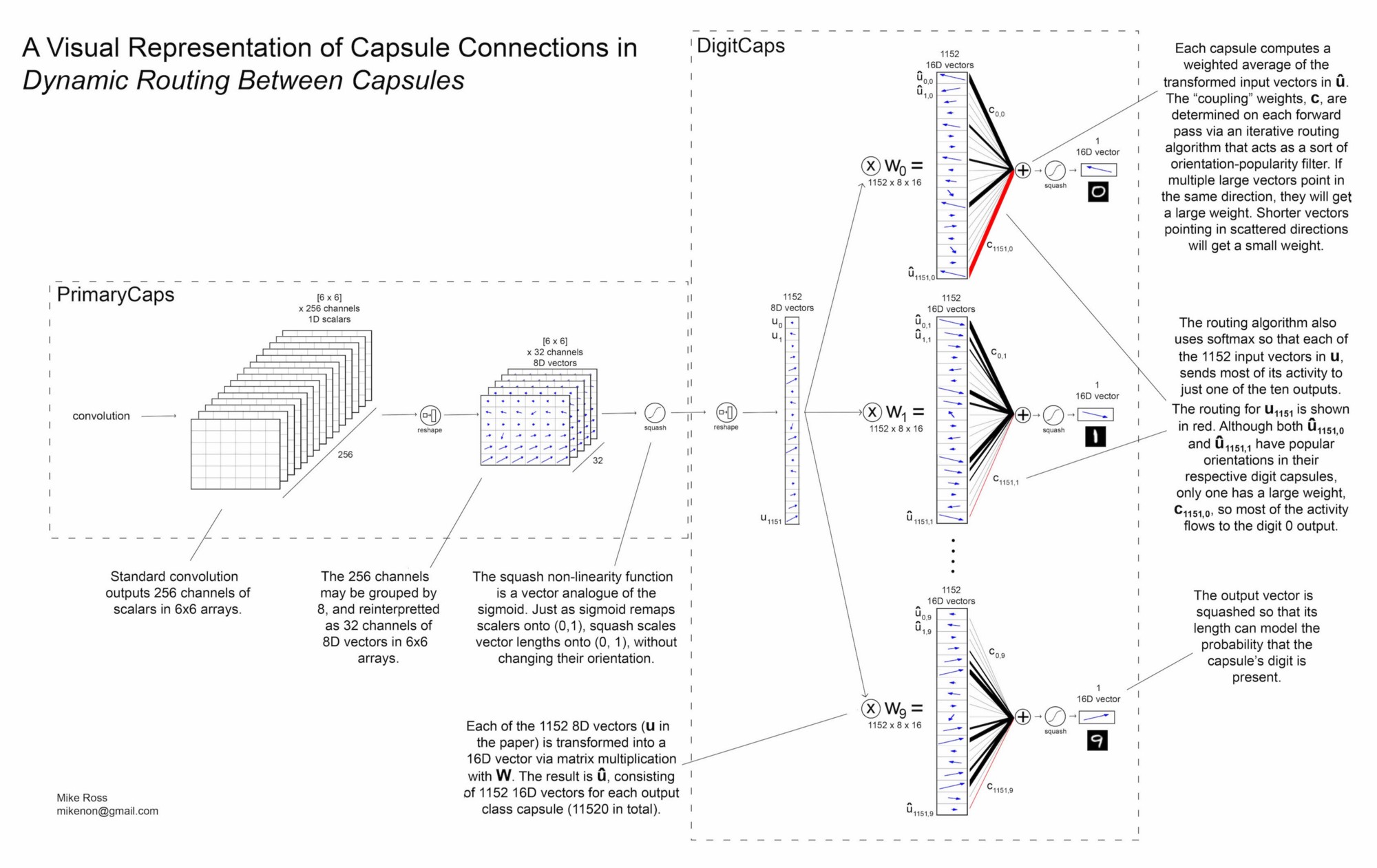
Caution, this figure has an error: instead of
Routing-by-agreement algorithm
For each the -D capsules are sumed up in a way that highly significant capsules with good predictions are weighted profoundly, and less significant capsules have less influence on the next capsule layer (Hinton et al., 2017). Hinton’s paper (Hinton et al., 2017) introduces a routing by agreement algorithm, that iteratively sets these weights, , and serves as a better way than max pooling to prioritize the dominant features, while at the same time preserving the less relevant data.
For every capsule in layer we have the prediction available, which is calculated by (150).
On the one hand, if the entity represented of capsule in layer is not related in any way to the higher level entity of capsule in layer , then will only have marginal impact, thus it is the goal of (1) to assign only marginal .
On the other hand, if many capsules in layer have similar for capsule in layer , then the corresponding will be major, because the capsules agree on what the object or entity of an object looks like, thus there is no need to send large weight to any other capsule. This would only cause noise.
With their calculation the capsules in layer try to predict the capsule in layer .
3.2.5 Example
In the following we follow up an examplel, introduced by (Géron, 2017), to better understand the dynamic routing between capsule.
Suppose a boat image such as in (12) is the input to CapsNet. As we see in (13), a triangle capsule (blue) and a rectangle capsule (black) become active. The corresponding activity vectors are present, the orientation marks the instantiation of that entity and the length marks the probability. Note that other image areas will result in short vectors for these two specific capsules, we omit these in the framework for the sake of simplicity.


Suppose the capsule class layer consists of only two capsule classes: one capsule identifying houses, the other identifying boats.
For :
According to the orientation of , the house capsule in layer , will predict an upside-down house, this is stored in . The information explaining the way the roof fits to the house is stored in the weight matrix .
On the other hand, the boat capsule predicts a slightly tilted boat for , this is stored in . The information explaining the way the sail fits to the boat is stored in .
For :
According to the orientation of , the house capsule will recognize a slightly tilted house, this is stored in . Whereas the boat capsule recognizes a slightly tilted boat from , this is stored in .
It is evident that the capsules in layer strongly agree on what a boat should look like ( and match) and strongly disagree on what a house should look like ( and differ). Therefore it is quite likely that the unfamiliar object is essentially a boat. Both capsules in layer should therefore send most of their output to the boat capsule in layer and only little to the house capsule .
Concretely, by applying the (1) routing-by-agreement algorithm, we can calculate appropriate weights in order to distribute high weights to well predicting capsules and low weights to poor predicting capsules.
We can think of and to be the activity vectors shown in figure (13).
Calculate each :
which is the input to algorithm (1). We can think of the to be the activity vectors shown in figure (13). Following the first step, we receive
(Hinton et al., 2017) has shown that the number of iterations can be to be working adequately. In the first iteration , applying softmax (69)(Wikipedia, 2018e) gives us
Softmax is similiar to the sigmoid function: delegate value between and and all values sum up to .
It must be (capsule in layer ) for all capsules in layer i.e. and .
The next step is calculating :
| (151) | ||||
| (152) |
Based on the vectors in figure (13), we can literally image how and look like:
must be a short vector pointing at o’clock, while must be a longer vector pointing at o’clock.
By squashing and , we receive and . While maintaining the orientation, is now even shorter and is longer.
The can now be updated according to how much each agrees with . We use the dot product to measure this agreement (marked by ""), because the dot product of two vectors depends on their length and in what angle they relate to each other (Wikipedia, 2018b).
Now and have much greater value.
In iteration and , the weights and will be rated even higher, since they will have greater impact on (151),(152).
Finally, the next-layer capsules, of layer ,are returned: a short red capsule and long yellow capsule (13). These capsules represent the best over-all predictions made by all the primary capsules in layer .
For each class capsule , there are weight matrices. In addition, the routing-by-agreement algorithm needs to variables for and another variables for . For class capsules, this sums up to trainable parameters in the Digit Caps layer - the weight matrices are learned by backpropagation, the routing parameters are learned by routing-by-agreement.
Following up on (3.2.4), the D capsules are sumed up in the manner of such that each of the weights is properly set according to the agreement . Routing by agreement delivers not only suitable weights , but also returns - the result are D squashed class capsules , for each class digit.
3.2.6 Margin Loss
To allow the prediction of multiple classes, we use a separate margin loss, for each digit capsule :
| (153) |
with if and only if digit of class is present and , and .
If digit is on the input image and corresponding digit capsule ends up having longer length than , then we have no margin loss. If digit is not on the input image and corresponding digit capsule ends up being shorter than , then we have no margin loss. With we can regularize the loss for falsely classified digits.
3.2.7 Reconstruction as a regularization method
As (Hinton et al., 2017) proposes, we can add a reconstruction loss to encourage the digit capsules to construct the instantiation parameters of the input image. During training, all but the true activity vector are blocked out and this activity vector is then used to reconstruct the input image. This reconstruction system is called decoder (Hinton et al., 2017) and consist of fully-connected layers attached to DigiCaps, see figure (14). The true activity vector is fed into the decoder and the final layer consists of units representing the pixel values of the reconstructed image. We can add the minimization of the squared difference between the input image pixel values and the reconstructed image pixel values to the sum of margin losses, and receive a total loss function. The reconstruction loss is down-scaled by (Hinton et al., 2017), so that the margin loss is the dominating factor. We use backpropagation and a gradient descent optimizer (adam) to minimize the sum of the margin losses plus the squared error of the decoder (Hinton et al., 2017).


3.3 CapsNet Training
An image is fed into the Input Layer. Applying a convolutional layer leads to various conv filters that represent certain low level shapes and angles in the image. These filters are stacked to capsule layers and squashed, in which each capsule represents a low level entity of the image. The activity vectors of each capsule store the instantiation parameters of the entity, the length shows the probability of it existing. The capsules associated to the digit in the image have a striking longer length than the others. In what manner each of entity is part of a whole class i.e. in what spatial relationship each entity is connected to the whole object, is defined by the weight matrix . Each capsule is then multiplied with a weight matrix . The result is , again in which the well predicting capsules have long length. Then routing by agreement sets the weights according to how much agrees with the mean i.e. the well predicting capsules receive a higher weight and contribute greater than others. The algorithm returns a Digit Caps layer, namely D squashed capsules . These high level capsules store high level features of more complex form, concretely, the entire digit. The result of an input image is that the corresponding capsule has long length and the other capsules have short length. The length characterizes the probability of a digit in the image and yields a prediction.
As (Hinton et al., 2017) pointed out, one can analyze individual dimensions of a capsule to learn of what instantiation it is represented by. There are programs, such as (Hsu, November, 2017), that perturb the dimensions of a capsule, making visible which instantiation is associated with the stroke thickness, skew, width etc. This might help improve transparency and accountability, since each capsules instantiation in every capsule layer can be exposed (Shahroudnejad et al., February, 2018).
A tensorflow implementation of CapsNet for MNIST can be found at
https://github.com/MJimitater/CapsNet/blob/master/CapsNet.ipynb.
3.4 Performance and Evaluation
The number of trainable parameters (including bias units) in CapsNet presented for the MNIST dataset in (Hinton et al., 2017), figure (9), are:
- •
Convolutional layer:
- •
PrimaryCaps layer:
- •
DigitCaps layer:
- –
sum (without decoder):
- –
- •
Decoder: fully-connected layer:
- •
Decoder: fully-connected layer:
- –
sum (with decoder):
- –
Other than a slight pixel shift, no data augmentation is performed in Hinton’s paper (Hinton et al., 2017). The baseline to compare is a three convolutional layer CNN with kernels of size and stride of . The last layer is followed by two fully-connected layers of size , and finally the output class layer of units, softmax activation, dropout, and adam optimizer (Hinton et al., 2017). The baseline sports million trainable parameters, however the paper (Hinton et al., 2017) is not entirely clear on how this number is calculated. The major property is to design the baseline to have best possible performance on MNIST wile keeping computation cost on a similar level to CapsNet.

The CapsNet’s architecture is the same as the one disussed in (9). As figure (16) of (Hinton et al., 2017) shows, CapsNet scores lower error rates than the baseline. The presented results also show the importance of the reconstruction decoder. It enforces the object’s instantation to be "encapsulated". The number of routing iterations also has an effect: a major positive effect with decoder, a minor negative effect without decoder.
Eventhough (Hinton et al., 2017) mentions notable performance of CapsNet on the MultiMNIST dataset and on the CIFAR10 dataset, concretely that the error rates match the ones of when standard CNNs first were applied to these datasets. CapsNet is a new artificial neural network architecture and is subject to further improvements to come.
(Mukhometzianov & Carrillo, May, 2018) gives insights to more extensive performance testing of CapsNet. The CapsNet as in figure (9), excluding the decoder subnetworks, was applied to several large datasets, such as Yale Face Database B (University, 2018) with classes, BelgiumTS traffic signs dataset (Timofte et al., 2011) with classes and CIFAR- (Krizhevsky, 2009) with classes, among others.
As baseline, different CNNs were used, including modified LeNet (LeCun et al., 1998) and Resnet (He et al., December, 2015).
On these large datasets with many more classes than MNIST, the baseline CNNs outperform CapsNet in both accuracy and average training time using GPU computing power (Mukhometzianov & Carrillo, May, 2018).

Regarding computational cost, CapsNet requires a lot more than CNNs. This is due to the fact that capsules output higher dimensional activity vectors with instantiation parameters than just scalar products, causing greater GPU memory usage.
There are three drawbacks presented by (Mukhometzianov & Carrillo, May, 2018):
First of all: for complex images, even higher dimensional capsules are needed to store all instantiation parameters, -D or even -D capsules. This would need further powerful GPUs with more memory to fit the capsule sizes.
Second of all: CapsNets achieve good accuracy with small datasets of simple complexity, but fail to hold up with CNNs at large complex datasets. It turns out that on complex datasets CapsNet also need many training images, this equalizes the hope for needing less training images. This hope only holds for simple and less complex images, as researched by (Mobiny & Nguyen, June, 2018). CNNs do possess undesirable properties e.g. lack of equivariance, however, on complex datasets, training with transformed images can solve this (Wikipedia, 2018c).
Third of all: increasing the size of the input images drastically increases computational cost. Downsizing is only a limited option, since it implies loss of information.
As investigated by (Afshar et al., March, 2018), modified CapsNets perform decently better than baseline CNNs in MRI brain tumor classification, as capsules handle small datasets well, despite the complexity in the images. Equivariance helps CapsNet to classify brain tumors more accurately than CNNs.
We can adhere that the success of CapsNets depend on the specific image application. It is yet to be researched in how far the image complexity matters, as well as the number of classes, the number of capsule layers and other hyperparameters.
As (Mukhometzianov & Carrillo, May, 2018) points out, it becomes clear that CapsNets are at an early stage of development and lack scalability, as CNNs were too when they first were applied (Wikipedia, 2018c). Further improvements are needed to boost accuracy and ameliorate computational cost, like done by (Mobiny & Nguyen, June, 2018). Several modifications have already been introduced by Hinton in an updated paper (Hinton et al., May, 2018) e.g. matrix capsules which group capsules to form part-whole relationships, rather than having weight matrices for this. Further testing and modification of hyperparameters is needed for CapsNet to utilize its full potential.
References
- Afshar et al. (March, 2018) Afshar, Parnian, Mohammadi, Arash, and Plataniotis, Konstantinos N. Brain tumor type classification via capsule networks. March, 2018. URL https://arxiv.org/pdf/1802.10200.pdf.
- Avrutskiy (December, 2017) Avrutskiy, V.I. Backpropagation generalized for output derivatives. December, 2017. URL https://arxiv.org/pdf/1712.04185.pdf.
- Bourdakos (February, 2018) Bourdakos, Nick. Understanding capsule networks - ai’s alluring new architecture. February, 2018. URL https://medium.freecodecamp.org/understanding-capsule-networks-ais-\ alluring-new-architecture-bdb228173ddc.
- Brownlee (September, 2016) Brownlee, Jason. How to improve deep learning performance. September, 2016. URL https://machinelearningmastery.com/improve-deep-learning-performance/.
- Chevalyre (2017) Chevalyre, Yann. Cours data mining / machine learning by yann chevalyre, paris dauphine université. 2017.
- Dauphin et al. (June, 2014) Dauphin, Yann N., Pascanu, Razvan, Gulcehre, Caglar, Cho, Kyunghyun, Ganguli, Surya, and Bengio, Yoshua. Identifying and attacking the saddle point problem in high-dimensional non-convex optimization. June, 2014. URL https://arxiv.org/pdf/1406.2572.pdf.
- Fischetti & Jo (December, 2017) Fischetti, Matteo and Jo, Jason. Deep Neural Networks as 0-1 Mixed Integer Linear Programs: A Feasibility Study. December, 2017. URL https://arxiv.org/pdf/1712.06174.pdf.
- Goodfellow et al. (2016) Goodfellow, Ian, Bengio, Yoshua, and Courville, Aaron. Deep Learning. MIT Press, 2016. http://www.deeplearningbook.org.
- Géron (2017) Géron, Aurélien. Capsule networks (capsnets) – tutorial. 2017. URL https://www.youtube.com/watch?v=pPN8d0E3900&t=434s.
- He et al. (December, 2015) He, Kaiming, Zhang, Xiangyu, Ren, Shaoqing, and Sun, Jian. Deep residual learning for image recognition. December, 2015. URL https://arxiv.org/pdf/1512.03385.pdf.
- He et al. (February, 2015) He, Kaiming, Zhang, Xiangyu, Ren, Shaoqing, and Sun, Jian. Delving Deep into Rectifiers: Surpassing Human-Level Performance on ImageNet Classification. February, 2015. URL https://arxiv.org/pdf/1502.01852.pdf.
- Hinton et al. (May, 2018) Hinton, Geoffrey, Sabour, Sara, and Frosst, Nicholas. Matrix capsules with em routing. May, 2018. URL https://openreview.net/pdf?id=HJWLfGWRb.
- Hinton et al. (2017) Hinton, Geoffrey E., Sabour, Sara, and Frosst, Nicholas. Dynamic routing between capsules. 2017.
- Hsu (November, 2017) Hsu, Jeremy. A partial implementation of the capsule network from dynamic routing between capsules. November, 2017. URL https://github.com/JeremyCCHsu/CapsNet-tf.
- Hui (2017) Hui, Jonathan. Understanding dynamic routing between capsules (capsule networks). 2017.
- Janocha & Czarnecki (February, 2017) Janocha, Katarzyna and Czarnecki, Wojciech Marian. On loss functions for deep neural networks in classification. February, 2017. URL https://arxiv.org/pdf/1702.05659.pdf.
- Kaggle (2014) Kaggle. Cats vs. dogs. 2014. URL https://www.kaggle.com/c/dogs-vs-cats.
- Karpathy & Johnson (Spring, 2018) Karpathy, Andrej and Johnson, Justin. Cs231n convolutional neural networks for visual recognition. Spring, 2018. URL http://cs231n.github.io/convolutional-networks/.
- Krizhevsky (2009) Krizhevsky, Alex. Learning multiple layers of features from tiny images. 2009. URL https://www.cs.toronto.edu/~kriz/cifar.html.
- Lecun et al. (1989) Lecun, Yann, Boser, B., Denker, J.S., Henderson, D., Howard, R.E., Hubbard, W., and Jackel, L.D. Handwritten Digit Recognition with a Back-Propagation Network. 1989. URL http://yann.lecun.com/exdb/publis/pdf/lecun-90c.pdf.
- LeCun et al. (1998) LeCun, Yann, Bottou, Leon, Bengio, Yoshua, and Haffner, Patrick. Gradient-based learning applied to document recognition. 1998. URL http://yann.lecun.com/exdb/publis/pdf/lecun-01a.pdf.
- medium (2017) medium. relu operation. 2017. URL https://medium.com/data-science-group-iitr/building-a-convolutional-neural-network\-in-python-with-tensorflow-d251c3ca8117.
- Mobiny & Nguyen (June, 2018) Mobiny, Aryan and Nguyen, Hien Van. Fast capsnet for lung cancer screening. June, 2018. URL https://arxiv.org/pdf/1806.07416.pdf.
- Mukhometzianov & Carrillo (May, 2018) Mukhometzianov, Rinat and Carrillo, Juan. Capsnet comparative performance evaluation for image classification. May, 2018. URL https://arxiv.org/pdf/1805.11195.pdf.
- Pechyonkin (February, 2018) Pechyonkin, Max. Understanding hinton’s capsule networks. part iv: Capsnet architecture. February, 2018. URL https://medium.com/@pechyonkin/part-iv-capsnet-architecture-6a64422f7dce.
- Peng et al. (2016) Peng, Min, Wang, Chongyang, Chen, Tong, and Liu, Guangyuan. Nirfacenet: A convolutional neural network for near-infrared face identification. 2016. URL http://www.mdpi.com/2078-2489/7/4/61.
- Picasso (1923) Picasso, Pablo. Portrait de femme au col d‘hermine. 1923. URL https://www.wikiart.org/en/pablo-picasso/untitled-1937-8.
- quora (2016) quora. convolutional operation. 2016. URL https://www.quora.com/How-common-is-it-for-neural-networks\-to-be-represented-by-3rd-order\-tensors-or-greater.
- quora (2017) quora. max pooling. 2017. URL https://www.quora.com/What-is-max-pooling-in-\convolutional-neural-networks.
- Ross (November, 2017) Ross, Mike. A visual representation of capsule network computations. November, 2017. URL https://medium.com/@mike_ross/a-visual-representation-of-capsule\ -network-computations-83767d79e737.
- Ruder (June, 2017) Ruder, Sebastian. An overview of gradient descent optimization algorithms. June, 2017. URL https://arxiv.org/pdf/1609.04747.pdf.
- Shahroudnejad et al. (February, 2018) Shahroudnejad, Atefeh, Mohammadi, Arash, and Plataniotis, Konstantinos N. Improved explainability of capsule networks: Relevance path by agreement. February, 2018. URL https://arxiv.org/pdf/1802.10204.pdf.
- Timofte et al. (2011) Timofte, Radu, Zimmermann, Karel, and van Gool, Luc. Multi-view traffic sign detection, recognition, and 3D localisation. Journal of Machine Vision and Applications, Springer-Verlag, 2011. https://btsd.ethz.ch/shareddata/.
- University (2018) University, Yale. Yale face database b. 2018. URL http://cvc.cs.yale.edu/cvc/projects/yalefaces/yalefaces.html.
- Wikipedia (2018a) Wikipedia. Receptive field. 2018a. URL https://en.wikipedia.org/wiki/Receptive_field#Visual_system.
- Wikipedia (2018b) Wikipedia. Dot product. 2018b. URL https://en.wikipedia.org/wiki/Dot_product.
- Wikipedia (2018c) Wikipedia. Convolutional neural network. 2018c. URL https://en.wikipedia.org/wiki/Convolutional_neural_network.
- Wikipedia (2018d) Wikipedia. Mnist database. 2018d. URL https://en.wikipedia.org/wiki/MNIST_database#Performance.
- Wikipedia (2018e) Wikipedia. Softmax function. 2018e. URL https://en.wikipedia.org/wiki/Softmax_function.
- Zhang (2016) Zhang, Zhifei. Derivation of backpropagation in convolutional neural network (cnn). 2016. URL https://pdfs.semanticscholar.org/5d79/11c93ddcb34cac088d99bd0cae9124e5dcd1.pdf.