Hydrodynamic model of BEC with anisotropic short range interaction and the bright solitons in the repulsive BEC

Solitons are famous nonlinear phenomena existing in various mediums. Being discovered on the water surface, solitons are found in plasmas [1], [2], [3], in lasers [4], in ultracold bosonic atoms [5], [6], in ultracold fermions [7], [8], in different setups of the condensed matter physics like spin waves [9], [10], [11], and charge density waves [12], [13], [14], [15]. Weak solitons observed over astronomical distances recirculating in an optical fibre loop [16]. Solitons show different features like attraction, repulsion, breaking up, merging, orbiting one another and the annihilation of two solitons [17], [18], [19], [20], [21]. Recently, it is demonstrated that solitons can absorb the resonant waves [22].

At the analysis of the nonlinear waves, many physical models of different physical systems lead to the nonlinear Schrodinger equation (NLSE) (such as the Gross-Pitasevskii (GP) equation) or the Korteweg–-de Vries (KdV) equation with cubic nonlinearity, where the nonlinearity is mostly caused by the interparticle interaction. For instance, the attractive short-range interaction in Bose-Einstein condensate (BEC) of neutral particles leads to the bright soliton existence (the area of the concentration amplification) while the repulsive interaction leads to the dark soliton formation (the area of the concentration rarefication). It seems that the Fermi pressure is the cause of the dark solitons appearance in the ultracold fermions [8], where the Fermi pressure gives the effective repulsion, but the nonlinearity is fractional. However, more generale models contain complex forms of nonlinearities, such as the quintic nonlinearity or the nonlocal nonlinearities. Generalised models predict existence of the bright soliton in mediums with repulsive meanfield interaction [23], [24].

There are two kinds of the nonlocal nonlinearities: the integral nonlinear term, like the dipolar BEC model [25], [26], [27], and the nonintegral nonlinearities containing spatial derivatives of the macroscopic wave function [28], [29], [30].

A model with nonlocal nonlinearity containing spatial derivatives is suggested in this paper at the analysis of the anisotropic short range interaction in the atomic BEC. Particularly, the paper is focused on study of the bright solitons in the repulsive BEC and the anisotropy of their properties.

Recent experiments with the BEC of rare-earth elements demonstrated phenomena requiring new physics for their explanation. It seems that it requires consideration of the quantum fluctuations in BEC in addition to the standard (meanfield) short-range interaction (SRI) and dipole-dipole interaction. To some extend, the ”constructive” three-particle interaction [31], [32], [33], [34], [35], [36] described by the fifth-order nonlinearity in the Gross-Pitaevskii equation was applied to these phenomena [37]. However, the quantum fluctuations demonstrated better agreement with experimental data. All mentioned interaction and related to them quantum fluctuations are applicable to the alkali-earth (see Ref. [38] for ⁵²Cr) atoms and rare-earth atoms (see Ref. [39], [40] for dysprosium ¹⁶⁴Dy). However, the quantum Rosensweig instability is found for the rare-earth atoms. Hence, the following question can be formulated: is it quantitative or qualitative difference. The rare-earth atoms show a qualitative difference due to the anisotropy of the SRI. It shows that a model of the rare-earth atoms with the account of the anisotropic SRI is required. The analysis of the spectrum of Feshbach resonances in the rare-earth atoms demonstrates an extra feature: anisotropy of the quasi-potentials [41].

It is found that the quantum Rosensweig instability in BEC of lanthanides (which are atoms with relatively large dipole-dipole interaction) can be modeled by an effective NLSE with the local form of the quantum correlations [42], [43], [44]

where $\Psi$ is the macroscopic (effective) wave function,

is the potential of the magnetic dipole-dipole interaction [25], [26], [27], [45],

represents the coefficient at the fourth order nonlinear term caused by the quantum fluctuations [39], [42], [40], [46], where the quantum fluctuations are related to the SRI and the dipole-dipole interaction, and $\mu$ is the electric/magnetic dipole moment, $\theta$ is an angle in the spherical coordinates $r$, $\theta$, $\varphi$, $g=4\pi\hbar^{2}a_{s}/m$, $\epsilon_{dd}=a_{dd}/a_{s}$, $a_{dd}=m\mu_{0}\mu^{2}/12\pi\hbar^{2}$ is the dipole length [25], [40], $a_{s}$ is the scattering length of the short range interaction, $m$ is the mass of particle, $\hbar$ is the Planck constant, $\partial_{t}$ is the time derivative. The dipolar part of the quantum fluctuations is found in Refs. [47], [48].

For the complete analysis of the Rosensweig instability in the rare-earth atoms, the many-particle quantum hydrodynamics method is applied to the derivation of the model with anisotropic SRI.

This paper is organized as follows. In Sec. II the formulation of basic ideas of the many-particle quantum hydrodynamics method is presented. In Sec III the quantum stress tensor is calculated in the first order by the interaction radius. In Sec. IV the quantum stress tensor is calculated in the third order by the interaction radius. In Sec. V generalization of the Bogoliubov spectrum is demonstrated. In Sec. VI the hydrodynamic equations are rewritten for the plane-like nonlinear objects propagating at the arbitrary angle to the preferable direction crated by the anisotropic interaction. In Sec. VII is on a possibility of the reduction of the nonlocal nonlinearity to a local one. In Sec. VIII models the bright solitons in the repulsive BEC appearing due to the nonlocal nonlinearities. In Sec. IX a brief summary of obtained results is presented.

Derivation of the model is based on the many-particle Schrodinger equation containing the following Hamiltonian:

where $m_{i}$ is the mass of i-th particle, $\hat{\textbf{p}}_{i}=-\imath\hbar\nabla_{i}$ is the momentum of i-th particle, $U_{ij}=U(\textbf{r}_{i}-\textbf{r}_{j})$ is the potential of interparticle interaction, $V_{ext}(\textbf{r}_{i},t)$ is the potential of external field acting on particles.

Derivation of the model starts with the definition of the simplest collective variable which is the quantum concentration of particles. It appears as the quantum mechanical average of corresponding operator:

where $dR=\prod_{i=1}^{N}d\textbf{r}_{i}$ is the element of volume in $3N$ dimensional configurational space, with $N$ is the number of particles. Its evolution calculated with the application of the many-particle Schrodinger equation and Hamiltonian (4) leads to the continuity equation: $\partial_{t}n+\nabla\textbf{j}=0$. The last one gives the explicit form of the current:

Next, the evolution of current leads to the Euler equation [28]:

where the current is represented via the velocity field $\textbf{j}(\textbf{r},t)=n(\textbf{r},t)\textbf{v}(\textbf{r},t)$, $p^{\alpha\beta}$ is the thermal pressure caused by the local distribution of particles on states with non-zero energy: the thermal effects or the quantum fluctuations, $\sigma^{\alpha\beta}$ is the quantum stress tensor caused by the short range interaction (SRI), and $T^{\alpha\beta}=-(\hbar^{2}/4m)[\partial^{\alpha}\partial^{\beta}n-(\partial^{\alpha}n)(\partial^{\beta}n)/n]$ is the quantum Bohm potential (this is a simplified form suitable for the BEC, while the general form is presented by equation (17) in Ref. [28] and equation (10) in Ref. [49]). Tensor $\sigma^{\alpha\beta}$ appears at the calculation of the force field. It is assumed that the masses of all particles are equal to each other and written without subindex: $m$. Originally, in the Euler equation, the force field appears as follows

It can be symmetrized relatively pair of interacting particles

Next, introducing the coordinates of relative motion and center of mass for each pair of particles $\textbf{R}_{ij}=\frac{1}{2}(\textbf{r}_{i}+\textbf{r}_{j})$, $\textbf{r}_{ij}=\textbf{r}_{i}-\textbf{r}_{j}$, represent coordinates of $i$-th and $j$-th particles via $\textbf{r}_{ij}$ and $\textbf{R}_{ij}$ in equation (9).

The SRI is considered. Hence, the potential $U_{ij}$ and its derivatives $\partial_{\alpha}U_{ij}$ go to zero for the large interparticle distances $\textbf{r}_{ij}$. Therefore, equation (8) is nontrivial for the small values of $\textbf{r}_{ij}$. Consequently, we can expand equation (8) in the Taylor series on parameter $\textbf{r}_{ij}$. The $\delta$ functions and the $i$-th and $j$-th arguments of the wave functions are involved in the expansion. The zeroth term and the even terms are equal to zero due to the symmetry of the equation (8) relatively $i$-th and $j$-th particles. Hence, we deal with odd terms. In the simplest case, we restrict our analysis with the first and third terms on the interaction radius.

This paper is a development of the many-particle quantum hydrodynamic method which gives a representation of the many-particle quantum system described by the time-dependent Schrodinger equation in terms of the collective variables. This method suggested in [50] for the quantum plasmas is applied to derivation of the Gross-Pitaevskii equation and its nonlocal generalization in [28]. It is done with accordance with the earlier proved possibility of such kind of derivation [51]. In this context, it is interesting to mention work [52], where the quantum dynamics of finite ultracold bosonic ensembles based on the Born-Bogoliubov-Green-Kirkwood-Yvon hierarchy for equations of motion for few-particle reduced density matrices with the necessary truncation. The multiconfiguration time-dependent Hartree method for bosons equations of motion of [53] for the specific wave function ansatz as their starting point.

Considering the quantum stress tensor (QST) in the first order by the interaction radius find the following representation in terms of the many-particle wave function:

where $R^{\prime}=\{\textbf{r}_{1},...,\textbf{R}_{ij},...,\textbf{R}_{ij},...,\textbf{r}_{N}\}$ with $\textbf{R}_{ij}$ is located on the $i$-th and $j$-th places, but $dR^{\prime}=d\textbf{R}_{ij}d\textbf{r}_{ij}dR_{N-2}$, where $dR_{N-2}$ does not contain the contribution of the $i$-th and $j$-th particles.

The particles under consideration have a preferable direction resulting in the nonisotropic interaction. Being in an arbitrary state the system consist of particles with the arbitrary orientation. The summation in the quantum stress tensor on all pair of particles leads to the cancelation or at leats the decrease of the anisotropic part. However, if all particles oriented in the same direction the anisotropic part is not reduced. Moreover, the part of integral (10) and the QST in the higher orders containing $\textbf{r}_{ij}$ can be extracted as the common multiplier. This assumption allows us to go to the simplified representation of the QST presented by the next equation. Let us mention here that the considered particles posses the magnetic moment. Therefore, orientation of the particles relatively the SRI is related to the creation of the spin polarization in the system. In the simplest case, the preferable direction of the SRI coincides with the spin direction. If it has an angle with spin the spin polarization create a partial orientation. Hence the perpendicular parts would cancel each other, but the part of the anisotropic SRI parallel to the spin is not zero and contribute in the collective interaction. This part enters the model developed in this paper.

The quantum stress tensor can be represented in a form containing two-particle concentration

where $Trn_{2}(\textbf{r},\textbf{r}^{\prime})=n_{2}(\textbf{r},\textbf{r})$ is the trace of the function of two arguments, and

is the explicit form of two-particle concentration.

Considering even and axial symmetric anisotropic potentials, include the expansion of the potential on the spherical functions

find a generalization of the quantum stress tensor obtained in [28]

where $\textbf{e}_{\theta}$ is the unit vector in the spherical coordinate system $r$, $\theta$, $\varphi$. Presence of $r^{\alpha}r^{\beta}$ and $e_{\theta}^{\alpha}r^{\beta}$ under the integral shows that two terms from expansion (13) give a contribution. These are terms proportional $Y_{00}(\theta)$ and $Y_{20}(\theta)$. The second of them brings anisotropy in the model. However, the calculation of the tensor structure of the quantum stress tensor in the first order by the interaction radius shows cancelation of the term proportional to $Y_{20}(\theta)$. Hence, the anisotropy gives no contribution to the quantum stress tensor in the first order by the interaction radius even if anisotropic part of the potential is comparable with the isotropic one.

The two-particle concentration is calculated for the Bose-Einstein condensate in [28], where it is found that $Tr(n_{2}(\textbf{r},\textbf{r}^{\prime},t))=n^{2}(\textbf{r},t)$.

After all, obtain the standard result for the quantum stress tensor in the first order by the interaction radius:

where $g=\int U_{0}(r)d\textbf{r}$.

Substituting the found QST in the Euler equation, find the following result

where $p^{\alpha\beta}=0$ since bosons at the zero temperature are considered.

The Euler equation (16) appears together with the continuity equation presented above. Here, we represent the continuity equation via the velocity field:

Equations (16) and (17) correspond to the traditional Gross-Pitaevskii equation [54]:

with

where $\textbf{v}=\nabla\phi$.

The quantum hydrodynamic model of BEC of neutral atoms with the SRI considered up to the TOIR is developed in 2008 [28] for the isotropic potentials. Here it is considered for the anisotropic potentials.

An analog of equation (10) obtained in the TOIR is a large equation. Majority of the terms in this equation do not contribute in the BEC dynamics being related to the excited states (see Appendix A). For the BEC it simplifies to

Calculation of the tensor structure of the QST in the TOIR gives the following result

where $I_{0}^{\alpha\beta\gamma\delta}=\delta^{\alpha\beta}\delta^{\gamma\delta}+\delta^{\alpha\gamma}\delta^{\beta\delta}+\delta^{\alpha\delta}\delta^{\beta\gamma}$ is a symmetric tensor existing in the term describing isotropic part, and $I_{2}^{\alpha\beta\gamma\delta}$ is a nonsymmetric tensor, or more precisely, it is symmetric relatively permutations of the last three indexes, but it is not symmetric relatively permutations of the first index and other indexes. Tensor $I_{2}^{\alpha\beta\gamma\delta}$ has the following elements: $I_{2}^{xxxx}=I_{2}^{yyyy}=1$, $I_{2}^{zzzz}=-2$, $I_{2}^{xxzz}=I_{2}^{yyzz}=-2/3$, $I_{2}^{xxyy}=I_{2}^{yyxx}=I_{2}^{zzxx}=I_{2}^{zzyy}=1/3$ and allowed permutations of indexes, other elements are equal to zero. Equation (20) contains two interaction constants $g_{2,l}=\int r^{2}U_{l}(r)d\textbf{r}/24$, $g_{2,l}=\tilde{g}_{2,l}/24$, where $l=0$, $2$.

Present the Euler equation with the SRI considered up to the TOIR

Obviously, the found generalized Euler equation corresponds to an approximation generalizing the Gross-Pitaevskii equation.

Interaction constants $g$ and $g_{2,0}$ are defined by $U_{0}$. Hence, they contributions $g\partial_{\alpha}n^{2}/2$ and $g_{2,0}\partial_{\alpha}\triangle n^{2}/2$ can be compared. Let us introduce the radius of interaction $r_{0}$ in a way that the interparticle interaction $U_{ij}(\textbf{r})$ or at least $U_{0}(r)$ is negligible for $r>r_{0}$. Consider dimensionally reduced parameters $\hat{g}$ and $\hat{g}_{2,0}$ introduced as follows $g=r_{0}^{3}\hat{g}$ and $g_{2,0}=r_{0}^{5}\hat{g}_{2,0}$, so $[\hat{g}]=[\hat{g}_{2,0}]=erg$. We have $\hat{g}=\int U_{0}(r_{0}\xi)d^{3}\xi$ and $\hat{g}_{2,0}=\int\xi^{2}U_{0}(r_{0}\xi)d^{3}\xi$, where $\xi=r/r_{0}$ and $\xi<1$ for the area of the nontrivial values of the potential $U_{0}$. Therefore, the presence of $\xi^{2}$ under the integral in the definition of $\hat{g}_{2,0}$ decreases its value in compare with $\hat{g}$. It shows $\hat{g}_{2,0}\ll\hat{g}$. Our comparison shows that the first order by the interaction radius dominates over higher orders. However, interaction constant $g_{2,2}$ is defined by another part of the anisotropic potential $U_{2}$. Therefore, constants $g_{2,0}$ and $g_{2,2}$ can have different relationships $g_{2,0}>g_{2,2}$ or $g_{2,0}<g_{2,2}$. If function $U_{2}$ is large in compare with $U_{0}$ (the large dipole anisotropy limit) the parameter $\hat{g}_{2,2}=\int\xi^{2}U_{2}(r_{0}\xi)d^{3}\xi$ can be large in compare with $\hat{g}_{2,0}$ and comparable with $\hat{g}$.

Spectrum of the collective excitations propagating as the plane wave in the infinite uniform BEC generalizing the Bogoliubov spectrum is

The first term on the right-hand side is the short-range interaction calculated in the first order by the interaction radius existing in the original Bogoliubov spectrum. The second term is the quantum Bohm potential contribution. The third and fourth terms are caused by the TOIR. The third term is related to the isotropic part of the TOIR. The last term in this equation is caused by the anisotropic part of the short range interaction. The third and fourth terms give a generalization of the Bogoliubov spectrum caused by the short range interaction in the third order by the interaction radius.

Equation (23) is found from the hydrodynamic equations (17) and (22). Derivation of equation (23) is made in the linear approximation on the small perturbations of the hydrodynamic functions relatively to the equilibrium state $n_{0}$, and $\textbf{v}_{0}=0$. Hence, the hydrodynamic variables are expressed as follows: $n=n_{0}+\delta n$, and $\textbf{v}=0+\delta\textbf{v}$. The perturbations are presented in the following form: $\delta n=N\exp(-\imath\omega t+\imath k_{x}x+\imath k_{z}z)$, and $\delta\textbf{v}=V\exp(-\imath\omega t+\imath k_{x}x+\imath k_{z}z)$, where $N$ and $V$ are the amplitudes of the perturbations.

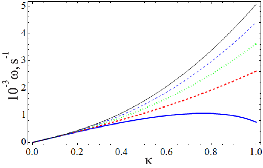
The terms proportional to $k^{4}$ dominate in the short-wavelength limit (the last three terms in equation (23)). The second term is positive. The third and fourth terms can be negative and they can overcome the second term. Hence, the short-wavelength instability can occur in the BEC due to the interaction in the third order by the interaction radius.

Presented comparison of three terms demonstrates that the parameter $\hbar^{2}/4mn_{0}$ is the natural unit for the interaction constants $g_{2,0}$ and $g_{2,2}$. Introduce corresponding dimensionless interaction constants $G_{2,0}=4mn_{0}g_{2,0}/\hbar^{2}$ and $G_{2,2}=4mn_{0}g_{2,2}/\hbar^{2}$.

Focus on the isotropic regime $g_{2,2}=0$. The repulsive SRI $g>0$ leads to the long-wavelength stability of the Bogoliubov spectrum. However, short-wavelength instability can exist if $G_{2,0}$ is larger then the quantum Bohm potential contribution $1$, where $G_{2,0}>0$ for the repulsive interaction since interaction constants $g$ and $G_{2,0}$ are the moments of the same partial potential $U_{0}$. If $1>G_{2,0}>0$ the spectrum (23)) is stable, but the frequency $\omega$ decreases in the area of large $k$ in compare with the first order by the interaction radius approximation.

Interaction constant $g_{2,2}$ is the moment of the second partial potential $U_{2}$. Therefore, it does not have direct relation to $g_{2,0}$. Hence, it is possible to have positive or negative $g_{2,2}$ at the positive $g_{2,0}$. Anyway, angle dependence of the last term in equation (23) gives different signs of the last term depending on the wave propagation direction.

Negative contribution of the TOIR in the square of frequency is demonstrated in Fig. 1. Changing direction of wave propagation we change the relative contribution of the TOIR. If angle is small enough and the TOIR interaction constants are large enough the frequency get the zero value at some wave vector $\kappa>1$. Spectrum becomes imaginary and condition for an instability occurs (see Fig. 2).

The instability can be caused by the isotropic part of the TOIR. However, in accordance with the described estimations, the anisotropic interaction constant can be larger then the isotropic TOIR constant. Therefore, the instability is easier detectable in the BEC of atoms with the anisotropic interaction.

Consider the wave propagation in the direction $h$ which has angle $\theta$ with the anisotropy axis (the $z$-axis). Change of coordinate in $h$ direction corresponds to the change of $x$ and $z$ (it is assumed that $y=0$) in accordance with the following relation $h=x\sin\theta+z\cos\theta$. The velocity field perturbations in the direction $h$ has corresponding form $v_{h}=v_{x}\sin\theta+v_{z}\cos\theta$.

The continuity equation transforms in the following way for the perturbations propagating in direction $h$

and

since $\partial_{x}f=f^{\prime}\sin\theta$, and $\partial_{z}f=f^{\prime}\cos\theta$, where $f=f(h)$ an arbitrary hydrodynamic function $n$, $v_{x}$, $v_{z}$ or their combination as a function of coordinate $h$, and $f^{\prime}=df/dh$.

Corresponding modification is found for the $x-$ and $z-$projections of the Euler equation

and

The $y-$ projection of the Euler equation is not involved.

Multiply equation (28) on $\sin\theta$ and equation (29) on $\cos\theta$ and combine obtained equations to get equation for $\partial_{t}v_{h}$:

Equation (30) shows that the third order on the interaction radius allows to introduce a single effective constant combining isotropic and nonisotropic parts

Hence, the last two terms in equation (30) can be written in the following way $\frac{g_{2}}{2}(n^{2})^{\prime\prime\prime}$.

Dimensionless form of parameter $g_{2}$ is presented in Fig. 3 and 4 for chosen values of $g_{2,0}$ and $g_{2,2}$. It is found that parameter $g_{2}$ can change the sign. Hence, the repulsion existing at small angles and positive $g_{2,i}$ can be changed by the attraction for the large enough $g_{2,2}$ (see Fig. 4).

Here we apply a method of nonperturbative analysis of the excitations in BEC. It allows to consider the large amplitude bright soliton in the one dimensional attractive BEC. This method is a nonperturbative on the amplitude of the excitations. However, below, we explicitly use the condition of the weak interaction in the TOIR approximation in compare with the interaction in the Gross-Pitaevskii approximation (or the FOIR approximation).

The section VII addresses the large amplitude solitons. However, the nonperturbative methods are relatively complex. Hence, we consider a method of the nonlinear analysis of the small amplitude perturbations. There are several methods, but we use the reductive perturbation method [57], [58]. It is applied for the analytical demonstration of the bright soliton existence in the repulsive 1D BEC.

The bright solitons in the attractive BEC described above is the well-known phenomenon while the repulsive BEC provides condition for the dark soliton. Although, it is found that mediums with repulsive interaction (including repulsive BEC [23]) can support the bright solitons [23], [24] under the influence of additional effects such as the quintic nonlinearity or the TOIR nonlocal nonlinearity. This phenomenon is studied here in terms of the developed model.

The reductive perturbation method introduces a dimensionless parameter $\varepsilon$. It is an indicator of small value of the corresponding terms (see below equations (47) and (48)). This parameter is also used for the scaling of space and time variables. In our case the stretched variables include the expansion parameter in follows combination:

where $u$ is the phase velocity of the wave, $\varepsilon$ is a small nondimension parameter.

An operational relations are arisen from (45)

The decomposition of the concentration and velocity field involves a small parameter $\varepsilon$ in the following form:

and

Presented in (47) equilibrium concentration $n_{0}$ is a constant. We put expansions (46)-(48) in equations (27) and (30). Consequently, the system of equation is divided into systems of equations in different orders on $\varepsilon$.

Equations emerging in the first order by $\varepsilon$ from the system of equations (27) and (30) have the following form

References

- [1] M. Q. Tran, Phys. Scr. 20, 317 (1979).
- [2] K. E. Lonngren, Plasma Phys. 25, 943 (1983).
- [3] E. A. Kuznetsov, A. M. Rubenchik, V. E. Zakharov, Phys. Rep. 142, 103 (1986).
- [4] B. Garbin, J. Javaloyes, S. Barland, and G. Tissoni, Chaos 27, 114308 (2017).
- [5] M. I. Shaukat, E. V. Castro, and H. Tercas, Phys. Rev. A 98, 022319 (2018).
- [6] G. E. Astrakharchik and B. A. Malomed, Phys. Rev. A 98, 013631 (2018).
- [7] A. Syrwid, D. Delande, and K. Sacha, Phys. Rev. A 98, 023616 (2018).
- [8] T. Yefsah, A. T. Sommer, Mark J. H. Ku, L. W. Cheuk, W. Ji, W. S. Bakr, M. W. Zwierlein, Nature 499, 426 (2013).
- [9] A. D. Boardman, S. A. Nikitov, and N. A. Waby, Phys. Rev. B 48, 13602 (1993).
- [10] A. V. Bagada, G. A. Melkov, A. A. Serga, and A. N. Slavin, Phys. Rev. Lett. 79, 2137 (1997).
- [11] Z. Wang, A. Hagerstrom, J. Q. Anderson, W. Tong, M. Wu, L. D. Carr, R. Eykholt, and B. A. Kalinikos, Phys. Rev. Lett. 107, 114102 (2011).
- [12] A. Rojo-Bravo, V. L. R. Jacques, and D. Le Bolloc’h, Phys. Rev. B 94, 201120(R) (2016).
- [13] T. Matsuura, J. Hara, K. Inagaki, M. Tsubota, T. Hosokawa and S. Tanda, EPL 109, 27005 (2015).
- [14] S. A. Brazovskiiand, S. I. Matveenko, Sov. Phys. JETP 72, 492 (1991) (Zh. Eksp. Teor. Fiz. 99, 887 (1991)).
- [15] Yu. I. Latyshev, P. Monceau, S. Brazovskii, A. P. Orlov, and T. Fournier, Phys. Rev. Lett. 95, 266402 (2005).
- [16] J. K. Jang, M. Erkintalo, S. G. Murdoch, S. Coen, Nature Photonics 7, 657 (2013).
- [17] J. P. Gordon, Opt. Lett. 8, 596 (1983).
- [18] F. Reynaud, A. Barthelemy, Eur. Phys. Lett. 12, 401 (1990).
- [19] V. Tikhonenko, J. Christou, B. Luther-Davies, Phys. Rev. Lett. 76, 2698 (1996).
- [20] M. Shih, M. Segev, G. Salamo, Phys. Rev. Lett. 78, 2551 (1997).
- [21] W. Krolikowski, B. Luther-Davies, C. Denz, T. Tschudi, Opt. Lett. 23, 97 (1998).
- [22] A. V. Yulin, Phys. Rev. A 98, 023833 (2018).
- [23] P. A. Andreev, L. S. Kuzmenkov, Mod. Phys. Lett. B 26, 1250152 (2012).
- [24] Z. Wang, M. Cherkasskii, B. A Kalinikos, L. D. Carr, and M. Wu, New J. Physics 16, 053048 (2014).
- [25] T. Lahaye, C. Menotti, L. Santos, M. Lewenstein, and T. Pfau, Rep. Prog. Phys. 72, 126401 (2009).
- [26] L. Santos, G. V. Shlyapnikov, P. Zoller and M. Lewenstein, Phys. Rev. Lett. 85, 179 (2000).
- [27] M. A. Baranov, Phys. Rep. 464, 7 (2008).
- [28] P. A. Andreev, L. S. Kuz’menkov, Phys. Rev. A 78, 053624 (2008).
- [29] N. N. Rosanov, A. G. Vladimirov, D. V. Skryabin, W. J. Firth, Phys. Lett. A. 293, 45 (2002).
- [30] E. Braaten, H.-W. Hammer, and Shawn Hermans, Phys. Rev. A. 63, 063609 (2001).
- [31] T. Kohler, Phys. Rev. Lett. 89, 210404 (2002).
- [32] E. Braaten, H.-W. Hammer, and T. Mehen, Phys. Rev. Lett. 88, 040401 (2002).
- [33] A. Bulgac, Phys. Rev. Lett. 89, 050402 (2002).
- [34] H. P. Buchler, A. Micheli, and P. Zoller, Nat. Phys. 3, 726 (2007).
- [35] D. S. Petrov, Phys. Rev. Lett. 112, 103201 (2014).
- [36] P. A. Andreev, Int. J. Mod. Phys. B 27, 1350017 (2013).
- [37] P. B. Blakie, Phys. Rev. A 93, 033644 (2016).
- [38] T. Lahaye, T. Koch, B. Frohlich, M. Fattori, J. Metz, A. Griesmaier, S. Giovanazzi, T. Pfau, Nature 448, 672 (2007).
- [39] I. Ferrier-Barbut, H. Kadau, M. Schmitt, M. Wenzel, and T. Pfau, Phys. Rev. Lett. 116, 215301 (2016).
- [40] H. Kadau, M. Schmitt, M. Wenzel, C. Wink, T. Maier, I. Ferrier-Barbut, T. Pfau, Nature 530, 194 (2016).
- [41] A. Petrov, E. Tiesinga, and S. Kotochigova, Phys. Rev. Lett. 109, 103002 (2012).
- [42] D. Baillie, R. M. Wilson, R. N. Bisset, and P. B. Blakie, Phys. Rev. A 94, 021602(R) (2016).
- [43] F. Wachtler and L. Santos, Phys. Rev. A 94, 043618 (2016).
- [44] R. N. Bisset, R. M. Wilson, D. Baillie, P. B. Blakie, Phys. Rev. A 94, 033619 (2016).
- [45] F. Wachtler and L. Santos, Phys. Rev. A 93, 061603R (2016).
- [46] S. K. Adhikari, Laser Phys. Lett. 14, 025501 (2017).
- [47] A. R. P. Lima and A Pelster, Phys. Rev. A 84, 041604 (2011).
- [48] A. R. P. Lima and A Pelster, Phys. Rev. A 86, 063609 (2012).
- [49] P. A. Andreev, L. S. Kuzmenkov and M. I. Trukhanova, Phys. Rev. B 84, 245401 (2011).
- [50] L. S. Kuz’menkov, S. G. Maksimov, Theoretical and Mathematical Physics 118, 227 (1999).
- [51] L. Erdős, B. Schlein, H.-T. Yau, Phys. Rev. Lett. 98, 040404 (2007).
- [52] S. Kronke, and P. Schmelcher, Phys. Rev. A 98, 013629 (2018).
- [53] O. E. Alon, A. I. Streltsov, and L. S. Cederbaum, Phys. Rev. A 77, 033613 (2008).
- [54] F. Dalfovo, S. Giorgini, L. P. Pitaevskii, and S. Stringari, Rev. Mod. Phys. 71, 463 (1999).
- [55] P. A. Andreev, M. I. Trukhanova, Russian Physics Journal 53, 1196 (2011).
- [56] R. Fedele and H. Schamel, Eur. Phys. J. B 27, 313 (2002).
- [57] H. Leblond, J. Phys. B: At. Mol. Opt. Phys. 41, 043001 (2008).
- [58] H. Washimi, T. Taniuti, Phys. Rev. Lett. 17, 996 (1966).
- [59] K. V. Zezyulin, P. A. Andreev, and L. S. Kuz’menkov, Eur. Phys. J. D 67, 140 (2013).