Geometry of the Phase Retrieval Problem
Abstract
One of the most powerful approaches to imaging at the nanometer length scale is coherent diffraction imaging using X-ray sources. For amorphous (non-crystalline) samples, raw data collected in the far-field can be interpreted as the modulus of the two-dimensional continuous Fourier transform of the unknown object. The goal is then to recover the phase through computational means by exploiting prior information about the sample (such as its support), after which the unknown object can be visualized at high resolution. While many algorithms have been proposed for this phase retrieval problem, careful analysis of its well-posedness has received relatively little attention. In this paper, we show that the problem is, in general, not well-posed and describe some of the underlying issues that are responsible for the ill-posedness. We then show how this analysis can be used to develop experimental protocols that lead to better conditioned inverse problems.
keywords
phase retrieval, ill-conditioning, well-posedness, transversality, non-negativity, HIO, difference maps.AMS
49N45, 94A08, 92C55, 94A12, 65R32, 65H991 Introduction
With the increased accessibility of high energy, coherent light sources, there has been a resurgence of interest in inverse imaging problems where the measurement can be interpreted as the modulus of the Fourier transform of an unknown object (see, for example, [14, 16, 17, 19, 28, 29, 31, 9]). In a typical set-up, an object with electron density is irradiated with a planar beam of coherent x-rays and a measurement of the scattered wave is made in the far field, i.e. the Fraunhofer regime. The wave’s phase information is not directly measurable, and the data collected are interpreted as samples of the intensity of the Fourier transform, . The reconstruction problem is then largely reduced to that of “recovering” the phases of the complex numbers . This experimental approach is referred to as coherent diffraction imaging (CDI).
Remark 1.1.
The phase retrieval problem came to prominence in x-ray crystallography, where is assumed to be a periodic function with some unit cell and are the coefficients of a discrete Fourier series, defined only on a regular lattice. In this context, without additional information, the phase retrieval problem is obviously ill-posed. One can assign any value to the phase of each to produce a periodic image. To circumvent this problem, for sufficiently small molecules, direct methods that rely on the non-negativity of the electron density and algebraic relations (Karle-Hauptman determinants) proved to be very powerful [30]. For larger structures, a variety of experimental approaches have been introduced to supply additional information that permits the reconstruction of the phase information needed to reconstruct the original crystal [24].
In the present paper, we are interested in the setting where is an essentially arbitrary, but compactly supported, function. The study of this problem dates back to 1952, when Sayre noted that for amorphous non-crystalline objects, one may obtain values of the intensity on a finer mesh than in the periodic case [34], since the spectrum is continuous. In essence, he proposed that one “over-sample” by a factor of two in each direction then recover as the solution to an overdetermined, constrained nonlinear least squares problem. The constraints come from some prior knowledge of , such as its support, whether it is non-negative, etc. It turns out that Sayre’s conjecture is essentially correct in more than one spatial dimension. More precisely, a finite approximation to phase retrieval problem introduced below in Section 1.1, with support as the auxiliary information, has a solution, generically unique up to “trivial associates;” see [3, 21, 22, 9]. In the continuum case, the trivial associates are obtained by applying operations to that leave invariant: translations ( for some ) and inversion ().
The most common additional information used in phase retrieval is a support constraint: that is nonzero only within some closed and bounded region in . It is with reference to an estimate for the support of that one speaks about over-sampling its magnitude Fourier transform. If is the smallest rectangle covering , then the Fourier data must be sampled on a grid fine enough to represent a periodic function with fundamental cell a rectangle whose side lengths are twice those of . In the phase retrieval literature, this is called “double oversampling.” In fact some degree of oversampling is clearly needed so that the sampled data contains adequate information about the support of for reconstruction to be possible. Double oversampling is the assumption required for the proof of the basic uniqueness theorem (Hayes’s theorem) in coherent diffraction imaging; it also allows the autocorrelation function of
| (1) |
to be reconstructed from the magnitude Fourier data without aliasing artifacts.
The earliest practical method for solving the phase retrieval problem is a variant of the alternating projection algorithm due to Saxton and Gerchberg [20]. The basic idea, which was first introduced in the context of Banach spaces by von Neumann as a method to find the intersections of convex sets, is quite general. In phase retrieval we let denote the collection of images with the given magnitude Fourier data and let denote the set of images which satisfy the support constraint. Given a function , projection onto corresponds to computing its Fourier transform , keeping the phase information from and replacing the modulus with the measured data . We denote this operator by . Projection onto corresponds to multiplying by the characteristic function of . We denote this operator by . Alternating projection can then be written as the following iteration:
| (2) |
with some initial guess .
This algorithm has a long history when and are convex sets, which we do not seek to review here (see, for example, [7]). It has also received a lot of study in the non-convex setting [2, 8, 10]. Unfortunately, alternating projection often converges to fixed points unconnected to the reconstruction problem at hand. To overcome this, Fienup proposed a new class of so-called hybrid input-output (HIO) algorithms [8, 18, 19], which were placed into the larger framework of difference-maps by Elser and collaborators, see [16, 17]. The fixed points of these algorithms all specify correctly reconstructed objects. We will describe this method in detail below in sections 4 and 5. Note that methods from continuous optimization have also been applied to this problem; see [31].
Despite the enormous effort that has gone into finding robust algorithms, the state of the art is generally unsatisfactory and reconstructions are typically not very accurate. That is to say, the phase retrieval problem with a support constraint has all the hallmarks of an ill-posed problem. Our main purpose in this paper is to describe recent work aimed at understanding what aspects of the phase retrieval problem render it ill-posed, and how this knowledge can be used to modify the experimental protocols to obtain better conditioned inverse problems.
Remark 1.2.
The phase retrieval problem sometimes refers to the more general setting where is unknown and measurements are of the form
for some set of querying functions . Here, denotes the inner product of the two functions. If the phase information were available, then solving for would correspond to a linear least squares problem. Without the phase information, the problem is non-convex. When the map from to is invertible, a variety of optimization methods have been developed based, for example, on semidefinite relaxation or gradient descent [12, 13]. Unfortunately, the phase retrieval problem of interest in x-ray scattering does not satisfy the necessary hypotheses for these methods to apply, namely that the forward map is injective and the solution is unique. The recent paper [1] contains a detailed analysis of phase retrieval in the invertible case and an interesting discussion of stability in that context.
1.1 The Discrete Classical Phase Retrieval Problem
For the sake of simplicity, we analyze a finite-dimensional analogue of the phase retrieval problem described above, which, in the limit of infinitely many samples, converges to the continuum problem. We assume that is real valued, and imagine that the unknowns are the samples where are points in a finite cubical integer lattice, . Here is the ambient dimension ( in our examples, but 3D phase retrieval is also possible [14]). The vector denotes an image, which can be viewed as a uniform pixelization of a density function lying in . We use the notation to denote the set of all possible such images. Using as the index set is somewhat non-standard in the engineering literature.
The measured data values are modeled as , where
| (3) |
is the usual -dimensional discrete Fourier transform (DFT) taking the pixel values to frequency data. We call magnitude DFT data, and denote the data vector by . We define the measurement map, by setting
| (4) |
Remark 1.3.
One may connect the above discrete model to the continuous case as follows. From (3), the indices are -periodic in each dimension. Let be the periodic folding of into the origin-centered cube . Then define the spatial frequencies for , which lie in the cube . The sum in (3) can be interpreted as approximate samples of , where the Fourier integral over has been approximated by a -point trapezoid quadrature (in each dimension) at the nodes . Thus for a continuous function the sequence tends to the exact Fourier transform as . An alternative (but less physically realistic) interpretation is: (3) gives point samples of the exact Fourier transform of a “sum of point masses” scatterer model .
The advantage of a discrete model over the continuous one is that it admits, given a support condition to be presented shortly, an exact solution that is generically unique up to trivial associates. In contrast, for the continuous problem, given any finite collection of samples of , there is an infinite dimensional space of functions with these Fourier coefficients, which also satisfy the support constraint.
Definition 1.
Given a magnitude DFT data vector , the magnitude torus, denoted by , is the collection of images in with this magnitude DFT data, i.e.
| (5) |
Remark 1.4.
Note that is either empty (if does not obey the inversion symmetry demanded by (3) for a real image), or is a real torus, or union of tori, of dimension equal to approximately half of the cardinality of . The reason for the approximate nature, and the possible existence of multiple connected components (which are all tori), is the fact that some data is forced to obey various symmetries; for example is always real, whereas most DFT data is generically complex. Vanishing DFT coefficients also lower the dimension of the torus.
The prior information about the image is encoded as a second set . The discrete classical phase retrieval problem is then the problem of finding points in the intersection ; see Fig. 1. For an image we denote its true support by
| (6) |
If then we say that is an estimate for the support of , and let
| (7) |
This is clearly a linear subspace of .
To define the operations in the finite, discrete case that generate the set of trivial associates of an image we need to extend the image to be -periodic. That is, the integer indices are defined mod in each dimension. With this understood, the image is defined for all with its restriction to representing a single period. We call such images -periodic. This is consistent with the formula for the DFT, which defines for all and the inverse formula, which defines for all as -periodic images.
With this periodic extension, the operations that generate the trivial associates are:
- 1.
If , then the translate of by is defined by its components
(8) - 2.
The inversion is defined by its components
(9)
Each image in the set of all trivial associates has the same magnitude DFT data as .
We now state a well-known uniqueness theorem due to Hayes [3, 21, 22], concerning the support constraint. If is contained in a rectangular subset of , with side lengths at most half the corresponding side-lengths of , i.e. at most , and , then the set is finite, and generically consists of trivial associates of a single point in this set.
Definition 2.
An image with support , for a set as above, is said to have small support.
Note that small support corresponds to the density function having support lying within a -dimensional cube of side length 1.
In some experimental situations one has a constraint , where
| (10) |
This auxiliary condition alone does not uniquely specify a set of trivial associates, or even a finite set. It is easy to show, however, that the squared magnitude data are the DFT coefficients of the autocorrelation image
| (11) |
In [6] we prove that if the support of is sufficiently small, then the set of non-negative images in is finite, and generically consists of trivial associates of a single element. This follows because, for , if the support of is sufficiently small, as a subset of then it provides a non-trivial upper bound on the support of , for which we can conclude uniqueness, up to trivial associates. As all points have the same autocorrelation image, without a non-negativity constraint, the support of the autocorrelation image does not, in general, provide a bound on the support of the image itself. We refer to the problem of finding the intersection as phase retrieval with non-negativity constraints.
Definition 3.
We say that the set defined by some auxiliary conditions, is adequate if the intersection is a finite set for any in the range of . (Thus, if the support of is sufficiently small, then non-negativity of the image is adequate data for phase retrieval.)
1.2 Well-posedness of the Discrete Phase Retrieval Problem
The concept of well-posedness for an inverse problem comprises two distinct questions: the first is the uniqueness of the solution and the second concerns the continuity properties of the local inverse map near a solution. For the phase retrieval problem, uniqueness should be understood as uniqueness up to trivial associates.
Neither aspect of well-posedness has been analyzed in detail for the phase retrieval problem. From the proof of Hayes’ uniqueness theorem, it follows that there are pairs of images, , which are not trivial associates, with identical magnitude DFT data and support for which . Yet, since uniqueness is generic, we can find images, , as near to as we like for which the phase retrieval problem does have a unique solution. Moreover we can assume that the supports of are the same as those of . From this observation it is clear that, at any finite precision, this problem does not always have a unique solution, even up to trivial associates. A similar observation was made by Fienup and Seldin in [35].
A primary concern here is that of understanding what makes it difficult to find points in even if it is assumed that the set is selected so that this intersection consists of finitely many points. In coherent diffraction imaging, the cardinality of the index set is in the hundreds of thousands, millions, or even billions (depending on whether a two-dimensional or three-dimensional object is being imaged and at what resolution). High dimensionality certainly complicates the problem at hand, but it is not the root cause of its difficulty. Rather, it is the geometry near to points in that renders this problem so difficult. This sort of local geometry is usually discussed in terms of the relationship of the fibers of the tangent bundles to and at points of intersection. For the remainder of this discussion we focus on the support condition case , which is itself a linear subspace.
Definition 4.
For a point the fiber of the tangent bundle to at , denoted by , is the affine subspace of through that is the best linear approximation to near to .
Remark 1.5.
An embedded submanifold of a Euclidean space has a “best” approximating affine subspace if it is at least A magnitude torus is a product of round circles and is therefore a real analytic subspace of
Definition 5.
Let . The intersection of with is transversal at if
| (12) |
that is, the affine space intersects the linear subspace only at .
If the intersection is transversal, then the geometry of near to is accurately modeled by a neighborhood of in In this case, the conditioning of the problem of finding a point is determined by the angles between and If there are positive dimensional subspaces of and that make a very small angle with one another, then the condition number, though finite, will be very large.
For high dimensional non-linear submanifolds of one does not generally expect to have an explicit description of the fibers of the tangent bundle. It is a remarkable feature of magnitude tori that such a description is accessible. Using this description we can show that the intersections between and are typically not transversal. If the intersection at is not transversal, then is a positive dimensional affine subspace. In this case the local geometry of near to does not resemble that of the linearized problem does not have a unique solution. Formally speaking, the condition number of the non-linear problem is infinite. Moreover, in this case, linear analysis fails to adequately describe the behavior of algorithms for finding intersection points.
Above we defined as the “forward operator” (in the language of inverse problems), i.e. the measurement map from an image to its corresponding DFT magnitude data . The inverse image of a point is simply its magnitude torus . Suppose now that has small support contained in the set . Then, by Hayes’ theorem, the set is finite, and non-empty. This remains true if is replaced by a nearby point . Therefore, the map has a local inverse, defined on the manifold of consistent data , near to . We denote this local inverse by As noted above, the other issue that arises in a discussion of well-posedness is the continuity of this local inverse. In [6] we prove the following theorem.
Theorem 6.
The local inverse satisfies a Lipschitz estimate if and only if the intersection of with at is transversal.
By itself, the failure to have a local Lipschitz inverse leads to a kind of ill-conditioning. When the intersection is non-transversal, the local inverse is, at best, Hölder continuous of order , which implies an infinite condition number. In fact the number of accurate digits possible in the reconstructed image cannot exceed when the data is available with a relative precision of digits. For phase retrieval, it is often the case that (see Fig. 1(b) for an illustration with ). More critical, however, is that non-transversality stalls the convergence for standard reconstruction algorithms, even in the ideal case of noise-free data, as discussed in section 4.

1.3 Contents of the Paper
An outline of the paper follows: in sections 2 and 3, we discuss the geometry of phase retrieval with support constraints. We turn to the practical consequences of our analysis in sections 4 and 5, and extend the analysis to the case of non-negativity constraints in section 5.2. In section 6, we consider the possibility of alternate experimental protocols that yield better conditioned inverse problems. We draw heavily here on results from the text [6], which contains, among other things, complete proofs of the main theorems used (as well as more detailed numerical experiments).
2 The Tangent Bundle to
In this section we let denote an image with small support. The question of transversality of the intersection at concerns the relationship between the fiber of the tangent bundle to at and a linear approximation to the set . For any we let denote the fiber of the tangent bundle to at . The fiber of normal bundle at is the affine subspace through orthogonal to We have defined these fibers as affine subspaces of the ambient space and let denote the linear subspaces of so that
| (13) |
Recall that for where is an estimate for the support of , is a linear subspace and the intersection is transversal if and only if .
Remark 2.1.
If (see (10)) then the intersection lies on which is not a smooth submanifold of but rather a stratified space. This renders the concept of transversality more subtle to define. As the is “piecewise linear” in that it is locally a union of orthants in linear spaces of various dimensions, it again makes sense to say that the intersection is transversal provided that Since it is conceptually much simpler (and more general in its applicability), most of our discussion of transversality uses a support constraint as auxiliary information. In Section 5.2 we briefly discuss the transversality of the intersection with
2.1 The Tangent Bundle in the DFT Representation
The key to analyzing these intersections is to have an explicit, readily computable description of the fibers of the tangent bundle to In this section we give two such descriptions. The DFT (3), which we denote by , maps the torus onto a torus in defined by
| (14) |
Taking -derivatives gives a very simple description of the tangent bundle: for ,
| (15) |
where the standard basis vector has a in the th location and is otherwise zero. It is the “real-span” because is a real submanifold of
As the images, we consider are real, this is reflected in a symmetry of : for each index there is a conjugate index where for which
| (16) |
note that In fact, the fiber of the tangent bundle is the span of a smaller set of vectors:
| (17) |
The fiber of the normal bundle has a similar description:
| (18) |
Up to a scale factor, the DFT is a unitary map, and therefore though this is not a very explicit, or useful description.
2.2 The Tangent Bundle in the Image Representation
We now give a second description, in the image domain, of bases for the tangent and normal bundles to whose elements share many properties with that of the image itself. Recall that, for the translate, of by is defined in (8). Introduce the following images, which are the difference and sum of translates of the image by and
| (19) |
Theorem 7.
Suppose that is the DFT magnitude data of a real image, For any point , we have that
| (20) |
Remark 2.2.
The images are of course just trivial associates of , whose existence makes the solution of the phase retrieval problem non-unique. In fact the distances between the trivial associates are fairly large; an effective algorithm defined by a map with strong contraction properties would not have problems on this account. The theorem describes a far more insidious effect of the existence of trivial associates, as explained in the next paragraph: it often renders the intersections of and non-transversal. As we shall see in the next section, this adversely affects the continuity properties of the inverse map, which is entirely algorithm-independent. In Section 4 we see that it also vastly diminishes the contraction properties of the maps used to define phase retrieval algorithms, which inevitably leads to stagnation and even poorer reconstructions than would be expected from the results of Section 3.
Given an image, , there is a subset of so that is a basis for the vector space If is a realistic estimate for the support of , then there is usually a non-empty subset such that the tangent vectors also have support in . In this case
| (21) |
which implies that the intersection at is not transversal.
For a subset the -pixel neighborhood, of is defined to be
| (22) |
Once again this distance should be understood in the -periodic sense. A simple combinatorial argument shows that
| (23) |
showing that a looser support constraint leads to a greater failure of transversality.
2.3 The Convolution Property of
In this section we examine a surprising property of the tangent bundle to magnitude torus defined by a image that is a convolution of two other images, that is
| (24) |
In this section it is important to recall that we regard images in as periodic, i.e. as elements of with indices in representing a single period.
This discussion requires some additional notation. For we let
| (25) |
so that is the magnitude torus defined by and we let
| (26) |
Suppose that is chosen so that is a basis for If then we let
| (27) |
Recall that (periodic) discrete convolution is defined by
| (28) |
The support of a convolution satisfies
| (29) |
where we recall that if then The DFT coefficients of a convolution satisfy
| (30) |
It is an elementary computation to show that
| (31) |
For generic images, and a single index set can be used so that is a basis for and is a basis for Letting , it follows from (31) that
| (32) |
More succinctly we can write:
| (33) |
If we let
| (34) |
| (35) |
Suppose that is an image for which there exists an so that
| (36) |
The vector field then satisfies
| (37) |
On its face the condition in (36) seems very unlikely to hold for any as it is equivalent to the system of linear equations for :
| (38) |
Since and for an image with small support, the equations in (38) appear to be overdetermined.
It turns out that if is inversion symmetric, that is
| (39) |
then the basis vectors for satisfy the equations
| (40) |
For the case of an inversion symmetric image, half of the equations in (38) imply the other half, from which the following theorem follows easily.
Theorem 8.
Let be inversion symmetric, then the solution space to the equations in (38) has dimension at least
| (41) |
Remark 2.3.
This theorem also holds for images that are anti-symmetric, i.e. and images that are inversion symmetric (or anti-symmetric) with respect to any point in
An inversion symmetric image has real DFT coefficients, and therefore that phase retrieval problem for such an image reduces to the much easier sign retrieval problem. But suppose that is an arbitrary image with small support, and is inversion symmetric so that also has small support. The theorem along with (37) imply that
| (42) |
For non-negative images in any case, the sum is a reasonable estimate for The failure of transversality, with is inherited by from even though has no obvious symmetries.
2.4 Examples of the Failure of Transversality for Convolutions
The analysis in the previous section shows that for images that are convolutions with inversion symmetric images, the failure of transversality occurs even if we use the exact support of the image to define the support constraint. In order to diminish the effects of noise, it is a very common practice to multiply measured data by a smooth cut-off function, such as a Gaussian. Since our measurements are in the DFT domain, equation (30) shows that this is equivalent to convolving the unknown image with a Gaussian. Our analysis suggests that this makes the problem of recovering the phase much more difficult. In this section we present the results of numerical experiments that demonstrate this phenomenon.
For our numerical experiments, we use images defined by a sum of radial functions,
| (43) |
In the simplest case, each function is a scaled characteristic function of a disc,
| (44) |
where the intensities , radii , and centers are set randomly; see left side of Fig. 2(a). In this case the function is piecewise constant; in the imaging literature one would say that represents a hard object. The discrete image is then generated from point samples of on a regular grid. We also generate smoother images by (discrete) convolution of this with the discretely sampled Gaussian,
| (45) |
where controls the smoothness, and where is chosen to make . (The unsmoothed case we denote by .) In Figure 2 we show examples of such images with smoothness levels (unsmoothed), , and .

Since the smoothing in (45) results in full support, we instead set a threshold appropriate for finite-precision arithmetic, and define the support to be
| (46) |
The -pixel neighborhoods, of are defined as in (22). To see how depends on the degree of smoothing, , and the size of the support padding, , we generate 5 random samples, for each smoothness level Since the intersection dimension computation requires a dense SVD of a matrix of size , the study is limited to small images; we choose the image size so that the double oversampled image is . For these images and The dimension decreases when as the symmetries of forces certain DFT coefficients to vanish.
For each sample image, we numerically compute , an orthonormal basis for , and , an orthonormal basis for , and then compute the SVD of . In exact arithmetic, is the number of singular value, equal to 1. Since we work in finite-precision arithmetic, such singular values are only approximately 1. Figure 3 contains plots of Note that there is a sharp transition from singular values within of 1 to smaller ones, which is remarkably consistent across the samples. As the support of the Gaussian, (at machine precision) grows with this is essentially as predicted by Theorem 8.
We summarize these dimension measurements in Table 1. The dimensions shown correspond to the number of singular values greater than . The row is precisely as predicted in (23). The table also has a column where we have used the exact support, to define the support constraint. As predicted by Theorem 8, for the dimensions of these intersections are non-zero. As increases, the support of grows, and this produces a larger and larger intersection between and As increases the dimension of these intersections grow beyond the larger is, the more ways there are to obtain tangent vectors of the form so that In examples below we show that even a very low dimensional failure of transversality can lead to stagnation in standard reconstruction algorithms.
| smthns\supp | |||||
|---|---|---|---|---|---|
| 0 | 4 | 12 | 24 | 40 | |
| 18 | 34 | 54 | 78 | 106 | |
| 38 | 64 | 92 | 124 | 160 | |
| 61 | 88 | 120 | 156 | 196 | |
| 85 | 119 | 155 | 195 | 239 |
This experiment can be repeated using images defined as samples, of functions of the form
| (47) |
where
| (48) |
These functions increase in smoothness with but are not defined as convolutions. For each we produce 5 random choices of In this case we find that the dimensions of the intersections are independent of satisfying in this case for all In Figure 4 we show plots of for each choice with From these plots we see that does not depend on or the choice of example, and that the number of directions in which meets at very small angles does increase with These small angles also dramatically stall the convergence of standard algorithms for finding these intersections.
3 Transversality, Well-Posedness and Microlocal Non-uniqueness
We turn now to an analysis of the effects of a non-transversal intersection on the computational difficulty of the phase retrieval problem. While the results in this section are algorithm independent, they have direct implications about the loss of solution accuracy given finite precision data and computations. The results in this section are related to and, in part, inspired by those in [11] and [1].
3.1 Transversality and Well-Posedness
Recall from the introduction that denotes the measurement map . First note that this map is Lipschitz continuous in the -norm,
| (49) |
with , which follows from the Plancherel theorem for the DFT (3) and the triangle inequality. The inverse image of a point is the magnitude torus . Suppose that has small support contained in the set , then the set is finite, and non-empty, and the local inverse is defined on a neighborhood of in the set of consistent data .
As is typical in the field of inverse problems, in order for the problem to be locally well posed at it is necessary for this local inverse to be a Lipschitz map. That is, there must be a neighborhood of and a constant , such that for , we have the estimate
| (50) |
so that if and then
| (51) |
Now assume that is non-transversal at and let be a unit vector, then the definition of the tangent bundle, and (49), imply that there is a constant , dependent on , so that
| (52) |
In this case the best general bound one can hope for is that
| (53) |
This implies that the local inverse is, at best, Hölder continuous of order , and therefore has an unbounded condition number. As noted in the introduction, it also implies that if the measurements have significant digits, then, generally, it will be impossible to reconstruct an image with more than significant digits.
In [6], we prove the following result:
Theorem 9.
For an image , let denote the magnitude torus defined by . Suppose that for all . There are positive constants, , , so that, if and , then
| (54) |
if and only if .
The theorem says that, if a support condition is the auxiliary information that is available, and the DFT data is generic (non-vanishing), then the phase retrieval problem can only be well-conditioned near to if this intersection is transversal. This statement is intrinsic to the phase retrieval problem, i.e. is algorithm independent. The results in section 4 indicate that, with a realistic support condition, these intersections are very rarely transversal (see Table 1 and Figure 4 above). As our numerical experiments below show, this failure of transversality can also dramatically harm the convergence properties of standard algorithms.
3.2 -Non-Uniqueness
As discussed in the introduction, the solution to the phase retrieval problem with support condition is not always unique up to trivial associates. From the discussion in the previous section we already know that the conditioning of the phase retrieval problem depends subtly on the unknown image, and the precise nature of the auxiliary information. In this section we explore various ways in which this problem can fail to have a unique solution to a given precision Suppose that there are two images and a subset adequate for generic uniqueness, such that
- 1.
The norms but the minimum distance between trivial associates of and is much larger than
- 2.
The sets for
- 3.
then we say that the solution to the phase retrieval problem defined by the data is -non-unique. In the remainder of this section we describe two distinct mechanisms that lead to -non-uniqueness.
3.2.1 Consequences of Genuine Non-Uniqueness
The fact that a discrete image, with sufficiently small support, is generically determined by the magnitude DFT data is a consequence of the classical theorem that polynomials in two or more variables are generically irreducible over the complex numbers. If is the image, then its -transform is
| (55) |
where There is a minimal integer vector so that is a polynomial.
Suppose that is an image whose -transform, is reducible, in the sense that there are polynomials, in such that
| (56) |
for some integer vector If and are images with -transforms (up to a factor of for some ) then, up to a translation, where denotes discrete convolution. If no trivial associate of either or is inversion symmetric, then the image is not a trivial associate of and, typically, the minimum distance between the trivial associates of and is large. If and are non-negative, then so are and and the smallest rectangles containing each image coincide.
Suppose that and both have small support contained in a set which is small enough to generically imply uniqueness, up to trivial associates, and let be chosen with Because uniqueness is generic we can modify these two images to obtain generic images and so that the norms satisfy the estimates , , and , . The data defines both a phase retrieval problem with a unique solution, up to trivial associates, and an -non-unique problem. That is, we can construct images and with support in and nearly identical magnitude DFT data:
but satisfying


We conclude this section with an example of a pair of non-negative images, , with exactly the same support and magnitude-DFT data such that The minimum distance between trivial associates is about but the closest trivial associates have rather different supports. These images are obtained as described above with and non-negative images whose supports are inversion symmetric, but the images themselves are not. The left and middle images in Figure 5(a) show the central portion of and and the right image shows their common support. The left image in Figure 5(b) is the -magnitude-DFT of both images, the right image is the central portion of the difference of the two images.
What is striking about this example is how perfectly ordinary the images and their magnitude-DFT data look. The only criterion that we know of (in the continuum model) to exclude this phenomenon is that it cannot occur in an image with jump discontinuities, because the convolution of two bounded measurable functions is continuous. For the discrete model it is difficult to make this statement precise, as there are images where, say, is a “sum of -functions,” which provide counterexamples. Note that, for discrete images, a sum of -functions is modeled by an image with support in a set of isolated pixels. In fact such examples can be found in [35]. A complete (asymptotic) analysis of this problem might require an analysis, as tends to infinity, of the density of the subset of reducible polynomials of degree within the set of all polynomials of this degree. For results in this direction see [23]
3.2.2 Microlocal Non-Uniqueness
There is a second mechanism that leads to -non-uniqueness, which we call microlocal non-uniqueness. We now explain the mechanism underlying this phenomenon. For the construction, let be a set so that images supported in have small support. Let be an image that can be decomposed as a sum,
| (57) |
where the components have the following properties:
- 1.
For each we have
- 2.
Each pair has distinct spectral -support,
(58)
From the second condition, it follows that, for and a binary string, the set of images
| (59) |
all have the same DFT magnitude data to precision Indeed, we are also free to replace some of the with their inversions . For a realistic estimate of the support, images defined by a collection of small translations also have their supports within to precision . In this way a large collection of images, which are not trivial associates, can be constructed that belong to the intersection up to a fixed, very small, error. The data for any one of these images is -non-unique, for some fixed .
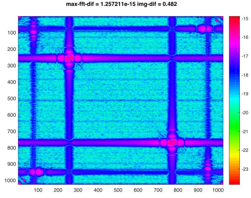
We close this section with an example of a pair images, whose difference is , but with identical support, and magnitude DFT data to precision In this example, which is shown in Figure 6,
Example 3.1.
In , let the four images through be defined by their components
| (60) |
where
| (61) |
and , so . Then we construct
| (62) | ||||
where the translation vectors are given by
Figure 6(a,b) shows a plot of and . The support sets are defined as In both cases this is a disk of diameter pixels, thus the support is small. Yet the magnitude DFT data of these images are equal to precision , thus phase retrieval is incapable of distinguishing from , even if the data is measured to, say, 12 digits of accuracy.


Remark 3.1.
The reader may note that our construction is somewhat pathological, since the DFT of the image consists of well-separated Gaussian “islands” of non-zero data, which leads to easier detection of this sort of -non-uniqueness. The examples in Section 3.2 are less pathological and this form of non-uniqueness is more difficult to detect. It remains an open problem to describe the class of images for which -uniqueness can be proven, even for very small values of
4 Algorithms for Phase Retrieval
We now see what the results of the previous sections imply about the behavior of standard algorithms used for phase retrieval. These algorithms are defined by iterating maps, which are, in turn, built from “closest point maps.” If is a subset of then is defined to be the point in closest to with respect to the Euclidean distance. If is a linear subspace then is the orthogonal projection. If is convex then is defined and continuous everywhere, whereas for a non-convex set, these maps are defined, and continuous, on the complement of a positive codimensional subset.
In the phase retrieval problem, let us assume that the unknown and its support are adequate in the sense of definition (3), with the magnitude torus defined by the DFT magnitude data . As a torus, is obviously not a convex set. The alternating projection method (2), which we write here in the form
| (63) |
is well known to be prone to converge to points that are not in The stable fixed points of the alternating projection map are points such that and jointly form a non-zero, local minimum of the Euclidean distance between the two sets. Empirically these exist in great profusion, and the alternating projection method rarely (if ever) converges to a point in See [6] for a more extensive discussion.
In an attempt to avoid such false local minima and improve convergence, a variety of modifications to the alternating projection map have been introduced that involve reflection operators as well as projections. Quite a few variants have appeared in the literature [8, 14, 16, 17, 19, 28, 29], and we will limit our attention to a special case of Fienup’s hybrid input-output (HIO) method [18], which is also a special case of the “difference map” approach due to Elser et al. [16]. Letting and now denote general sets, with closest point projections and , the map that we iterate is
| (64) |
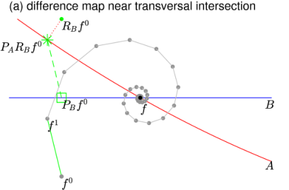
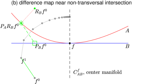
where is the “reflection” around defined by ; see Figure 7. This is Fienup’s HIO method with and a specific instance of Elser’s, difference map as well. If is a linear subspace, then is also the Douglas-Rachford map, which is defined to be
| (65) |
see [10].
Since we are not testing all possible HIO or difference map variants, we will call the specific method we use here a “hybrid iterative map.” If is a fixed point of then
| (66) |
in other words, the point lies in . The iterates are defined by , and approximate reconstructions are given by
| (67) |
If the iterates converge, then, assuming that is continuous at the limit point, the sequence converges to a point in
The fixed point set of can be much larger than the set of intersections. Given a point , we let
| (68) |
The center manifold defined by (see Figure 7) is then the set
| (69) |
The center manifold for any contains the part of the fixed point set for the map which “points to” Given an image with support in a small support set (see Definition 2), and choosing and , then the part of the center manifold near to is given by , and with . However the map , which is only neutrally stable.
While it is true that the fixed point sets are contained in the center manifolds defined by points in there are other subsets that are attracting. If the pair of points defines a critical point of the map
| (70) |
then the set
| (71) |
contains the line segment from to Indeed this intersection is again a subset with dimension about (if ). From low dimensional examples it appears that these sets can define attracting basins, even if the critical point at is not a local minimum. The existence of these attracting sets seems to complicate the dynamics of hybrid map iterations.
The fiber of the tangent bundle at is the best linear approximation to near to ; hence a linearization of the problem of locating points in is to locate points in the intersection of the affine subspaces . With this as motivation we first analyze the behavior of the map when and are linear subspaces.
4.1 Linear Subspaces
For the case of a linear subspace, the map is the orthogonal projection onto and is the orthogonal reflection with fixed point set . Let and denote linear subspaces of . Let us first consider the linear model for the benign transversal intersection case. We have , i.e. a single isolated point, and as befits the phase retrieval application. (For example, for , and when the constraint is adequate.) To analyze the iteration defined by we split into the following subspaces , , and The subspace is the center manifold defined by for this case. Let , , denote matrices whose columns are orthonormal bases for , and respectively. If then, in this representation, the map takes the form
| (72) |
where . In [6], it is shown that the upper block matrix is a contraction, and therefore the map is contracting in directions normal to the center manifold , and . This contraction is visible as the convergent spiral in Figure 7(a), where . Its rate of contraction is determined by largest singular value of . The limit point then yields the desired solution under the projection .
The correct linear model for a non-transversal intersection is similar, but is now a subspace of positive dimension. We now split as where and If , , , denote matrices whose columns are orthonormal bases for , , , respectively, then, with we have:
| (73) |
As before, the leading block is a contraction, and therefore
Crucially, in this linear model is the identity operator in both the - and -directions.
For the non-linear phase retrieval problem, the intersections of interest are, as shown above, generally non-transversal. In this case, linearization at the intersection point tells one nothing about the map’s behavior, even very near to the center manifold. More precisely, because the intersections of are isolated points , the affine subspace remains the linear model for the center manifold in the non-linear case. The subspace constitutes a positive-dimensional set normal to the center manifold where the map is not known to be contracting.
In the 2-dimensional, quadratic non-transversal case shown in Figure 7(b), one observes geometric contraction towards . In simple, low dimensional examples of this sort convergence, even in the non-transversal case, is often observed. In fact the problem becomes, in some sense, easier as non-transversality causes the dimension of the target center manifold to increase. On the other hand, very small, but non-zero angles lead to very slow convergence. The spiral trajectory in Figure 7(a) is also note-worthy, as it indicates that the linearization of at the limit point has complex eigenvalues, which is a phenomenon that persists in the phase retrieval problem. These questions are discussed in detail in [6].
In the phase retrieval problem, where the dimension is large, and the geometry is much more complicated, non-transversality seems to preclude convergence. Indeed, it is common to find that the hybrid map iteration stagnates at a substantial distance from the center manifold, whenever
Definition 10.
An algorithm has stagnated if the distances from subsequent iterates to the nearest exact intersection point remain almost constant, and much larger than machine precision; moreover the distances between successive iterates are also essentially constant, and much larger than machine precision.
This behavior is almost always observed when using hybrid iterative map-based algorithms on noise-free data coming from images that are not tightly constrained by the support mask, as we show next. The failure of transversality not only renders the problem of finding points in ill-posed, but also prevents standard algorithms for finding these points from converging.
In applications, a variety of possible support information is possible, such as a bounding rectangle, bounding disc, etc. Here we use quite an optimistic estimate for our knowledge of the support, namely that the true support is known up to a “padding” of pixels. The notion of a -pixel neighborhood is defined in (22). In applications this might possibly derive from knowledge of a lower-resolution version of the target image; note that it includes much more information than merely a reasonably accurate bounding rectangle.
5 The Performance of the Hybrid Iterative Maps
The theory presented in the previous sections makes rather specific predictions as to how the hybrid iterative map will behave on various sorts of images, and different sorts of auxiliary information. For the support constraint, one expects to see that the iterates of such a map stagnate, and that the differences between the approximate reconstructions and the nearest exact intersection point, , should lie mostly in directions belonging to . In Section 5.1 we show that these predictions are largely verified in practice.
In Section 5.2, we instead consider the non-negativity constraint. While we still assume that the image has small support, that information is not explicitly used. When , is not a smooth space, but is rather stratified by the number of vanishing coordinates. The strata are orthants in Euclidean spaces of various dimensions and the intersections with lie on the boundary of the orthant. In light of this, the intersection is a reasonable measure of the transversality of the intersection at . The more coordinates that vanish at a point, the more directions in which is strictly convex near to that point. This suggests that the intersections between and have a better chance to be transversal, and therefore hybrid map-based algorithms should work better with this auxiliary information. We will see, in Section 5.2, that both expectations are indeed true.
If is a non-negative image, then it is obvious that the zeroth DFT coefficient the -norm of . As follows from the triangle inequality, the -norm is strictly minimized on the magnitude torus exactly at such single-signed images. Hence for non-negative images one can use the -norm to define a different constraint, and therefore different algorithms. Let denote the ball of radius . The analysis of the intersection where is a non-negative image in has the somewhat unexpected consequence that
| (74) |
That is, the failure of transversality of these two intersections agree exactly, and therefore algorithms based on using can be expected to behave similarly to those using We find that this is true, on average, though, as the maps involved are non-linear, individual runs of these algorithms can behave quite differently. This is also briefly explored in Section 5.2.

5.1 The Support Constraint
In this section we examine the dependence of hybrid iterative maps on smoothness () and padding of the support () for images of the types used in Section 2.4. When it is clear which image is intended, we use to refer to
Example 5.1.
This example gives compelling evidence for the central importance of the failure of transversality. We employ a piecewise constant (i.e. ) image with support condition , which is the exact support padded by pixels as defined in (22). The intersection contains 25 points, which are the trivial associates . The dimension of each intersection depends on . At this dimension attains the maximum of 12. Each of the center manifolds defines a basin of attraction for the hybrid map Starting at a random point on the iterates seem to eventually fall into one of these basins of attraction.
Letting denote the starting point, and writing , we have the th iterate. These points are eventually close to points on a center manifold, but not very close to the point in that defines it. The sequence of approximate reconstructions is defined by (67). The plots in Figure 8 show the true error (in blue), where is the trivial associate of the true image closest to , and the residual (in red), which is defined to be
| (75) |
Throughout this paper, the true errors are plotted in blue, and the residuals in red. In a real experiment, only the residual is observable.
Recalling that is the data vector, the Lipschitz bound (49) implies
where the middle inequality follows from the definition of . This inequality shows that the data residual norm (left side), a measure of the extent to which the approximate reconstructions satisfy the DFT-magnitude constraints, is controlled by our plotted quantity (75). For the hybrid map we also have , so (75) also provides an indicator as to whether the iterates are converging. Our plots are semilog-plots with a logarithmic -axis; a linear decrease therefore indicates exponential (geometric) decay.
In Figure 8(a) the iterates have settled into the attracting basin defined by the associate . At this point the intersection with is transversal; it is quite apparent that, by the 17,000th iterate, the approximate reconstructions have converged to this intersection point to machine precision. In Figure 8(b) the iterates have settled into the attracting basin defined by for which . The iterates appear to have largely stagnated after about the 35,000th iterate, with an true error of about and a residual of about It follows from (52), and the observation that the residual is about the square of the true error, that the differences are likely to lie largely along a common tangent direction. Indeed, a more careful analysis of these differences, given in [6], verifies this expectation.
Example 5.2.
In this example we explore the effects of choosing different starting points for a variety of images with different levels of smoothness, using an algorithm based on the maps with Figures 9(a,b) shows the behavior of 10,000 iterates of these algorithms for a piecewise constant image, and Figures 10(a,b) are similar, but with a smoother image, for which and In this experiment the image is defined as a sum of functions, as in (47)–(48), with Finally in Figures 10(c,d) we show the results of a similar experiment where the image is smoothed by convolving with a Gaussian. The width of the Gaussian is selected so that the power spectra of the images used in and are as similar as possible. For each image we show the true errors (blue) and residuals (red) for 50 random initial conditions.
For a piecewise constant image () an algorithm based on iterating seems to converge in essentially every trial, albeit with a wide range of rates. Some of the true error curves exhibit scalloping behavior. The linearizations of at such limiting fixed points have the surprising property that they are not contractions. Instead they are highly non-normal maps, with complex eigenvalues of modulus less than . A very simple example of this phenomenon appears in Figure 7(a). Other trajectories seems to be contracting uniformly toward a fixed point. With a looser support constraint, an algorithm based on seems to have stagnated for all trials, except one. Each of the images defines an attracting basin for this map. Only at the “corners” is the intersection with transversal. For the single trial that shows convergence this is the only trial that found an attracting basin defined by a transversal intersection.
It is apparent that a smoother image and/or looser support constraint makes it much harder for these algorithms to converge. In the experiment whose results are plotted in Figure 10(a), the image has and we use a 1-pixel neighborhood of the true support for the support constraint. The scalloping curves strongly indicate that the iterates have fallen into an attracting basin defined by a transversal intersection, and that these iterates are very slowly converging to a fixed point. The slow convergence (relative to the case) is a result of the much smaller non-zero angles between and caused by the smoothness, even for translates, where the intersection is transversal. The scalloping of the (unobservable) true errors is reflected in a similar scalloping in the (observable) residuals. In other experiments the iterates seem to be very slowly convergent, or perhaps have stagnated. In these cases the residual is roughly the square of the true error, indicating approach along a direction lying in
The plots in Figure 10(b) indicate that all trials have stagnated, though they do seem to fall into two distinct groups. In the first group, the true error is close to suggesting that the iterates have not found an attracting basin defined by a true intersection. In the second group the true errors are below and the residuals are often even smaller than the squares of the true errors. Empirically, this seems to occur when the iterates find an attracting basin, not defined by a true intersection, but close to one that is. This sort of behavior can persist for a very large number of iterates (millions, at least).
For the plots in Figure 10(c,d), we use images that are defined by convolving with a Gaussian. As shown in Sections 2.3–2.4, this leads to a large even for with The most striking comparison is between Figure 10(a) and Figure 10(c): in (a) essentially all experiments terminate with an true error less than and many appear to be slowly converging, with true errors often less than whereas in (c), all but 2 cases have stagnated with a true error very close to and a residual close to In one case the true error appears to have stagnated at about and in another, the true error is and appears to be decreasing geometrically. In (b) and (d) the looseness of the support constraint appears to be the dominant source of difficulty. It is notable how different (a) and (b) are, but how similar (c) and (d) are. With a non-transversal intersection, more precise support information does little to improve the behavior of the algorithm.
From these examples we see that algorithms based on hybrid iterative maps often stagnate at a very substantial distance from any true intersection point. Even for a piecewise constant image, the iterates stagnate, most of the time, once the support constraint becomes somewhat imprecise. The quantitative relationship between the true errors and the residuals often indicates approach along common tangent directions.
5.2 The Positivity and Constraints
We turn now to the usage of non-negativity as auxiliary information, and begin by recalling that non-negativity alone does not suffice for generic uniqueness up to trivial associates. However, if we also assume that the autocorrelation image ) has sufficiently small support, then this does indeed define an adequate constraint for to consist of finitely many points, which are generically trivial associates. A special case of the uniqueness result proved in [6] is
Theorem 11.
Let be a positive integer, let , and let be the magnitude torus defined by a non-negative image for which , where is the largest integer not exceeding . Then the intersection consists of finitely many points, which, generically, are trivial associates of .
For a non-negative image, the usual containment is an equality. This fact allows one to deduce an upper bound on from the bound on The theorem then follows from Hayes’ uniqueness theorem.
Remark 5.1.
It should be noted that the autocorrelation image is determined by the measured data and therefore the support condition on is, in principle, verifiable. The theorem is stated for images of size ; there is an analogous result for images of any size, whose precise statement depends on the dimensions of the image mod 4; see [6].
The analysis in the case of the support constraint suggests that the “transversality” of the intersection at will strongly influence the behavior of algorithms based on the map When is finite, this intersection actually lies in which is not smooth, but is a piecewise affine space. Therefore a reasonable measure of the failure of transversality is It turns out that to study these intersections it is very helpful to consider the -norm as a function on In [6], it is shown that the -norm on this affine subspace assumes its minimum value at The intersection at is transversal, i.e. locally if and only if this is a strict minimum. This analysis also establishes the equality in equation (74), and shows that the intersection is a proper convex cone lying in an orthant of a Euclidean space. The analysis leads to a practical method for computing these intersections in concrete examples.
Using this approach, we have considered many examples of the type defined in (47)–(48) with various values of and have never found an example with a non-transversal intersection. We have also carried out these computations for a collection of images, defined by convolution of a piecewise constant image with with values of ranging from to The results are shown in Table 2; the increases slowly with As is strictly convex in many directions near to points in one might expect algorithms based on to work better than those based on In the following example we show that, even for images defined by convolution, this is, indeed, the case.
| 0 | 0 | 4 | 10 | 18 | 22 | 34 |
Example 5.3.
In Figure 11 we show the results of 10,000 iterates of with 25 random starting points for each of four images (i.e. ). The images, constructed using (47)–(48), have varying degrees of smoothness with in (a), (b), (c), respectively. For comparison, in (d) we show the results with an image defined by convolution with a Gaussian, where the width is selected so the power spectrum is similar to the case. The plots in (a) show geometric convergence, with a wide range of rates. In (b) and (c) most examples quickly achieve errors in the range, and then the error plots display the characteristic scalloping behavior seen in Figure 10(a). These trajectories are, in fact, very slowly converging. The plots shown in (d) indicate that, for images defined by convolution, the algorithm again stagnates, though the ultimate true error is a little smaller with the positivity constraint than with the support constraint. This reflects the fact that is considerably more convex, near to a point in than a linear subspace like Once again the quadratic relationship between the true error and the residual indicates that the trajectory ultimately lies along a common tangent direction.
6 Overcoming the difficulty of classical phase retrieval
The foregoing sections provide compelling evidence that the intrinsic difficulty in recovering the phase lies in the local geometry of the intersections of a magnitude torus with a subset, defined by the choice of auxiliary information. To improve the situation one needs to break what is essentially an infinitesimal symmetry in order to render these intersections more transversal. In practice, this can be achieved by collecting different experimental data: pthychography has become an important tool for this, consisting essentially of rastering across the unknown image with a mask, making a scattering measurement for each location. This provides a much larger and richer data set to work with at the cost of a longer, more involved experiment. Hybrid maps and other iterative phase retrieval methods work well with such data sets and converge quite rapidly. Another way to obviate the classical phase retrieval problem is to record in the near-field of the sample (the Fresnel regime). For further discussion of pthychography, we refer the reader to [15, 26, 33, 36] and the references therein. For a discussion of the mathematical issues in near-field imaging, see [27].
We limit our attention here to the coherent diffraction imaging setting (CDI), since it retains some advantages (including speed/timescale of acquisition), and would become an even more powerful technology if its associated phase retrieval problem could be addressed robustly. We propose two experimental modifications which could attain that end.
6.1 Sharp Cut-off Mask
In biological applications one is often seeking to image a sample of soft tissue. If one could cut the sample along a sharp edge, the object would be non-smooth. Moreover, knowledge of the precise shape would provide for an accurate support constraint, which would in turn break the infinitesimal translational symmetry. In practice, it is better to use a mask that is not invariant under the inversion symmetry; see (9).
In spite of the fact that the material being imaged may be soft, it is possible to obtain very high resolution. The examples shown in Figure 12 were selected as the best results from 20 random initial conditions, for each of the two experimental set-ups. Figure 12(a) shows the result obtained when running an algorithm defined by the map on the smooth image without a sharp cut-off. The set is the 1-pixel neighborhood of the set As expected the iterates quickly stagnate, whereas, in Figure 12(b) we see that a sharp cut-off allows for geometric convergence, where we use as a support constraint the 1-pixel neighborhood of the region bounded by the sharp cut-off. With a 2-pixel support neighborhood the performance degrades markedly. For both of these experiments the 19 other runs yielded results that were only slightly worse.


6.2 External Holography
A second experimental modification (and perhaps one that is easier to carry out), consists of what we will refer to as external holography. For this, we imagine placing a known hard object in the exterior of the (perhaps soft) object one would like to image. Several related ideas appear in the literature. One is called double blind Fourier holography, and was recently considered in [25, 32], with a reconstruction method based on a mixture of Fourier and linear algebraic ideas. Another approach, using more complex reference objects, is found in the recent work of Barmherzig, Candès, et al., see [4, 5]. The reconstruction method in this approach is largely algebraic.
Here, we simply make use of the hybrid map based on where the support mask is the 1-pixel neighborhood of the smallest rectangle that encloses the object, along with the 1-pixel neighborhood of the exterior hard object. The shape of the external object must be precisely known; its location is less important and can be determined as part of an iteration step. As we see in Figure 13, which uses the same soft object as that employed in Figure 12(a), inclusion of the external object leads to geometric convergence. Using the 2-pixel neighborhood of the external object leads to results similar to those in Figure 12(a). Once again, we have shown the best outcome obtained from 20 independent trials. Some of the other trials gave markedly worse results than the one shown here. If we use the exact support of the external object, then the results consistently resemble those in Figure 12(b).

It is worth noting that external holography overcomes the microlocal non-uniqueness described in Section 3.2.2. For simplicity, suppose the has a decomposition as where and are compact objects for which the supports of and are disjoint to a high degree of accuracy. Let denote the external object; for translation directions we observe that, for all ,
| (76) |
Assuming that DFT coefficients decay slowly, the first term on the right hand side of (76) is typically many orders of magnitude larger than the error term This shows that a hard external object effectively breaks the microlocal translational symmetry that leads to -non-uniqueness.
7 Conclusions
In this paper, we have described a framework for analyzing the classical phase retrieval problem, where only the magnitude of the Fourier transform of an unknown object is measured, typically in combination with some information about its support. Perhaps most alarmingly, we have shown that the problem is classically ill-posed—that is, with typical support information, the locally defined inverse map is only Hölder continuous. Moreover, one can easily construct objects that are quite distinct, but have supports, and magnitude DFT data that are indistinguishable to any precision . While some such counterexamples are clearly pathological, others are not (as shown in section 3.2). This leads to two open mathematical questions: how dense is the set of -non-unique objects in the space of all objects, and can one determine, for a given data set, whether phase retrieval is even possible, at a given precision?
Assuming that, in the generic case, the problem is solvable, we have also shown that phase retrieval typically involves finding the intersection of two sets that do not meet transversally. It is precisely this failure of transversality that prevents the local inverse from being Lipschitz continuous. The formal linearization at a non-transversal intersection has infinite condition number. Beyond this, small angles between the set defined by the auxiliary data, and the fiber of the tangent bundle to at the intersection point, prevent standard iterative methods from converging. These effects are mitigated by having an object with a sharp boundary and accurate support information. As the external holography example shows, it suffices to have these properties for a component of the object being imaged.
The mathematical foundations of this paper are presented in detail in [6], and we are currently working on modifications of the experimental protocol (other than pthychography or near-field imaging, see [27]) that will lead to better-posed inverse problems. The results of that work will be reported at a later date.
References
- [1] R. Alaifari, I. Daubechies, P. Grohs, and R. Yin, Stable phase retrieval in infinite dimensions, Found. Comput. Math., 19 (2019), pp. 869–900. arXiv:1609.00034v2.
- [2] F. Andersson and M. Carlsson, Alternating projections on nontangential manifolds, Constr. Approx., 38 (2013), pp. 489–525.
- [3] R. Barakat and G. Newsam, Necessary conditions for a unique solution to two-dimensional phase recovery, J. Math. Phys., 25 (1984), pp. 3190–3193.
- [4] D. Barmherzig, J.Sun, E. Candès, T. Lane, and P.-N. Li, Dual-reference design for holographic coherent diffraction imaging, arXiv, 1902.02492 (2019), pp. 1–14.
- [5] D. Barmherzig, J. Sun, P. Li, T. Lane, and E. Candès, Holographic phase retrieval and reference design, Inverse Problems, 35 (2019).
- [6] A. Barnett, C. L. Epstein, L. Greengard, and J. Magland, Geometry of the Phase Retrieval Problem, submitted book manuscript, 2020.
- [7] H. H. Bauschke and J. M. Borwein, On projection algorithms for solving convex feasibility problems, SIAM Review, 38 (1996), pp. 367–426.
- [8] H. H. Bauschke, P. L. Combettes, and D. R. Luke, Phase retrieval, error reduction algorithm, and Fienup variants: a view from convex optimization, J. Opt. Soc. Am. A, 19 (2002), pp. 1334–1345.
- [9] T. Bendory, R. Beinert, and Y. C. Eldar, Fourier phase retrieval: Uniqueness and algorithms, in Compressed Sensing and its Applications (Proceedings of the Second International MATHEON Conference 2015), H. Boche, G. Caire, R. Calderbank, M. März, G. Kutyniok, and R. Mathar, eds., Birkhäuser Basel, 2017, pp. 55–91. arxiv:1705.09590.
- [10] J. M. Borwein and B. Sims, Chapter 6: The Douglas-Rachford algorithm in the absence of convexity, in Fixed-Point Algorithms for Inverse Problems in Science and Engineering, H. H. Bauschke et al. (eds.), Springer, New York, 2011, pp. 93–108.
- [11] J. Cahill, P. G. Casazza, and I. Daubechies, Phase retrieval in infinite-dimensional Hilbert spaces, Trans. Amer. Math. Soc., Series B, 3 (2016), pp. 63–76.
- [12] E. J. Candes, Y. C. Eldar, T. Strohmer, and V. Voroninski, Phase retrieval via matrix completion, SIAM Review, 57 (2015), pp. 225–251.
- [13] E. J. Candes, X. Li, and M. Soltanolkotabi, Phase retrieval via Wirtinger flow, IEEE Trans. Information Theory, 61 (2015), pp. 1985–2007.
- [14] H. N. Chapman, A. Barty, S. Marchesini, A. Noy, S. P. Hau-Riege, C. Cui, M. R. Howells, R. Rosen, H. He, J. C. H. Spence, U. Weierstall, T. Beetz, C. Jacobsen, and D. Shapiro, High-resolution ab initio three-dimensional x-ray diffraction microscopy, J. Opt. Soc. Am. A, 23 (2006), pp. 1179–1200.
- [15] M. Dierolf, A. Menzel, P. Thibault, P. Schneider, C. M. Kewish, R. Wepf, O. Bunk, and F. Pfeier, Ptychographic x-ray computed tomography at the nanoscale, Nature, 467 (2010), pp. 436–439.
- [16] V. Elser, Phase retrieval by iterated projections, J. Opt. Soc. Am. A, 20 (2003), pp. 40–55.
- [17] V. Elser, I. Rankenburg, and P. Thibault, Searching with iterated maps, Proc. Nat. Acad. Sci., 104 (2007), pp. 418–423.
- [18] J. R. Fienup, Phase retrieval algorithms: a comparison, Appl. Opt., 21 (1982), pp. 2758–2769.
- [19] , Reconstruction of a complex-valued object from the modulus of its Fourier transform using a support constraint, J. Opt. Soc. Am. A, 4 (1987), pp. 118–123.
- [20] R. W. Gerchberg and W. O. Saxton, A practical algorithm for the determination of the phase from image and diffraction plane pictures, Optik, 35 (1972), pp. 237–xx.
- [21] M. H. Hayes, The reconstruction of a multidimensional sequence from the phase or magnitude of its Fourier transform, IEEE Trans. on Acoustics, Speech and Sig. Proc., 30 (1982), pp. 140–153.
- [22] , The unique reconstruction of multidimensional sequences from Fourier transform magnitude or phase, in Image Recovery: Theory and Application, 9. Stark, ed., Academic Press, Orlando, Fla., 1987, pp. 195–230.
- [23] E. Kaltofen and J. May, On approximate irreducibility of polynomials in several variables, in Proceedings of the 2003 International Symposium on Symbolic and Algebraic Computation, ISSAC ’03, New York, NY, USA, 2003, Association for Computing Machinery, p. 161–168.
- [24] M. Ladd and R. Palmer, Structure Determination by X-ray Crystallography: Analysis by X-rays and Neutrons, Springer, New York, 2013.
- [25] B. Leshem, R. Xu, Y. Dallal, J. Miao, B. Nadler, D. Oron, N. Dudovich, and O. Raz, Direct single-shot phase retrieval from the diffraction pattern of serparated objects, Nature Communications, 7 (2016), p. 10820.
- [26] S. Marchesini, A. Schirotzek, C. Yang, H.-T. Wu, and F. Maia, Augmented projections for ptychographic imaging, Inverse Problems, 29 (2013), p. 115009.
- [27] S. Maretzke and T. Hohage, Stability estimates for linearized near-field phase retrieval in x-ray phase constrast imaging, SIAM J. Appl. Math., 77 (2017), pp. 384–408.
- [28] J. Miao, P. Charalambous, J. Kirz, and D. Sayre, Extending the methodology of x-ray crystallography to allow imaging of micrometre-sized non-crystalline specimens, Nature, 400 (1999), pp. 342–344.
- [29] J. Miao, T. Ishikawa, I. K. Robinson, and M. M. Murnane, Beyond crystallography: Diffractive imaging using coherent x-ray light sources, Science, 348 (2015), pp. 530–535.
- [30] R. P. Millane, Phase retrieval in crystallography and optics, J. Opt. Soc. Am. A, 7 (1990), pp. 394–411.
- [31] E. Osherovich, Numerical methods for phase retrieval, 2011. Ph.D thesis, Technion. arxiv:1203.4756.
- [32] O. Raz, B. Leshem, J. Miao, B. Nadler, D. Oron, and N. Dudovich, Direct phase retrieval in double blind fourier holography, Opt. Express, 22 (2014), pp. 24935–24950.
- [33] J. M. Rodenburg, A. C. Hurst, A. G. Cullis, B. R. Dobson, F. Pfeiffer, O. Bunk, C. David, K. Jefimovs, and I. Johnson, Hard-x-ray lensless imaging of extended objects, Phys. Rev. Lett., 98 (2007), p. 034801.
- [34] D. Sayre, Some implications of a theorem due to Shannon, Acta Crystallogr., 5 (1952), pp. 843–843.
- [35] J. H. Seldin and J. R. Fienup, Numerical investigation of the uniqueness of phase retrieval, J. Opt. Soc. Am. A, 7 (1990), pp. 412–427.
- [36] P. Thibault, M. Dierolf, A. Menzel, O. Bunk, C. David, and F. Pfeiffer, High-resolution scanning x-ray diffraction microscopy, Science, 321 (2008), pp. 379–382.