The modelling of multivariate time series is notoriously difficult and an increasingly common option is to use latent variable or factor models (see for example Ensor, 2013; Chang et al., 2018, and the references therein). In this paper we will follow the blind source separation (BSS) approach, as an intermediary step prior to modelling. In BSS the observed multivariate time series is bijectively decomposed into several univariate time series that exhibit some form of mutual independence, such as second order uncorrelatedness or even full statistical independence. After such a decomposition, the lack of interaction between the univariate series allows us to model them separately, requiring much smaller numbers of parameters.

A particularly popular choice among BSS models for time series is the second order source separation (SOS) model (Comon and Jutten, 2010) which assumes that the observed zero-mean $p$-variate time series $\textbf{x}_{1},\ldots,\textbf{x}_{T}$ is generated as,

where the source series $\textbf{z}_{1},\ldots,\textbf{z}_{T}$ is a latent non-degenerate, zero-mean, second-order stationary $p$-variate time series with uncorrelated component series and $\boldsymbol{\Omega}\in\mathbb{R}^{p\times p}$ is an unknown, invertible matrix-valued parameter. The assumption of zero mean is without loss of generality as we can always center our series. The objective in model (1.1) is to estimate an inverse $\hat{\boldsymbol{\Gamma}}$ for $\boldsymbol{\Omega}$, giving us an estimate $\hat{\textbf{z}}_{t}=\hat{\boldsymbol{\Gamma}}\hat{\textbf{x}}_{t}$ for the $p$ sources, which can then further be modelled univariately.

However, noise is often an inevitable part of any real world signal and we incorporate it in the model (1.1) through the sources. That is, we assume that the sources consist of two parts, $\textbf{z}_{t}=(\textbf{z}_{1t}^{\top},\textbf{z}_{2t}^{\top})^{\top}$, where $\textbf{z}_{1t}\in\mathbb{R}^{d}$ contains the signals and $\textbf{z}_{2t}\in\mathbb{R}^{p-d}$ is a white noise vector. To avoid overfitting in the modelling phase, a crucial step in BSS is to identify the noise subvector $\textbf{z}_{2t}$ among the sources and discard it prior to the modelling. This problem, signal dimension estimation, has only recently been considered in the context of statistical blind source separation and in this paper we propose a novel estimate that relies on asymptotic hypothesis testing. But first, we review two classical SOS-methods that serve as the basis for both our method and the two existing ones.

The standard way of estimating the sources in (1.1) is via second-order temporal moments. In algorithm for multiple signals extraction (AMUSE) (Tong et al., 1990), an estimate $\hat{\boldsymbol{\Gamma}}$ is obtained from the generalized eigendecomposition,

where $\hat{\textbf{S}}_{0}=(1/T)\sum_{t=1}^{T}(\textbf{x}_{t}-\bar{\textbf{x}})(\textbf{x}_{t}-\bar{\textbf{x}})^{\top}$ is the marginal covariance matrix, $\hat{\textbf{R}}_{\tau}=(\hat{\textbf{S}}_{\tau}+\hat{\textbf{S}}{}_{\tau}^{\top})/2$, $\hat{\textbf{S}}_{\tau}=[1/(T-\tau)]\sum_{t=1}^{T-\tau}(\textbf{x}_{t}-\bar{\textbf{x}})(\textbf{x}_{t+\tau}-\bar{\textbf{x}})^{\top}$ is the $\tau$-lag autocovariance matrix and $\hat{\textbf{D}}_{\tau}$ is a diagonal matrix. If the lag-$\tau$ autocovariances of the latent series are distinct, then $\hat{\boldsymbol{\Gamma}}$ is consistent for $\boldsymbol{\Omega}^{-1}$ up to permutation and signs of its rows. For the statistical properties of AMUSE, see Miettinen et al. (2012).

A usually more efficient estimate, which does not depend so much on the selection of a single parameter $\tau$, is given by second order blind identification (SOBI) (Belouchrani et al., 1997), an extension of AMUSE to multiple autocovariance matrices. In SOBI we choose a set of lags $\mathcal{T}$ and estimate the orthogonal matrix $\hat{\textbf{U}}$ by maximizing,

over the set of all orthogonal $\textbf{U}\in\mathbb{R}^{p\times p}$, where $\hat{\textbf{S}}_{0}^{-1/2}$ is the unique symmetric inverse square root of the almost surely positive definite matrix $\hat{\textbf{S}}_{0}$. This procedure is called orthogonal (approximate) joint diagonalization and provides a natural extension of the generalized eigendecomposition to more than two matrices. Note that this makes AMUSE a special case of SOBI with $|\mathcal{T}|=1$. An estimate for $\boldsymbol{\Omega}^{-1}$ is given by $\hat{\boldsymbol{\Gamma}}=\hat{\textbf{U}}{}^{\top}\hat{\textbf{S}}{}_{0}^{-1/2}$ and it is consistent (up to permutation and signs of its rows) if, for all pairs of sources, there exists a lag $\tau\in\mathcal{T}$, such that the lag-$\tau$ autocovariances of the two sources differ, see Belouchrani et al. (1997); Miettinen et al. (2014); Miettinen et al. (2016). For more details about solving the maximization problem in (1.2) see for example Illner et al. (2015) and the references therein.

We now turn back to our problem at hand, the signal dimension estimation. Of the two estimates proposed in literature, both rely on SOBI (with AMUSE as a special case) and the first (Matilainen et al., 2018) bases the approach on the following set of hypotheses for $q=0,\ldots,p-1$,

A suitable test statistic for $H_{0q}$ is given, e.g., by the mean of the last $p-q$ squared diagonal elements of $\hat{\textbf{U}}{}^{\top}\hat{\textbf{S}}{}_{0}^{-1/2}\hat{\textbf{R}}_{\tau}\hat{\textbf{S}}{}_{0}^{-1/2}\hat{\textbf{U}}$ over all $\tau\in\mathcal{T}$, where $\hat{\textbf{U}}$ is the maximizer of (1.2). This is based on the fact that all autocovariances of white noise series vanish, see Section 2 for a more detailed motivation. Matilainen et al. (2018) use bootstrapping to obtain the null distributions of the test statistics and sequence several of the tests together to estimate the signal dimension $d$, see the end of Section 2 for various strategies. Similar techniques have been used for the dimension estimation of iid data in Nordhausen et al. (2016); Nordhausen et al. (2017).

An alternative approach is proposed by Nordhausen and Virta (2018) who extend the ladle estimate of Luo and Li (2016) to the time series framework. The estimate is based on combining the classical scree plot with the bootstrap variability (Ye and Weiss, 2003) of the joint diagonalizer and has the advantage of estimating the dimension directly, without any need for hypothesis testing.

We complement these approaches by devising an asymptotic test for the null hypotheses (1.3), operating under semiparametric assumptions on the source distributions. Using simulations, the test is showed to enjoy the standard properties of asymptotic tests, computational speed and efficiency under time series of moderate and large lengths. The first of these properties is especially important and desirable, considering that the only competitors of the proposed method are based on computationally costly data resampling techniques. Moreover, the mathematical form of the proposed asymptotic test is shown to be particularly simple and elegant.

The paper is structured as follows. In Section 2 we present our main results and discuss the implications and strictness of the assumptions required for them to hold. Section 3 contains the technical derivations that lead to the results in Section 2 and can be safely skipped by a casual reader. The proofs of the results are collected in Appendix A. Section 4 sees us comparing the proposed dimension estimate to the bootstrap- and ladle estimates under various settings using simulated data. In Section 5 we apply the proposed method to estimate the dimension of a sound recording data set and in Section 6, we finally conclude with some prospective ideas for future research.

In this section we present our main results and the assumptions required by them. The more technical content is postponed to Section 3 and can be skipped if the reader is not interested in the theory behind the results.

Let the observed time series $\textbf{x}_{t}$ come from the SOS-model (1.1) and denote by $\lambda^{*}_{\tau k}$ the $\tau$-lag autocovariance of the $k$th component of $\textbf{z}_{t}$. Recall that SOBI jointly diagonalizes the set of standardized and symmetrized autocovariance matrices $\hat{\textbf{H}}_{\tau}=\hat{\textbf{S}}{}_{0}^{-1/2}\hat{\textbf{R}}_{\tau}\hat{\textbf{S}}{}_{0}^{-1/2}$, $\tau\in\mathcal{T}$, to obtain the orthogonal matrix $\hat{\textbf{U}}$. Order the columns of $\hat{\textbf{U}}$ such that the sums of squared pseudo-eigenvalues, $\sum_{\tau\in\mathcal{T}}\mathrm{diag}(\hat{\textbf{U}}{}^{\top}\hat{\textbf{H}}_{\tau}\hat{\textbf{U}})^{2}$, are in a decreasing order and partition $\hat{\textbf{U}}$ as $(\hat{\textbf{V}}_{q},\hat{\textbf{W}}_{q})$ where $\hat{\textbf{V}}_{q}\in\mathbb{R}^{p\times q},\hat{\textbf{W}}_{q}\in\mathbb{R}^{p\times(p-q)}$ for some fixed $q$. We show in Section 3 that, for large $T$, this ordering places the noise components after the signals in the estimated sources. If the null hypothesis $H_{0q}$ is true, the autocovariance matrices of the last $p-q$ estimated sources,

are then expected to be close to zero matrices due to the last sources being (at least, asymptotically) white noise. To accumulate information over multiple lags, we use as our test statistic for $H_{0q}$ the mean of the squared elements of the matrices $\hat{\textbf{D}}_{\tau q}$ over a fixed set of lags $\tau\in\mathcal{T}$,

which likewise measures departure from the null hypothesis $H_{0q}$. In the special case of AMUSE we have only a single matrix $\hat{\textbf{D}}_{\tau q}$, which can in practice be obtained using the easier-to-compute generalized eigendecomposition, instead of joint diagonalization. Note that it is possible for the matrices $\hat{\textbf{D}}_{\tau q}$ to be small in magnitude even if the number of white noise sources in the model is less than $p-q$. This situation can arise if some of the signal series are indistinguishable from white noise based on autocovariances alone and as such we need to restrict the set of signal distributions we can consider. The next assumption guarantees that each signal component exhibits non-zero autocovariance for at least one lag $\tau\in\mathcal{T}$, and is thus distinguishable from white noise.

Considering that most signals encountered in practice exhibit autocorrelation, Assumption 1 is rather non-restrictive. Moreover, we can always increase the number of feasible signal processes by incorporating more lags in $\mathcal{T}$. However, there exists time series which, while not being white noise, still have zero autocorrelation for all finite lags. For example, stochastic volatility models (Mikosch et al., 2009, see for example) belong to this class of processes, and consequently, by Assumption 1, they are excluded from our model (see, however Section 6 for an idea on how to incorporate these distributions in the model).

The second assumption we need is more technical in nature and requires that the source series come from a specific, wide class of stochastic processes. A similar assumption is utilized also in Miettinen et al. (2012); Miettinen et al. (2014); Miettinen et al. (2016).

Note that all second-order stationary multivariate time series can by Wold’s decomposition be given a $\mathrm{MA}(\infty)$-representation, meaning that the most stringent part of Assumption 2 is that it requires the innovations of the sources to have identical, symmetric marginal distributions. The importance of Assumption 2 to the theory comes from the fact that under it the joint limiting distribution of the sample autocovariance matrices can be derived. As such, it could also be replaced with some other assumption guaranteeing the same thing.

With the previous, we are now able to present our main result.

The limiting distribution in Proposition 1 is remarkably simple, does not depend on the type of white noise and requires no parameters to estimate, implying that it is also fast to use in practice. Note that the number of degrees of freedom of the limiting distribution is equal to the total number of free elements in the symmetric matrices $\hat{\textbf{D}}_{\tau q}$, $\tau\in\mathcal{T}$. Thus, each of the elements can be seen to asymptotically contribute a single $\chi^{2}_{1}$ random variable to the test statistic.

To use Proposition 1 to estimate the signal dimension in the $p$-dimensional BSS-model (1.1), we sequence together a set of asymptotic tests for the null hypotheses $H_{00},H_{01},\ldots,H_{0(p-1)}$. Denote the string of $p$-values produced by these tests by $(p_{0},p_{1},\ldots,p_{p-1})$ and fix a level of significance $\alpha$. Different estimates for $d$ are now obtained by considering the $p$-values via various strategies. The forward estimate of $d$ is the smallest $q$ for which $p_{q}\geq\alpha$. The backward estimate of $d$ is $q+1$ where $q$ is the largest value for which $p_{q}<\alpha$. The divide-and-conquer estimate is obtained by iteratively halving the search interval until a change point from $<\alpha$ to $\geq\alpha$ is found.

Throughout this section, we assume the SOS-model (1.1) and a fixed set of lags $\mathcal{T}=\{\tau_{1},\ldots,\tau_{|\mathcal{T}|}\}$. Moreover, we work under the assumption of identity mixing, $\boldsymbol{\Omega}=\textbf{I}_{p}$, which is without loss of generality as SOBI is affine equivariant, meaning that the source estimates do not depend on the value of $\boldsymbol{\Omega}$ (Miettinen et al., 2016). To ensure identifiability of $\boldsymbol{\Omega}$ we may further set $\textbf{S}_{0}=\mathrm{E}(\textbf{x}_{t}\textbf{x}_{t}^{\top})=\textbf{I}_{p}$. We assume a fixed null hypothesis $H_{0q}$ and denote the number of white noise components by $r=p-q$.

The population autocovariance matrices are denoted by $\textbf{S}_{\tau}=\mathrm{E}(\textbf{x}_{t}\textbf{x}_{t+\tau}^{\top})$ and $\textbf{R}_{\tau}=(\textbf{S}_{\tau}+\textbf{S}_{\tau}^{\top})/2$, and by the identity mixing and uncorrelatedness of the latent series we have,

where $\boldsymbol{\Lambda}_{\tau}$ is a $q\times q$ diagonal matrix, $\tau\in\mathcal{T}$. The lower right block of the matrix $\textbf{D}_{\tau}$ vanishes for all $\tau\in\mathcal{T}$ as autocovariances of a white noise series are zero. Without loss of generality, we assume that the signals are ordered in $\textbf{z}_{1t}$ such that the diagonal elements of $\sum_{\tau\in\mathcal{T}}\boldsymbol{\Lambda}^{2}_{\tau}$ are in decreasing order. Moreover, if there are ties, we fix the order by ordering the tied components in decreasing order with respect to the diagonal elements of $\boldsymbol{\Lambda}_{\tau_{1}}^{2}$. If we still have ties, we order the tied components in decreasing order with respect to the diagonal elements of $\boldsymbol{\Lambda}_{\tau_{2}}^{2}$ and so on. If after all this we still have tied components, we set them in arbitrary order and note that such sets of tied components have the same autocovariance structure for all lags $\tau\in\mathcal{T}$, making them indistinguishable by SOBI. However, this just makes the individual signals unestimable and does not affect the estimation of the dimension in any way, as long as Assumption 1 holds.

Partition then the signals into $v$ groups such that each group consists solely of signals with matching autocovariance structures on all lags $\tau\in\mathcal{T}$ and such that each pair of distinct groups has a differing autocovariance for at least one lag $\tau\in\mathcal{T}$. The autocovariance of the $j$th group for lag $\tau$ is denoted by $\lambda_{\tau j}$ and the size of the $j$th group by $p_{j}$, implying that $p_{1}+\cdots p_{v}=q$. By Assumption 1, the white noise forms its own group not intersecting with any of the signal groups, and in the following we refer to the noise group with the index $0$, as in $p_{0}=r$ and $\lambda_{\tau 0}=0$ for all $\tau\in\mathcal{T}$. If $v=1$, all signal components are indistinguishable by their autocovariances and in the other extreme, $v=q$, no ties occurred in ordering the signals and each signal pair has differing autocovariances for at least one lag $\tau\in\mathcal{T}$.

We introduce yet one more assumption which is actually implied by Assumption 2 and is as such not strictly necessary. However, some of the following auxiliary results are interesting on their own and can be shown to hold under Assumption 3, without the need for Assumption 2.

We begin with a simple linearization result for the standardized autocovariance matrices. The notation $\hat{\textbf{H}}_{\tau 00},\hat{\textbf{R}}_{\tau 00}$ in Lemma 1 refers to the lower right $r\times r$ diagonal blocks of the matrices $\hat{\textbf{H}}_{\tau}=\hat{\textbf{S}}{}_{0}^{-1/2}\hat{\textbf{R}}_{\tau}\hat{\textbf{S}}{}_{0}^{-1/2}$ and $\hat{\textbf{R}}_{\tau}$. Under $H_{0q}$ these sub-matrices gather the autocovariances of the noise components.

Our second auxiliary result shows that, under Assumptions 1 and 3, the SOBI solution is, while not identifiable, of a very specific asymptotic form (up to permutation). The block division and indexing in Lemma 2 are based on the division of the sources into the $v+1$ groups of equal autocovariances.

The first $v$ diagonal blocks in the block matrix of Lemma 2 correspond to the groups of signals that are mutually indistinguishable and the final diagonal block to the $r$ noise components (which are also indistinguishable from each other). The main implication of Lemma 2 is that the sources within a single group can not be separated by SOBI but the signals coming from two different groups can be, the mixing vanishing at the rate of root-$T$. In the special case of $p_{j}=1$, for all $j=0,1,\ldots,v$, Lemma 2 is an instant consequence of (Miettinen et al., 2016, Theorem 1(ii)).

The next lemma states that our test statistic is under the null asymptotically equivalent to a much simpler quantity, not depending on the estimation of the SOBI-solution $\hat{\textbf{U}}$.

To compute the limiting distribution of the proxy $\hat{m}_{q}^{*}$ we next show that the joint limiting distribution of the blocks $\hat{\textbf{R}}_{\tau 00}$ is under Assumption 2 and $H_{0q}$ conveniently a multivariate normal distribution. The result is a slight modification of (Miettinen et al., 2016, Lemma 1). In the statement of Lemma 4, $\textbf{J}_{r}$ denotes the $r\times r$ matrix filled with ones and $\textbf{E}_{r}^{ij}$ denotes the $r\times r$ matrix filled otherwise with zeroes but with a single one as the $(i,j)$th element.

Lemmas 3 and 4 now combine to establish the limiting distribution of the test statistic to be the remarkably simple chi-squared distribution, see Proposition 1 in Section 2.

The following results are all obtained in R (R Core Team, 2017) using the packages JADE (Nordhausen et al., 2017) and tsBSS (Matilainen et al., 2018).

For our real data example we use the recordings of three sounds signals available in the R-package JADE and analysed, for example, in Miettinen et al. (2017). To the three signal components we added 17 white noise components which all had $t_{5}$-distributions to study whether the methods also work in case of non-Gaussian white noise. After standardizing the 20 components to have unit variances, we used a random square matrix where each element came from the uniform distribution on $[0,1]$. The original signals had a length of 50000 and for convenience we selected the first 10000 instances. The 20 mixed components are visualized in Figure 4 and reveal no clear structure.

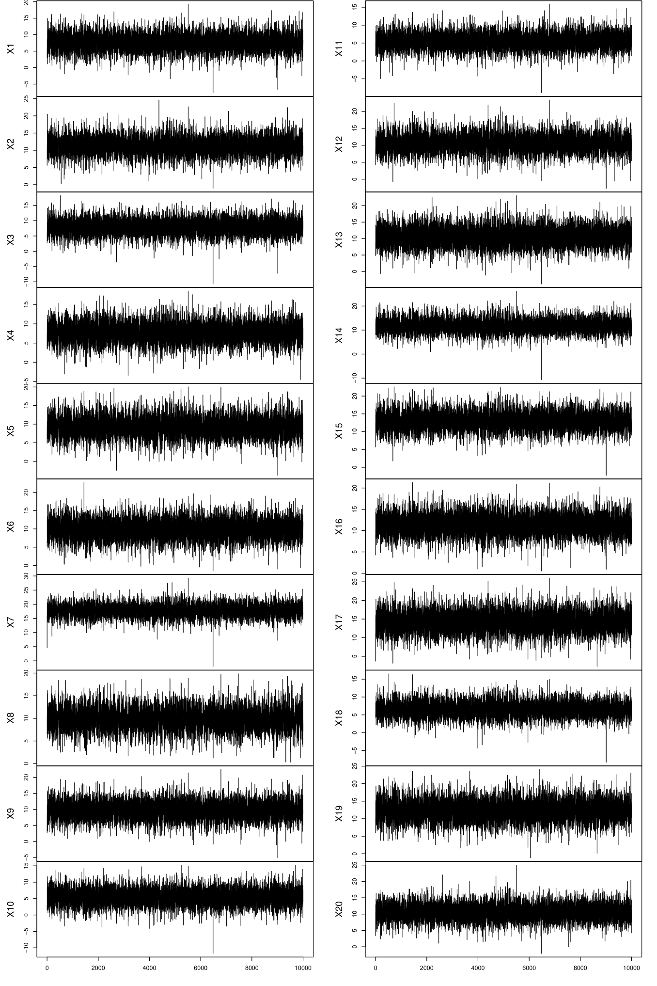
We used the divide-and-conquer approach to estimate the signal dimension with our asymptotic test and the bootstrapping strategy of Matilainen et al. (2018) used in Section 4.1. Additionally, we considered also the ladle estimator using stationary bootstrapping with the expected block length 40. Of each estimator, three versions, AMUSE, SOBI6 and SOBI12, were computed. All nine estimators estimated correctly 3 as the signal dimension and the estimated signals based on SOBI6 are shown in Figure 5.

The computation times of the nine methods were, however, quite different and are given in Table 10.

As all the approaches estimated the dimension correctly, the ones based on the asymptotic test are clearly favourable due to their computational speed. Although, we note that the ladle and the bootstrap tests can also be run parallelized while in the current comparison we used only a single core.

We proposed an asymptotic test for estimating the signal dimension in an SOS-model where the sources include both signal series and white noise. The test does not require the estimation of any parameters and makes quite weak assumptions. This combined with the fact that both of its existing competitors are based on the use of computer-intensive resampling techniques makes the asymptotic test a very attractive option in practice. This conclusion was supported by our simulations studies and real data example exploring dimension estimation for sound recording data.

A central drawback of the proposed method is its inability to recognize non-autocorrelated signals, such as those coming from stochastic volatility models, from white noise. One way to get around this limitation is to replace $\textbf{z}_{2t}$ in (1.1) by a vector of stochastic volatility series and to revert the roles of signal and noise. That is, we use hypothesis testing to estimate the dimension of the “noise” subspace (containing the stochastic volatility components) and separate them from the uninteresting “signal” series exhibiting autocorrelation. For this to work, a limiting result equivalent to Lemma 4 is needed for the above combination model. Similar idea was suggested in the context of the ladle estimator already in Nordhausen and Virta (2018).

Klaus Nordhausen acknowledges support from the CRoNoS COST Action IC1408.

References

- Belouchrani et al. (1997) Belouchrani, A., K. Abed Meraim, J.-F. Cardoso, and E. Moulines (1997). A blind source separation technique based on second order statistics. IEEE Transactions on Signal Processing 45, 434–444.
- Brockwell and Davis (1991) Brockwell, P. and R. Davis (1991). Time Series: Theory and Methods. Springer.
- Chang et al. (2018) Chang, J., B. Guo, and Q. Yao (2018). Principal component analysis for second-order stationary vector time series. To appear in The Annals of Statistics ??, ??–??
- Comon and Jutten (2010) Comon, P. and C. Jutten (2010). Handbook of Blind Source Separation. Independent Component Analysis and Applications. Academic Press.
- Ensor (2013) Ensor, K. B. (2013). Time series factor models. Wiley Interdisciplinary Reviews: Computational Statistics 5(2), 97–104.
- Illner et al. (2015) Illner, K., J. Miettinen, C. Fuchs, S. Taskinen, K. Nordhausen, H. Oja, and F. J. Theis (2015). Model selection using limiting distributions of second-order blind source separation algorithms. Signal Processing 113, 95–103.
- Luo and Li (2016) Luo, W. and B. Li (2016). Combining eigenvalues and variation of eigenvectors for order determination. Biometrika 103, 875–887.
- Matilainen et al. (2018) Matilainen, M., C. Croux, J. Miettinen, K. Nordhausen, H. Oja, S. Taskinen, and J. Virta (2018). tsBSS: Blind Source Separation and Supervised Dimension Reduction for Time Series. R package version 0.5.2.
- Matilainen et al. (2018) Matilainen, M., K. Nordhausen, and J. Virta (2018). On the number of signals in multivariate time series. In Y. Deville, S. Gannot, R. Mason, M. D. Plumbley, and D. Ward (Eds.), International Conference on Latent Variable Analysis and Signal Separation, Cham, pp. 248–258. Springer International Publishing.
- Miettinen et al. (2016) Miettinen, J., K. Illner, K. Nordhausen, H. Oja, S. Taskinen, and F. Theis (2016). Separation of uncorrelated stationary time series using autocovariance matrices. Journal of Time Series Analysis 37, 337–354.
- Miettinen et al. (2012) Miettinen, J., K. Nordhausen, H. Oja, and S. Taskinen (2012). Statistical properties of a blind source separation estimator for stationary time series. Statistics & Probability Letters 82, 1865–1873.
- Miettinen et al. (2014) Miettinen, J., K. Nordhausen, H. Oja, and S. Taskinen (2014). Deflation-based separation of uncorrelated stationary time series. Journal of Multivariate Analysis 123, 214–227.
- Miettinen et al. (2017) Miettinen, J., K. Nordhausen, and S. Taskinen (2017). Blind source separation based on joint diagonalization in R: The packages JADE and BSSasymp. Journal of Statistical Software 76, 1–31.
- Mikosch et al. (2009) Mikosch, T., Kreiß, J.-P., R. Davis, and T. Andersen (2009). Handbook of Financial Time Series. Springer.
- Nordhausen et al. (2017) Nordhausen, K., J.-F. Cardoso, J. Miettinen, H. Oja, E. Ollila, and S. Taskinen (2017). JADE: Blind Source Separation Methods Based on Joint Diagonalization and Some BSS Performance Criteria. R package version 2.0-0.
- Nordhausen et al. (2016) Nordhausen, K., H. Oja, and D. Tyler (2016). Asymptotic and bootstrap tests for subspace dimension. Preprint available as arXiv:1611.04908.
- Nordhausen et al. (2017) Nordhausen, K., H. Oja, D. Tyler, and J. Virta (2017). Asymptotic and bootstrap tests for the dimension of the non-Gaussian subspace. IEEE Signal Processing Letters 24, 887–891.
- Nordhausen and Virta (2018) Nordhausen, K. and J. Virta (2018). Ladle estimator for time series signal dimension. In Proceedings of IEEE Statistical Signal Processing Workshop 2018, IEEE SSP 2018.
- R Core Team (2017) R Core Team (2017). R: A Language and Environment for Statistical Computing. Vienna, Austria: R Foundation for Statistical Computing. R version 3.4.1.
- Serfling (2009) Serfling, R. J. (2009). Approximation Theorems of Mathematical Statistics, Volume 162. John Wiley & Sons.
- Tong et al. (1990) Tong, L., V. Soon, Y. Huang, and R. Liu (1990). AMUSE: A new blind identification algorithm. In Proceedings of IEEE International Symposium on Circuits and Systems, pp. 1784–1787. IEEE.
- Van der Vaart (1998) Van der Vaart, A. W. (1998). Asymptotic Statistics. Cambridge University Press.
- Ye and Weiss (2003) Ye, Z. and R. E. Weiss (2003). Using the bootstrap to select one of a new class of dimension reduction methods. Journal of the American Statistical Association 98, 968–979.
Aalto University, Finland
E-mail: joni.virta@aalto.fi
Vienna University of Technology
E-mail: klaus.nordhausen@tuwien.ac.at