Percolation in a distorted square lattice

$L\times L$ distorted lattice is created by slightly ruffling the sites of a regular $L\times L$ lattice. This has been done systematically by setting a distortion parameter $\alpha$ which denotes the maximum amount of dislocation along $x$ or $y$ axis. Such a lattice can be generated using the following steps:

• •

  Initially an empty square lattice with equidistant nearest neighbors is considered. The lattice constant is set to unity.

• •

  A suitable value for the distortion parameter $\alpha$ is fixed. Since the undistorted distance is set to $1$, $\alpha$ may be varied within the range: $0<\alpha<0.5$.

• •

  A lattice site at position $(i,j)$ is chosen. Two random numbers, $r_{x}$ and $r_{y}$, are generated for $x$ and $y$ direction respectively, in the range $\{-\alpha,\alpha\}$. The position of this site is modified to $(X_{ij},Y_{ij})$, where, $X_{ij}=i+r_{x}$ and $Y_{ij}=j+r_{y}$.

• •

  The above step is repeated for every site of the lattice. A distorted lattice is thereby created.

Two suggestive representations of distorted lattice are shown in figure 1 for two different values of $\alpha$. As shown therein, each site can now be located at any point $(i+r_{x},j+r_{y})$ within a square of length $2\alpha$ with the undistorted position $(i,j)$ at the center of the square. The distance between any two neighboring sites is denoted in general by $\delta$. The minimum and maximum limits of $\delta$ are therefore

and

respectively. Note that for $\alpha>0.5$, the lattice is over-distorted: the squares of possible occupancy of two neighboring sites in figure 1(c) would overlap and the notion of identifying a site with reference to the regular lattice points $(i,j)$ would lose its meaning. We restrict this study from low to moderate $\alpha$.

In usual site percolation, some of the empty sites are occupied randomly corresponding to an occupation probability $p$. In the present model, the following process has been adopted after generating the distorted empty lattice:

• •

  The empty sites of the distorted lattice are occupied randomly as per a given $p$.

• •

  A connection threshold ($d$) is set.

• •

  Distance ($\delta$) between any pair of occupied neighbors is calculated. These two neighbors are considered to be connected if $\delta\leq d$; otherwise, the link is broken.

• •

  The above step is repeated for each pair of occupied neighbors and the clusters are identified accordingly to determine the possibility of percolation.

It is clear from the above scheme that even if two nearest neighbors are occupied, they may not belong to the same cluster. This is the main difference of the present model with usual site percolation. The connectivity of any two occupied neighbors depends on $\delta$ (and therefore, on $\alpha$) and on the value of $d$. Since $\delta_{m}\leq\delta\leq\delta_{M}$, the range of interest for the connection threshold $d$ is also $\delta_{m}\leq d\leq\delta_{M}$. If $d<\delta_{m}$, no cluster formation is possible; whereas, for $d>\delta_{M}$, every occupied neighbor is connected and the case is similar to usual (undistorted) site percolation. However, as we shall see in the next section, when $d\leq 1$, the system suddenly ceases to percolate even for $p=1.0$, making the range $\delta_{m}<d\leq 1$ uneventful.

In this work, the cluster identification and numbering has been done by the well known Hoshen-Kopelman (HK) algorithm [34]. The connectivity criterion ($\delta\leq d$) has been incorporated into the HK algorithm to appropriately reflect the properties of distorted lattice. We emphasize that this is a controlled site percolation model and is clearly distinct from bond percolation (where every site is occupied and bonds are occupied randomly) and site-bond percolation (where both the sites and the bonds between the occupied neighbors are occupied randomly) models.

Let us first study the effect of this distortion on the percolation threshold($p_{c}$). For an undistorted square lattice, this value is known to be $p_{c}\approx 0.592746=p_{cu}$ as the lattice size tends to infinity. It is not hard to realize that $p_{c}$ depends on the relative strengths of $\alpha$ and $d$ in a distorted lattice.

To demonstrate these dependences clearly, we first calculate $p_{c}(\alpha)$ for different fixed values of $d$. Fig. 2(a) shows eight curves, one each for a value of $d$ ranging between $1.0$ and $1.25$. All the curves stay at the value $p_{cu}$ as long as $\alpha$ is low enough, so that $\delta_{M}<d$. For example, the (blue) curve for $d=1.25$ at the bottom (see fig. 2(a)) remains at $p_{cu}$ up to an appreciable value of $\alpha$. This is expected since this situation is similar to undistorted percolation (even if $\alpha$ is non-zero) due to large value of $d$. The maximum distance $\delta_{M}$ between the neighboring points has to exceed the connection threshold $d$ for the manifestation of any effect of distortion. For lesser values of $d$, percolation threshold is affected by less distortion. It may be concluded from these plots that when the connection threshold is held fixed, $p_{c}$ increases with $\alpha$. This means more distortion makes it more difficult for the system to percolate. This result can be attributed to the fact that the average distance between two neighboring points increases with $\alpha$ as $\delta_{min}(\alpha)\approx 1+0.337629\alpha^{2}$. For lower values of the connection threshold ($d=1.05,1.025,1.0125,1.0025$ here), $p_{c}$ reaches very close to $1$ at a certain value of $\alpha$. As $d$ becomes smaller, this situation occurs with smaller $\alpha$. This indicates that all the sites need to be occupied to span the lattice. Moreover, if $\alpha$ is further increased the system is no longer guaranteed to percolate. In fig. 2(a), each $p_{c}$ is calculated by generating $200$ independent representations for specific set of $\alpha$ and $d$. For each value of $d$, $p_{c}$ is shown up to the value of $\alpha$ for which all the $200$ representations percolate. At $d=1.0$, the system ceases to percolate for any non-zero value of $\alpha$. We have also checked that this situation persists for any $d<1.0$. Thus, for any value of connection threshold which is less than or equal to the lattice constant (or, the undistorted nearest neighbor distance, here taken to be $1.0$), the system can not percolate if any distortion, be it very small, is present.

This is an important observation in the context of realistic applications of percolation, particularly since a perfectly ordered natural system can hardly be found. Consider, for example the simulation of the forest-fire model. Here, $d$ can be interpreted as the fire-spreading threshold. A distorted array will make it difficult for the fire to percolate. Moreover, depending on the relative values of $\alpha$ and $d$, distortion can even completely stop fire-percolation in a forest where the fire would have definitely percolated for an undistorted array of same number of trees.

Variation of the percolation threshold($p_{c}$) with the connection threshold($d$) is shown in fig. 2(b) for six different values of the distortion parameter ($\alpha$). A higher value of $d$ is expected to favor percolation and this is evident from fig. 2(b), which shows that $p_{c}$ decreases with $d$ when $\alpha$ remains fixed. If $d$ is large enough (and $\alpha$ is small enough) to ensure that $d>\delta_{M}$, the effect of distortion disappears and consequently, the percolation threshold stays at $p_{c}=p_{cu}$. In the other extreme, spanning becomes more difficult with a low connection threshold and beyond a certain value, system can not percolate even after occupying all the sites. For each $\alpha$, the displayed data start with the minimum value of $d$ which ensures that all the $200$ independent realizations do necessarily percolate.

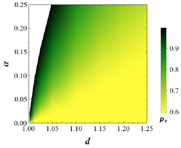
All the plots of fig.2(a) and fig.2(b) can be regarded as separation curves between percolating and non-percolating phases. This is shown in fig.3. For example, if $d=1.025$ and $\alpha=0.05$, spanning is guaranteed if $85\%$ of the sites are occupied, since the point ($0.05,0.85$) in fig.3(a) falls in the percolating (green) region. Similarly, if $\alpha=0.15$ and $d=1.05$, a $70\%$ occupancy is not sufficient for spanning (see fig.3(b)).

The density plot (fig.3(c)) shows the variation of the percolation threshold with both connection threshold and distortion. Higher $p_{c}$ is obtained for high $\alpha$ and low $d$. The blank portion on the left side indicates that the system can not percolate for those values $\alpha$ and $d$.

The percolation order parameter is usually defined as

where $S_{max}$ stands for the number of occupied sites in the largest cluster and $\langle\rangle$ denotes configuration-average. In order to calculate $\Omega_{L}(p)$ for an $L\times L$ system , one needs to occupy the sites as per the occupation probability $p$, count the number of sites in the largest cluster, average over many such configurations and finally divide it by $L^{2}$. In fig. 4(a), $\Omega_{L}(p)$ is plotted for four values of the distortion parameter $\alpha=0,0.1,0.15,0.2$ from left to right for a fixed $d=1.1$. As the effect of distortion diminishes, the curve shifts towards left. Similar situation is displayed in fig. 4(b); here the influence of distortion is reduced by increment in connection threshold ($d$), although $\alpha=0.1$ remains unchanged. In fig. 4(b), the two curves on the left are very close to each other. This indicates that the undistorted scenario is being approached and the curves with still higher $d$ would be identical.

Figure 5(a) shows $\Omega_{L}(p)$ for different system sizes: $L=128,256,512,1024$, with the steepest one corresponding to the largest $L$. The parameters of $\alpha=0.2$ and $d=1.1$ have been held fixed. For this set of values we find $p_{c}=0.8025$. Using the value of the critical exponent $\nu=0.75$ for standard percolation, when the horizontal axis is scaled as $(p-p_{c})L^{1/\nu}$, the curves of $\Omega_{L}(p)$ separate from each other with the $L=128$ curve being on top and the $L=1024$ one at the bottom. The values of $\Omega_{L}(p)$ are collected at a fixed value of $(p-p_{c})L^{1/\nu}$ and using these values a plot of $\ln\Omega_{L}(p)$ with $\ln L$ is generated (see inset of figure 5(a)). The slope of the straight line fit of this data gives $\beta/\nu=0.1143$. As known from standard percolation criticality, if the vertical axis is now scaled as $\Omega_{L}(p)L^{\beta/\nu}$ and plotted against $(p-p_{c})L^{1/\nu}$, a data collapse should be obtained. We do get a nice data collapse in figure 5(b) using the obtained value of $\beta/\nu$.

It is known that the percolating cluster at $p=p_{c}$ is a fractal whose fractal-dimension $d_{f}$ is given by

We calculate $\langle S_{max}\rangle$ for $L=2^{7},2^{8},2^{9},2^{10}$ with $\alpha=0.2$ and $d=1.1$ at $p=0.8025=p_{c}$. Eq. 4 suggests that a log-log plot of $\langle S_{max}\rangle$ and $L$ would fit into a straight line with its slope$=d_{f}$. In the inset of figure 5(b), we show this plot along with a linear fit that gives $d_{f}=1.8857$. This confirms the well known relation between the fractal dimension of the percolating cluster at $p_{c}$ and the relevant critical exponents in two dimensional systems

The whole process has been repeated for two other sets of values of $\alpha$ and $d$ (plots are not shown as they look very similar to those given in figure 5). For $\alpha=0.1,d=1.1$, we get $p_{c}=0.6617,\beta/\nu=0.1150$ and for $\alpha=0.2,d=1.2$, we get $p_{c}=0.6665,\beta/\nu=0.1165$. These values should be compared to those for the ordinary percolation, for which, $\beta/\nu=0.1012$ and $d_{f}=1.8958$.

These results tend to indicate that the present variant of percolation in a distorted lattice may belong to the same universality class as the ordinary percolation. It has to be understood that within the scope of the present work, the values of the exponents, percolation threshold and fractal dimension are suggestive. More precise values, rigorous analysis on their dependence on $\alpha$ and $d$ and a conclusive decision on universality class require further detailed study and extensive numerical calculation involving averages over larger number of configurations with (preferably) bigger lattice sizes. We plan for such a detailed study in our future endeavor.