Quantum Rabi Model with Two-Photon Relaxation
Abstract
We study a cavity-QED setup consisting of a two-level system coupled to a single cavity mode with two-photon relaxation. The system dynamics is modeled via a Lindblad master equation consisting of the Rabi Hamiltonian and a two-photon dissipator. We show that an even-photon relaxation preserves the symmetry of the Rabi model, and provide a framework to study the corresponding non-Hermitian dynamics in the number-parity basis. We discuss the role of different terms in the two-photon dissipator and show how one can extend existing results for the closed Rabi spectrum to the open case. Furthermore, we characterize the role of the symmetry in the excitation-relaxation dynamics of the system as a function of light-matter coupling. Importantly, we observe that initial states with even-odd parity manifest qualitatively distinct transient and steady state behaviors, contrary to the Hermitian dynamics that is only sensitive to whether the initial state is parity-invariant. Moreover, the parity-sensitive dynamical behavior is not a creature of ultrastrong coupling and is present even at weak coupling values.
Introduction. The Rabi model [1] describes the quantum interaction between a two-level system (TLS) and a bosonic mode. Despite its simple form, the Rabi model represents an important theoretical building block of quantized matter-field interactions and quantum information processing. It is applicable to a broad range of quantum phenomena spanning microscopic to mesoscopic systems, finding realizations in a wide range of quantum platforms, including cavity-QED [2, 3, 4, 5], circuit-QED [6, 7, 8, 9, 10, 11], nanoelectromechanical [12, 13, 14, 15], quantum-dot [16], and trapped-ion [17, 18] systems.
Light-matter interactions within the Rabi model consist of rotating (resonant) and counter-rotating (non-resonant) contributions. Traditionally, Rabi dynamics is analyzed under the rotating-wave approximation (RWA), resulting in the simplified Jaynes-Cummings (JC) model [19], valid when the coupling constant is much weaker than the TLS and mode frequencies. From the perspective of symmetry, RWA fictitiously extends the symmetry of the model to a symmetry, making the total excitation number the second conserved quantity besides the Hamiltonian and therefore facilitates analytical solutions. The JC model has been employed successfully to describe the dynamics of most cavity-QED setups [2, 3, 4, 5]. However, with the advent of superconducting quantum devices, it has become feasible to reach ultrastrong [20, 21] and, more recently, deep-strong [22] regimes of interactions. The breakdown of RWA in these regimes motivated various theoretical efforts to revise the Rabi model. First, generalized versions of RWA [23, 24] were introduced that captures correctly stronger couplings. Second, despite the contemporary understanding, Braak [25] argued that the symmetry of the Rabi model is sufficient for its integrability, showing that the regular spectrum in each parity subspace can be obtained from the roots of a transcendental function. Moreover, Chen et al. provided a more physical derivation of the Rabi spectrum using Bugoliubov transformations [26], contrary to the Bargmann representation [27] employed by Braak. These early studies paved the way toward ongoing developments of analytical and perturbative methods for determining the spectrum, eigenmodes, and dynamics of the Rabi model under different parameter regimes [28, 29, 30, 31, 32].
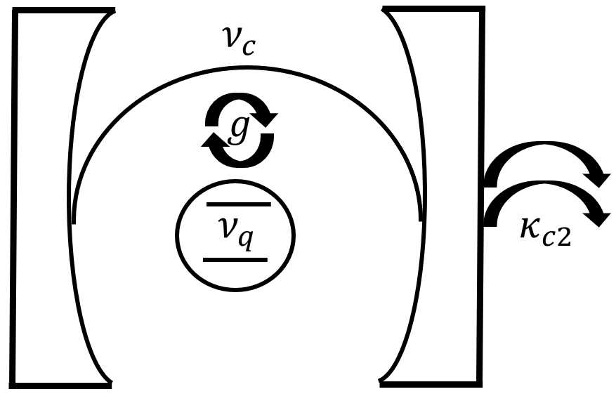
To date, however, most works have focused primarily on ideal, closed (Hermitian) properties of the Rabi model, while role of symmetry in realistic, open (non-Hermitian) scenarios remains an open question. An even exchange of excitations between a cavity mode and environment conserves the symmetry. The latter is particularly important given emerging studies of the dynamics of a single cavity mode under two-photon relaxation [35, 36, 37, 38, 39, 40, 41, 42]. Such a relaxation process has been recently implemented in circuit-QED [34] following a four-wave mixing scheme proposed first by Wolinsky and Carmichael [33] (see SM 11 1 The supplementary material provides further discussion on physical realization of two-photon relaxation, symmetry of the Rabi model and comparison between phenomenological and full spectrum. It includes the following references: [33, 34, 55, 48, 51, 56, 57]). A major motivation behind recent studies of even-photon relaxation processes is their application to realization of dynamically protected, universal quantum computing paradigms [44, 45, 46, 47], in which the quantum information is encoded in logical qubits consisting of Schrödinger cat states with distinct parity that exhibit reliable protection to photon dephasing and single-photon relaxation errors [44].
In this Letter, we generalize the theory of symmetry of the Rabi model to the open quantum case. We first review the spectrum of the closed Rabi Hamiltonian, providing analytical recursion relations for both the eigenfrequency and eigenmodes of the system. Our analysis and calculation are performed in the (cavity) number-(overall) parity representation [48], where the symmetry of the model is explicit. For the open scenario, we consider a Lindblad master equation [49, 50] of the Rabi Hamiltonian with two-photon dissipation for the cavity mode. To analyze its spectral properties, we employ an effective Hamiltonian obtained by keeping diagonal decay terms, while neglecting the off-diagonal collapse in the two-photon dissipator. This phenomenological treatment provides a reliable approximation to the complex eigenfrequencies, but not necessarily the eigenmodes and ground state. While an exact definition of a full effective Hamiltonian exists, mapping the Lindblad dynamics into a norm-preserving Schrodinger equation [51], analytical treatment of its associated spectrum seems prohibitive due to its significantly larger Hilbert space compared to the phenomenological model (see SM for comparison). We follow numerical integration of the Lindblad equation for studying the dynamics, while the effective phenomenological Hamiltonian is primarily used for approximate analytical discussion of the spectrum and a better understanding of the observed dynamics.
Model. Our system consists of a TLS coupled to a single cavity mode, engineered such that single-photon is negligible compared to two-photon relaxation, constraining it to exchange only pairs of photons with the environment (Fig. 1). We model the system dynamics via the Linbdlad equation
| (1a) | ||||
| (1b) | ||||
with , , and denoting the qubit frequency, cavity frequency, and light-matter coupling, respectively. Two-photon relaxation is described via the dissipator, , with denoting the two-photon relaxation rate.
We next transform the Lindblad Eq. (1a) such that the symmetry of the Rabi Hamiltonian and two-photon relaxation become explicit (see SM). In particular, we define the overall parity operator for the system as
| (2) |
The symmetry of the Rabi Hamiltonian (1b) means that . Consequently, the Hilbert space can be partitioned into parity subspaces having even (plus) and odd (minus) total excitation numbers:
| (3a) | ||||
| (3b) | ||||
The adjacent states in each subspace are coupled via both rotating or the counter-rotating terms. If we neglect the latter, each subspace is reduced into a collection of number-conserving Jaynes-Cummings doublets , given by:
| (4a) | ||||
| (4b) | ||||
| number-excitation basis | ||
|---|---|---|
| number-parity basis |
Defining a new set of bosonic operators, , and replacing in terms of the parity operator of Eq. (2), one can rewrite the Rabi Hamiltonian (1b) as [48]
| (5) |
The parity and bosonic operators commute, and thus provide a complete basis for the Hilbert space defined as and for and , respectively. Table 1 summarizes the correspondence between the (old) number-excitation and (new) number-parity bases.
Next, we rewrite the original Lindblad Eq. (1a) in this basis, starting by observing that the two-photon dissipator is also invariant under the parity transformation, i.e. , where also implies that . In the quantum treatment of dissipation, the two contributions to the dissipator are described by decay and collapse terms. The former represents the rate at which a quantum state loses probability while the latter represents the rate at which lower states in the excitation ladder receive probability, in such a way that the net probability is conserved in time, i.e. . Separating the two contributions, one can reexpress the Lindblad Eq. (1a) to yield,
| (6a) | |||
| with denoting the phenomenological effective Hamiltonian as | |||
| (6b) | |||
Neglecting the coupling induced by collapse, the last term in Eq. (6a), the dissipative dynamics is approximated by . This framework is a middle ground in which the unitary part of the system dynamics is treated quantum mechanically, while the dissipation is treated phenomenologically. Essentially, such an approach provides a good approximation for the complex spectrum of the problem, while ignoring proper characterization of the modal and ground state information (See Sec. IV of the SM for further discussion).
Spectrum. Here, we first revisit the spectrum of the closed Rabi model and benchmark our solution against those of Braak [25]. For the open case, we study the impact of two-photon relaxation via of Eq. (6b). In particular, we show that the typical solution obtained for the closed case can be generalized to yield the complex eigenfrequencies of the open system.
We begin with the eigenvalue problem for the closed Rabi model, , where labels the eigenvalues and eigenmodes at a nonzero and is the corresponding parity subspace. Expanding the unknown eigenmodes in terms of the number-parity basis, , one finds that the eigenfrequencies are obtained by the roots , where and satisfies the following recursion relation (see SM):
| (7) |
subject to initial conditions, and . The coefficients in the recursion Eq. (7) read
| (8) | ||||
Similarly, the corresponding eigenmodes are determined by yet another recursion relation for the probability amplitudes , given by:
| (9) | ||||
with initial conditions, . An illustrative example of the variation of the spectrum with respect to is shown in Fig. (2a), with parameters chosen to compare our results with those in Fig. 2 of Ref. [25].
Within the phenomenological treatment of relaxation, the system dynamics are determined by of Eq. (6b). Here, we find that the recursion relations determining the eigenfrequencies (7) and eigenmodes (9) have the same form as those of the closed system, except that the coefficients are modified as (see SM). To understand the changes induced by phenomenological decay (compared to the closed), we first consider the regime of zero coupling , where the decay terms are diagonal in the number basis. In this scenario, the th bare cavity mode acquires a decay rate of , resulting in nonzero values for all cavity number states except the ground and first-excited state, for each parity. As the coupling is turned on, the hybridization between the qubit and the cavity mode allows these terms not only to induce additional decay, but also modify the real frequency of each state. Figure 2 (dotted lines) shows such hybridization as a function of , as calculated by the phenomenological model. We note that an analogous phenomenological model based on the JC model can be solved analytically and result in decay rates that plateau at ultrastrong coupling values of and hence mischaracterizes the interplay of light-matter coupling and two-photon relaxation (see SM for comparison).
Excitation-relaxation dynamics. Here, we study the dissipative dynamics of the system and discuss the role of symmetry. For concreteness, we consider the situation in which the cavity is initially prepared with an even or odd number of photons, and describe the ensuing dynamics of the cavity photon and qubit population as a function of both time and . In particular, we consider two scenarios of starting with two [] or three [] initial cavity photons and the qubit in ground state, as representatives of the plus or minus parity subspaces. Due to pair-exchange of photons with the environment, we intuitively expect states with even or odd initial cavity photons to exhibit different transient and steady state behavior.
First, consider the simplest case of . This choice of parameter decouples the qubit and hence corresponds to the problem of a single cavity mode with two-photon relaxation, which has been studied in detail using multiple methods [38, 39, 40, 41, 42]. In this case, initial states having even (odd) numbers of cavity photons end up with zero (one) cavity photons in the steady state 22 2 Note that states with mixed parity can always be expressed as linear combinations of two independent problems..


Next, we move on to characterize the interplay of two-photon relaxation and the qubit for . Here, closed form analytical solutions of the evolution operator at arbitrary seem intractable, and instead we employ numerical integration of the Lindblad Eq. (6a). The time evolution of the cavity/qubit excitations as a function of is studied in Figs. 3 and 4 for the cases of two and three initial cavity photons, correspondingly. In both cases, it is generally observed that as is increased, more complex beatings between various normal modes emerge. Such beatings can be approximately understood from the mapping of the initial cavity state to the corresponding eigenmodes of the open Rabi model. This shows which modes are more active at a given value of in each parity subspace (Figs. 3c and 4c). For example, for the case of , the initial probability is shared between states and up to intermediate values of g (), beyond which and dominate. The corresponding frequency and decay rate of the modes can be obtained from Figs. 2a-2b.
Despite this generic similarity, it is observed that due to the nontrivial interplay of light-matter coupling and two-photon relaxation, the two cases under consideration have different transient and steady state characteristics. For the case of two initial cavity photons, we observe that the system reaches steady state on a timescale that is more or less given by the two-photon relaxation rate (Figs. 3a-3b). On the other hand, in the case of three initial cavity photons, the transient dynamics has more features. Generally, at small , the dynamics can be described as follows (Figs. 4a-4b): First, a fast depletion of the initial three cavity photons into one photon, with timescale roughly determined by . This can be seen by the sharp transition of the cavity excitation number from 3 to approximately 1 (red to blue in Fig. 4a). Second, a slower depletion of the remaining cavity photon after a large number of Rabi exchanges between the qubit and the cavity, with timescale roughly determined by the decay rate of state . Essentially, since two-photon relaxation only allows pairs of exchange with the environment, the quantum state acts like a dark state at (i.e. ). As is increased, the decay rate of this state is barely modified up until (See Fig. 2b), consistent with the observed long-lived excitations in the qubit and cavity dynamics (Figs. 4a-4b).
Steady state excitations have also been studied as a function of in Figs. (3d-4d). In the case of two initial photons, we observe that the steady state populations of the cavity and qubit increase non-monotonically with increasing , exhibiting a local maximum close to . The case of three initial photons is more complicated. For small , one observes fast relaxation of two photons, while the remaining photon energy is transferred to the qubit at steady state. At intermediate values of , the excitation is shared between the cavity and the qubit while at very large , the qubit excitation saturates and the cavity photon population increases linearly (Fig. 4d). The overall increase observed in the steady state populations arises from the fact that the coupling in Eq. (6b) appears effectively as an incoherent drive on the cavity. Lastly, we note that the steady state quantities obtained from the Linbdlad formalism will become less accurate at large values of , as one needs to account for the renormalization of the dissipator arising from the underlying system-bath formalism [53], resulting in a Bloch-Redfield master equation [54]. Using Rayleigh-Schrödinger perturbation theory, however, one can show that disspator renormalizations are higher order in compared to the ones for the Hamiltonian. This leaves a window, at intermediate values of coupling, where the use of bare dissipators is still justified.
Acknowledgements. We appreciate helpful discussions with Pengning Chao. This work was supported by the National Science Foundation under Grant No. DMR-1454836, Grant No. DMR 1420541, and Award EFMA-1640986.
Supplementary material: Quantum Rabi model with two-photon relaxation
The structure of this supplemental material section is as follows. We first revisit a possible physical realization of two-photon relaxation for a cavity in Sec. A. The symmetry of the Rabi model is discussed in detail in Sec. B. In Sec. C, we first revisit the spectrum of the closed Rabi model in its parity representation and extend the result to the open case up to phenomenological treatment of the opening. Section D provides further discussion on the validity of the phenomenological treatment and its comparison with the full spectrum.
Appendix A Physical realization of two-photon relaxation
In this section, we discuss potential physical realization of two-photon relaxation. In order to achieve a dissipator of the form for the cavity, in principle, one needs to engineer a cavity-bath coupling of the form
| (10) |
where denotes the strength of the two-photon coupling between the cavity mode and mode of the bath. Such a coupling requires a three-wave mixing in which two cavity photons convert into one bath photon, but in practice, it is realized by means of four-wave mixing including an additional pump tone. In what follows, we revisit the proposal by Wolinsky and Carmichael [33], which have been recently experimentally implemented in the context of superconducting circuits [34].
In this scheme, the original cavity is required to have a very high quality factor in order to suppress the single-photon relaxation rate. The dominant two-photon relaxation is then achieved by engineering a quartic Kerr coupling to an additional linear cavity as shown in Fig. 5. In superconducting circuits, the quartic nonlinearity can be realized via a weakly nonlinear Josephson junction, in which the cosine potential can be well approximated by the lowest order quartic interaction. The auxiliary readout cavity, on the contrary, has to have very low quality factor in order to quickly dissipate the converted cavity photon pairs into the environment without significant back-scattering.
To achieve the desired conversion, the frequencies of the pump and the cavities should satisfy the frequency matching condition
| (11) |
Under condition (11), the Hamiltonian for the overall system shown in Fig. 5 can be approximated up to rotating-wave approximation as [34]
| (12) | ||||
where denotes the annihilation operator of the readout cavity. Importantly, in this scheme, we have achieved a pump-induced two-photon coupling as with being the coherent amplitude of the readout cavity and the corresponding single-photon rate. The second line of Eq. (12) keeps track of the additional self- and cross-Kerr interactions denoted by , and and can be considered as smaller perturbation compared to . The additional drive tone at the readout frequency and amplitude is responsible to prepare the readout cavity with approximately one photon in order to fine-tune the desired conversion. Integrating out the readout degrees of freedom will result in an effective two-photon dissipator for the cavity as with relaxation rate given as [34]
| (13) |
Finally, we note that in contrast to the aforementioned active implementation that employs two drive tones, it might be also feasible to achieve a passive implementation following similar ideas as the circuit-QED proposal by Felicetti et. al [55] that is capable of achieving two-photon quantum Rabi model using a phase qubit coupled to a DC-SQUID.

Appendix B symmetry of the Rabi model
In this section, we revisit the symmetry of the Rabi model and discuss the transformation that diagonalizes the Hamiltonian in its parity representation.
We start with the Rabi Hamiltonian,
| (14) |
where and are the cavity and qubit bare frequencies and represents the light–matter coupling strength. We define the overall parity operator by its action on the spin and photonic degrees of freedom:
| (15) |
From (15), one can derive the standard properties of a parity operator, including involution , unitarity , and Hermiticity . The overall parity operator can then be written as a product of the spin and photonic parity operators as
| (16) |
The symmetry of the Rabi Hamiltonian (14) means that remains invariant under the transformation
| (17) |
In the following, we rewrite the Rabi Hamiltonian such that the symmetry becomes explicit. In particular, we introduce the following new set of bosonic creation and annihilation operators,
| (18) |
from which it follows that,
| (19a) | ||||
| (19b) | ||||
Employing Eqs. (16) and (19b), one can rewrite the Rabi Hamiltonian (14) as [48]
| (20) |
Since the parity and number operators commute, their eigenstates provide a complete basis for the Hilbert space of the problem. Hence, we define the number-parity basis , which satisfies:
| (21a) | ||||
| (21b) | ||||
The advantage of working with the transformed Rabi Hamiltonian (20) is that it is explicitly block-diagonal in the parity sector,
| (22) |
with denoting the Hamiltonians of the even () and odd () parity subspaces, given by:
| (23) |
Appendix C Spectrum of the Rabi model
In this section, we study the spectrum of the Rabi Hamiltonian (23) and show that the results can be extended to account for the open case up to phenomenological treatment. At last, we provide a comparison to the open JC, in which the counter-rotating terms in the coupling are dropped. We begin by considering the eigenvalue problem for each parity subspace,
| (24) |
where and denote the eigenfrequency and eigenmode for each parity , respectively.
Expanding the unknown wavefunctions in terms of the number-parity basis,
| (25) |
and inserting this expansion into the eigenvalue problem (24), one obtains
| (26) | ||||
Reindexing the sums and employing the linear independence of the number-parity basis , we obtain the recurrence relation for as
| (27a) | ||||
| with , and defined as | ||||
| (27b) | ||||
| (27c) | ||||
| (27d) | ||||
| and with initial conditions, | ||||
| (27e) | ||||
The recursion relation (27a) and the associated initial condition (27e) uniquely determine in terms of for arbitrary .
Next, we need to obtain an equation to determine the eigenfrequencies . Note that the recursion relation above can be represented in matrix form, , in terms of the infinite-dimensional tridiagonal matrix:
| (28) |
Hence, the roots of the determinant of yield the eigenfrequencies corresponding to subspace . Denoting the determinant , where is an truncation of , and employing a Laplace expansion, one can obtain a recursive relation for the determinant,
| (29) |
with initial condition and . Defining,
| (30) |
it follows that the th eigenfrequency in each subspace is given by the th root of , obtained by solving . The corresponding eigenmode is found by replacing in Eq. (27b) to find and related quantities accordingly.
If the relaxation is accounted phenomenologically, we employ the effective Hamilatonian as
| (31) |
Note that the additional term is diagonal in the number basis with matrix elements . Therefore, following the same steps as in Eqs. (25-26), we find similar recursion relations as Eqs. (27a) and (29), for the eigenmodes and spectrum respectively, where the diagonal coefficient gets replaced due to the dissipative contribution as
| (32) | ||||
while the off-diagonoal coefficients and remain intact. As expected, the eigenfrequencies become complex. An example comparing the closed and open spectrum is shown in Fig. 2 of the paper.
Lastly, we study the Jaynes-Cummings (JC) model with two-photon relaxation and employ the analytical solutions to its spectrum to compare to and benchmark the result obtained from our recursion relations. Consider the phenomenological effective JC Hamiltonian with two-photon relaxation [analogous to Eq. (31)] as
| (33) |
where the counter-rotating terms are dropped. Hamiltonian (33) commutes with the total excitation number . Therefore, it is block-diagonal consisting of the singlet with eigenfrequency and doublets as
| (34) |
The eigenfrequencies of Eq. (34) can be immediately found as
| (35a) | ||||
| (35b) | ||||
where the labels are chosen to be consistent with our convention for the Rabi eigenvectors . Figure 6 provides a comparison between the phenomenological spectrum obtained from the Rabi and JC models. Besides the well-known spurious level crossings that is observed in the real part of the JC spectrum (Fig. 6a), we observe that the JC model generate decay rates that plateau as is enhanced and hence completely mischaracterizes the interplay of the coupling and the two-photon relaxation at ultrastrong coupling (Fig. 6b).
Appendix D Full effective Hamiltonian
In the previous section, we obtained a rather simple generalization of the recursion relation for the spectrum to the open case up to phenomenological treatment of the opening [Eq. (32)]. We have employed the resulting approximate result to analyze the excitation-relaxation dynamics discussed in the main paper. The main purpose of this section is to provide more discussion on the validity of such an approximation. In subsection D.1, we first revisit the possibility of extending the effective Hamiltonian approach such that it accounts for the collapse terms as well. The full effective Hamiltonian belongs to a larger Hilbert space, hence an immediate question is the possibility of decomposition of the full spectrum. This is discussed in subsection D.2. Subsection D.3 applies the full effective Hamiltonian approach and the spectral decomposition on the simplest case of a two-level system with relaxation, and provides important insight on the role of collapse term in renormalizaiton of eigenmodes and spectrum. Finally, in Sec. D.4, we provide a comparison between the spectrum derived from phenomenological and full effective Hamiltonian approaches for our system.
D.1 General discussion
Here, we revisit the derivation of the full effective Hamiltonian approach for open quantum systems that was first introduced by Yi et. al [51]. Consider a generic Lindblad equation
| (36a) | |||
| where and are the system density matrix and Hamiltonian, respectively. Moreover, we assume a set of dissipation channels, with relaxation rate and collapse operator of the form | |||
| (36b) | |||
The diagonal terms (anti-commutator) in Eq. (36b) can be expressed as effective decay if we define an effective system Hamiltonian as
| (37a) | |||
| in terms of which the original Lindblad Eq. (36a) can be recast into | |||
| (37b) | |||
The idea of the full effective Hamiltonian approach is to map the Lindblad Eq. (37b) to an effective Schrodinger equation. This is achieved by introducing an auxiliary system with the same Hilbert space size as the original system, which plays the role of adjoint (left) quantum states. This allows extending the size of the composite Hilbert space to that of the original Lindbladian. We therefore introduce a full orthonormal basis and define the following full wavefunction
| (38) |
where are the matrix elements of the system density matrix defined as . We then seek an effective Hamiltonian such that the Schrödinger dynamics of the pure wavefunction matches the original Lindblad dynamics in terms of the matrix elements .
The resulting full effective Hamiltonian for the system can be found as [51]
| (39a) | ||||
| where and are the effective Hamiltonian and collapse operator for the auxiliary system that satisfy | ||||
| (39b) | ||||
| (39c) | ||||
Consequently, in this approach, we seek a solution to the wavefunction as
| (40) |
from which one can infer the solution for .
Equation (39a) clarifies the distinction between the phenomenological effective Hamiltonian (37a) and the full effective Hamiltonian more clear. In the phenomenological treatment, the system spectrum is determined by the eigenvalues of , where the additional coupling caused by the collapse operators between the left and right states are neglected.
D.2 Spectral decomposition
At first sight, it seems that the additional coupling (last term) in the full effective Hamitlonian (39a) breaks the possibility of spectral decomposition, i.e. writing the full spectrum as linear sum of each constituent. It has been shown that for quadratic Lindbladians it is feasible to obtain a reduced effective spectrum for the system in terms of the full spectrum [56] due to the following self-conjugation symmetry. Note that under the transformation
| (41a) | |||
| which maps the original system to the adjoint system, we obtain from Eq. (39a) the self-conjugation symmetry | |||
| (41b) | |||
The consequence of symmetry (41b) for a quadratic Lindbladian is that the full eigenfrequencies can always be effectively decomposed as
| (42) |
where is the set of full eigenfrequencies and is the set of reduced eigenfrequencies for the system that accounts for the collapse terms by construct. Assuming that we have access to the full spectrum, analytically or numerically, we face the problem of obtaining reduced complex eigenfrequencies for the system in terms of the corresponding full complex eigenfrequencies, with being the cut-off number for the Hilbert space.
We note that the elementwise Eq. (42) can be compactly represented as a Tensor Rank Decomposition [57] problem of the form
| (43a) | ||||
| or in terms of real frequency and decay rate tensors as | ||||
| (43b) | ||||
| (43c) | ||||
with , , being the identity, frequency and decay matrices for each sector. The solution for in terms of is unique up to a overall translation, e.g. if is a solution then is also a solution for . This is not an issue, since the overall constant only changes the global reference point with respect to which the frequency levels in are evaluated, while leaves the physical difference that appears in the time-evolution of the system invariant.
In contrast to the spectrum, it is not in general possible to tensor decompose the full eigenmodes into a reduced set of eigenmodes for the system. As an example, a full quantum state
| (44) |
is a valid possibility for the full eigenmode since it respects the symmetry (41b) of the full Hamiltonian. However, a full quantum state like Eq. (44) can not be expresed as a tensor product of two independent states in each sector, i.e. .
D.3 A two-level system with relaxation
Here, we study the case of a two-level system with relaxation. The aim of this subsection is to apply the tools from Secs. D.1 and D.2 on a rather simple example that can be handled analytically. The main outcome of this calculation is that the phenomenological treatment of the opening captures the spectrum correctly, but not the ground state and the modal structure in general. Hence, using the phenomenological treatment provides a good approximation of the spectrum (in this case exact), but cannot be used to draw conclusions about the eigenmodes and in particular the steady state.
Consider the Lindblad equation
| (45) |
where and are the Hamiltonian and the dissipator superoperator given in terms of spin- Pauli matrices as
| (46) | ||||
| (47) |
In terms of the phenomenological effective Hamiltonian
| (48) |
with complex frequency , we can reexpress Eq. (45) as
| (49) |
Next, we discuss the solution to the Lindblad Eq. (49) using Effective Hamiltonian approach. The full effective Hamiltonian includes an auxiliary TLS and reads
| (50) |
where we have denoted the spin operators of the auxiliary system with . In the following we prepare the system in a generic pure state
| (51) | ||||
and solve for the Schrodinger equation
| (52) |
Expressing the full effective Hamiltonian (50) in the basis we find
| (53) |
We can then directly compute the matrix representation of time-evolution operator as
| (54) |
The solution for is obtained as
| (55) |
which can be expressed element-wise as
| (56a) | ||||
| (56b) | ||||
| (56c) | ||||
| (56d) | ||||
It is instructive to clarify the role of collapse term in this rather simple example. The full effective Hamiltonian (53) is lower triangular, i.e. that the collapse term does not change the eigenfrequencies, but rather the eigenvectors of the system. Regardless of the inclusion of the collapse terms, the eigenvalues of read
| (57a) | ||||
| (57b) | ||||
| (57c) | ||||
| (57d) | ||||
On the other hand, if the collapse term is neglected, the eigenvectors are simply the starting excitation basis ; while the eigenvectors of Eq. (53) read
| (58a) | ||||
| (58b) | ||||
| (58c) | ||||
| (58d) | ||||
Therefore, the last eigenvector changes from to . The modification of the eigenvector has a significant impact on the dynamics and the steady state in particular. For example, without the collapse term, the solution for in Eq. (56d) is wrongly reduced to , which breaks the conservation of probability.
D.4 Rabi model with two-photon relaxation
In this subsection, we discuss the derivation of the full effective Hamiltonian approach for the quantum Rabi model with two-photon relaxation and check the validity of the phenomenological results for the spectrum. We start by the Lindblad equation
| (60) |
where we have included a two-photon relaxation for the cavity mode.
Importantly, the two-photon dissipator respects the symmetry of the Rabi model, since
| (61) |
Therefore, we expect that the full Lindblad equation become block-diagonal in the parity sector. To see this explicitly, we first divide the dissipator into decay and collapse contributions and rewrite the Lindblad Eq. (60) as
| (62) |
where the effective system Hamiltonian reads
| (63) |
Second, we reexpress the Lindblad Eq. (62) in the number-parity basis. Using definition (18) we find that
| (64) |
from which we can reexpress the effective system Hamiltonian (63) as
| (65) |
The Lindblad Eq. (62) then takes the form
| (66) |
Comparing Eq. (66) to the generic Lindblad form (37b) and following the discussion in Sec. (D.1), we can define a full effective Hamiltonian as
| (67a) | ||||
| where and are defined as | ||||
| (67b) | ||||
| (67c) | ||||
In Eqs. (67a-67c), and denote the cavity annihilation and parity operators for the system sector, while and are the counterparts for the auxiliary sector.
Even though it is in principle possible to obtain recursion relations for the eigenfrequencies and eigenmodes of the full effective Hamiltonian (67a), due to the larger Hilbert space compared to the phenomenological treatment, the results will be more involved. Alternatively, we avoid analytics and compute the complex spectrum of the full effective Hamiltonian (67a) numerically.
To make a meaningful comparison to the phenomenological result of Sec. C, we can in principle follow two possible routes. The first possibility is to employ spectral decomposition of the full spectrum, which provides a reduced spectrum that could be in principle compared with the phenomenological result. The Rabi model is not quadratic, and a numerical study shows that the aforementioned spectral decomposition [Eq. (43a)] does not hold for this system. Therefore, we follow the second possibility of using the Hamiltonian , that lacks the collapse terms, and compare its spectrum with that of in Eq. (67a). An example for the spectrum is shown in Figs. 7 and 8 for the real part (frequency) and imaginary part (decay) of the complex spectrum, respectively. For clarity, the spectrum has been partitioned into four (i.e. ) possible parity subspaces. Following the results in the main paper, we have kept the lowest 5 levels for the system and auxiliary bosons. Therefore, we observe distinct quantum levels for each of the four possible parity subspaces. Note that the collapse term has a representation in the number basis that is lower triangular. Therefore, at , we expect the spectrum of the two Hamiltonians to be exactly the same. On the other hand, the coupling terms have tridiagonal representations and due to the distinct interplay of coupling with the dissipation, with and without the collapse, we expect to get deviations at larger values of as seen in Fig. 8. The real frequencies, on the contrary, barely show any modification due to the collapse terms (See Fig. 7).
References
- [1] I. I. Rabi, Physical Review 51, 652 (1937).
- [2] M. Brune, F. Schmidt-Kaler, A. Maali, J. Dreyer, E. Hagley, J. M. Raimond, and S. Haroche, Phys. Rev. Lett. 76, 1800 (1996).
- [3] J. M. Raimond, M. Brune, and S. Haroche, Rev. Mod. Phys. 73, 565 (2001).
- [4] H. Mabuchi and A. Doherty, Science 298, 1372 (2002).
- [5] H. Walther, B. T. Varcoe, B.-G. Englert, and T. Becker, Reports on Progress in Physics 69, 1325 (2006).
- [6] A. Wallraff, D. I. Schuster, A. Blais, L. Frunzio, R.-S. Huang, J. Majer, S. Kumar, S. M. Girvin, and R. J. Schoelkopf, Nature 431, 162 (2004).
- [7] A. Blais, R.-S. Huang, A. Wallraff, S. M. Girvin, and R. J. Schoelkopf, Phys. Rev. A 69, 062320 (2004).
- [8] I. Chiorescu, P. Bertet, K. Semba, Y. Nakamura, C. Harmans, and J. Mooij, Nature 431, 159 (2004).
- [9] D. I. Schuster, A. A. Houck, J. A. Schreier, A. Wallraff, J. M. Gambetta, A. Blais, L. Frunzio, J. Majer, B. Johnson, M. H. Devoret, S. M. Girvin, and R. J. Schoelkopf, Nature (London) 445, 515 (2007).
- [10] J. Clarke and F. K. Wilhelm, Nature 453, 1031 (2008).
- [11] M. Hofheinz, H. Wang, M. Ansmann, R. C. Bialczak, E. Lucero, M. Neeley, A. O’connell, D. Sank, J. Wenner, J. M. Martinis, et al., Nature 459, 546 (2009).
- [12] E. K. Irish and K. Schwab, Physical Review B 68, 155311 (2003).
- [13] A. N. Cleland and M. R. Geller, Phys. Rev. Lett. 93, 070501 (2004).
- [14] K. C. Schwab and M. L. Roukes, Physics Today 58, 36 (2005).
- [15] M. LaHaye, J. Suh, P. Echternach, K. C. Schwab, and M. L. Roukes, Nature 459, 960 (2009).
- [16] K. Hennessy, A. Badolato, M. Winger, D. Gerace, M. Atatüre, S. Gulde, S. Fält, E. L. Hu, and A. Imamoğlu, Nature 445, 896 (2007).
- [17] D. Leibfried, R. Blatt, C. Monroe, and D. Wineland, Rev. Mod. Phys. 75, 281 (2003).
- [18] J. Pedernales, I. Lizuain, S. Felicetti, G. Romero, L. Lamata, and E. Solano, Scientific reports 5, 15472 (2015).
- [19] E. T. Jaynes and F. W. Cummings, Proceedings of the IEEE 51, 89 (1963).
- [20] T. Niemczyk, F. Deppe, H. Huebl, E. Menzel, F. Hocke, M. Schwarz, J. Garcia-Ripoll, D. Zueco, T. Hümmer, E. Solano, et al., Nature Physics 6, 772 (2010).
- [21] P. Forn-Díaz, J. Lisenfeld, D. Marcos, J. J. García-Ripoll, E. Solano, C. J. P. M. Harmans, and J. E. Mooij, Phys. Rev. Lett. 105, 237001 (2010).
- [22] F. Yoshihara, T. Fuse, S. Ashhab, K. Kakuyanagi, S. Saito, and K. Semba, Nature Physics 13, 44 (2017).
- [23] E. Irish, Physical review letters 99, 173601 (2007).
- [24] V. V. Albert, G. D. Scholes, and P. Brumer, Physical Review A 84, 042110 (2011).
- [25] D. Braak, Phys. Rev. Lett. 107, 100401 (2011).
- [26] Q.-H. Chen, C. Wang, S. He, T. Liu, and K.-L. Wang, Physical Review A 86, 023822 (2012).
- [27] V. Bargmann, Communications on pure and applied mathematics 14, 187 (1961).
- [28] F. A. Wolf, M. Kollar, and D. Braak, Phys. Rev. A 85, 053817 (2012).
- [29] H. Zhong, Q. Xie, M. T. Batchelor, and C. Lee, Journal of Physics A: Mathematical and Theoretical 46, 415302 (2013).
- [30] F. A. Wolf, F. Vallone, G. Romero, M. Kollar, E. Solano, and D. Braak, Phys. Rev. A 87, 023835 (2013).
- [31] D. Z. Rossatto, C. J. Villas-Bôas, M. Sanz, and E. Solano, Phys. Rev. A 96, 013849 (2017).
- [32] Q. Xie, H. Zhong, M. T. Batchelor, and C. Lee, Journal of Physics A: Mathematical and Theoretical 50, 113001 (2017).
- [33] M. Wolinsky and H. Carmichael, Physical review letters 60, 1836 (1988).
- [34] Z. Leghtas, S. Touzard, I. M. Pop, A. Kou, B. Vlastakis, A. Petrenko, K. M. Sliwa, A. Narla, S. Shankar, M. J. Hatridge, et al., Science 347, 853 (2015).
- [35] H. Simaan and R. Loudon, Journal of Physics A: Mathematical and General 8, 539 (1975).
- [36] H. Simaan and R. Loudon, Journal of Physics A: Mathematical and General 11, 435 (1978).
- [37] H. Voigt, A. Bandilla, and H.-H. Ritze, Zeitschrift für Physik B Condensed Matter 36, 295 (1980).
- [38] J. Gea-Banacloche, Physical review letters 62, 1603 (1989).
- [39] L. Gilles and P. Knight, Physical Review A 48, 1582 (1993).
- [40] A. Klimov and J. Romero, Journal of Optics B: Quantum and Semiclassical Optics 5, S316 (2003).
- [41] A. Voje, A. Croy, and A. Isacsson, New Journal of Physics 15, 053041 (2013).
- [42] V. V. Albert and L. Jiang, Physical Review A 89, 022118 (2014).
- [43] The supplementary material provides further discussion on physical realization of two-photon relaxation, -symmetry of the Rabi model and comparison between phenomenological and full spectrum. It includes the following references: [33, 34, 55, 48, 51, 56, 57].
- [44] M. Mirrahimi, Z. Leghtas, V. V. Albert, S. Touzard, R. J. Schoelkopf, L. Jiang, and M. H. Devoret, New Journal of Physics 16, 045014 (2014).
- [45] L. Sun, A. Petrenko, Z. Leghtas, B. Vlastakis, G. Kirchmair, K. Sliwa, A. Narla, M. Hatridge, S. Shankar, J. Blumoff, et al., Nature 511, 444 (2014).
- [46] N. Ofek, A. Petrenko, R. Heeres, P. Reinhold, Z. Leghtas, B. Vlastakis, Y. Liu, L. Frunzio, S. Girvin, L. Jiang, et al., Nature 536, 441 (2016).
- [47] C. Wang, Y. Y. Gao, P. Reinhold, R. W. Heeres, N. Ofek, K. Chou, C. Axline, M. Reagor, J. Blumoff, K. Sliwa, et al., Science 352, 1087 (2016).
- [48] J. Casanova, G. Romero, I. Lizuain, J. J. García-Ripoll, and E. Solano, Phys. Rev. Lett. 105, 263603 (2010).
- [49] G. Lindblad, Communications in Mathematical Physics 48, 119 (1976).
- [50] V. Gorini, A. Kossakowski, and E. C. G. Sudarshan, Journal of Mathematical Physics 17, 821 (1976).
- [51] X. Yi and S. Yu, Journal of Optics B: Quantum and Semiclassical Optics 3, 372 (2001).
- [52] Note that states with mixed parity can always be expressed as linear combinations of two independent problems.
- [53] F. Beaudoin, J. M. Gambetta, and A. Blais, Phys. Rev. A 84, 043832 (2011).
- [54] A. Redfield, Advances in Magnetic and Optical Resonance 1, 1 (1965).
- [55] S. Felicetti, D. Z. Rossatto, E. Rico, E. Solano, and P. Forn-Díaz, Phys. Rev. A 97, 013851 (2018).
- [56] T. Prosen, Journal of Statistical Mechanics: Theory and Experiment 2010, P07020 (2010).
- [57] T. G. Kolda and B. W. Bader, SIAM review 51, 455 (2009).