Exploring Time Flexibility in Wireless Data Plans
Abstract
Recently, the mobile network operators (MNOs) are exploring more time flexibility with the rollover data plan, which allows the unused data from the previous month to be used in the current month. Motivated by this industry trend, we propose a general framework for designing and optimizing the mobile data plan with time flexibility. Such a framework includes the traditional data plan, two existing rollover data plans, and a new credit data plan as special cases. Under this framework, we formulate a monopoly MNO’s optimal data plan design as a three-stage Stackelberg game: In Stage I, the MNO decides the data mechanism; In Stage II, the MNO further decides the corresponding data cap, subscription fee, and the per-unit fee; Finally in Stage III, users make subscription decisions based on their own characteristics. Through backward induction, we analytically characterize the MNO’s profit-maximizing data plan and the corresponding users’ subscriptions. Furthermore, we conduct a market survey to estimate the distribution of users’ two-dimensional characteristics, and evaluate the performance of different data mechanisms using the real data. We find that a more time-flexible data mechanism increases MNO’s profit and users’ payoffs, hence improves the social welfare.
Index Terms:
Rollover data plan, Three-part tariff, Time flexibility, Game theory.I Introduction
I-A Background and Motivations
Due to the increasing competition in the telecommunications market, Mobile Network Operators (MNOs) are under an increasing pressure to increase market shares and improve profits [2]. One approach is to adopt various novel wireless technologies to improve the quality of service (QoS) to attract more subscribers. However, the technology upgrade is often costly and time-consuming. A complementary economical approach is to explore various innovative data pricing schemes to better address heterogeneous user requirements.
Traditionally, most network operators used the flat-rate data plans for wireless data services [2], where users pay a fixed fee for unlimited monthly data usage. Later in 2010, the Federal Communications Commission (FCC) and Cisco backed usage-based pricing to penalize those heavy users and manage the traffic. Therefore, MNOs started to adopt the usage-based pricing scheme, where the subscribers are charged based on their actual data consumptions. A widely used form of usage-based plan adopted by many MNOs today is the three-part tariff plan, which consists of a monthly subscription fee, a data cap within which there is no additional cost of usage, and a linear unit price for any data consumption exceeding the data cap.
Recent years have witnessed many MNOs exploring the time flexibility in their data plans to further increase their market competitiveness. For example, the rollover data plan, which allows the unused part of the data cap from the previous month to be used in the current month, has been implemented by many MNOs, e.g., AT&T [3], T-Mobile [4], and China Mobile [5]. Such a rollover plan reduces the users’ uncertainty due to stochastic data demands, and offers users more time flexibility. This motivates us to ask the first key question in this paper:
Question 1
Who will benefit more from the introduced time flexibility, the MNO or users?
Although centering around the same core idea, various rollover data plans in practice can be quite different in terms of the consumption priority and the expiration time. For example, AT&T specifies that the rollover data from the previous month will be used after the current monthly data cap is fully consumed [3], while China Mobile specifies that the rollover data will be used before consuming the current monthly data cap [5]. As for the expiration time, both AT&T and China Mobile require the rollover data to expire after one month, while T-Mobile allows subscribers to accumulate their rollover data over several months [4].
We observe that a common feature of various rollover data plans is that a user can only use the “remaining” data cap from the previous month(s). This motivates us to propose a credit data plan that inversely allows users to ‘‘borrow’’ their data quota from future months.11 1 The telecom market in many countries is based on the real-name registration, hence it is difficult for a user to keep borrowing data and then stop the subscription without paying back. Moreover, the Data Bank platform [6] implemented by China Unicom allows users to borrow data from the MNO, which exhibits a similar idea to the credit data plan. In fact, the rollover and credit data mechanisms represent two different ways of exploring the data dynamics across the time dimension: backward and forward. This motivates us to ask the second and the third key questions in this paper:
Question 2
Which data mechanism is the most time-flexible?
Question 3
Which data mechanism should the MNO adopt?
Furthermore, the MNOs profit from mobile data services through carefully choosing and optimizing their mobile data plans. Even though the MNOs have implemented different versions of rollover data plans in practice, there is no systematical understanding on how the time flexibility affects the optimal data plan design. This motivates us to ask the fourth key question in this paper:
Question 4
What is the impact of time flexibility on the MNO’s optimal data cap, subscription fee, and per-unit fee?
In this paper we will study and evaluate these innovative data mechanisms and reveal the impact of time flexibility in a comprehensible way. We hope that our results in this paper could pave the way for the MNOs to better implement and the public to better understand these time-flexible mobile data plans.
I-B Solutions and Contributions
In this paper, we study the optimization of the three-part tariff data plan with time flexibility in a monopoly market, and consider four data mechanisms which are different in the special data (rollover or credit data) and the consumption priority.
We formulate the monopoly MNO’s optimal data plan design as a three-stage Stackelberg game, with the MNO as the leader and users as followers. Specifically, the MNO decides which kind of data mechanism to adopt in Stage I, then further decides its profit-maximizing data cap and the corresponding subscription fee and per-unit fee in Stage II. Finally, users make their subscription decisions to maximize their payoffs in Stage III.
To the best of our knowledge, this is the first paper that systematically studies the MNO’s optimal three-part tariff plan with time flexibility. The main results and contributions of this paper are summarized as follows:
- •
Systematic Study of Data Mechanisms with Time Flexibility: We propose a general framework that includes the traditional data mechanism and three innovative data mechanisms with rollover or credit data as special cases. Based on such a unified framework, we further study the optimal design for mobile data plan with time flexibility.
- •
Three-Stage Decision Model: We model and analyze the interactions between the MNO and users as a three-stage Stackelberg game. Despite the complexity of the model, we are able to fully characterize the user subscription in Stage III, the MNO’s optimal data cap and pricing strategy in Stage II, and the optimal data mechanism choice in Stage I.
- •
User Subscription: We consider users’ heterogeneity in the data valuation and the network substitutability. We find that under the optimal data plan, the profit-maximizing MNO admits subscribers based only on their data valuations, while treating users of different network substitutability identically.
- •
Optimal Data Plan: We study the impact of MNO’s quality of service (QoS), operational cost, and capacity cost on its optimal data plan. Our analysis reveals a counter-intuitive insight: a better time flexibility dose not necessarily lead to a smaller data cap; the data cap can be larger if the MNO is weak with a poor QoS and large costs.
- •
Performance Evaluation: We conduct a market survey to estimate the statistical distribution of users’ data valuation and network substitutability. The simulations based on the empirical data further reveal that both MNO and users can benefit from the time flexibility. The MNO benefits more than users if the MNO provides good services and experiences small costs. Otherwise, users will benefit more from the time flexibility than the MNO.
The remainder of this paper is organized as follows. In Section II, we review the related works. Section III introduces our system model and the three-stage game. Section IV presents the four data mechanisms with time flexibility in detail. In Section V, we analyze the three-stage decision model through backward induction. Section VI presents the numerical results and Section VII concludes this paper.
| Data Mechanism | Special Data | Surplus or Deficit | Consumption Priority | Effective Cap |
|---|---|---|---|---|
| None | Cap | |||
| Rollover data | CapRollover | |||
| Rollover data | RolloverCap | |||
| Credit data | CapCredit |
II Literature Review
The optimal design of mobile data plan has been extensively studied in the literature. The early studies focused on the debate between flat-rate and usage-based schemes [7]. After introducing the data cap, Dai et al. in [8] demonstrated that heavy users would pay for their usage, while light users would benefit from it. Then Wang et al. in [9] studied the optimization of the three-part-tariff in the congestion-prone network. Xiong et al. in [10] focused on the sponsored content and analyzed a Stackelberg game pricing model on the MNO’s data plan optimization. Zheng et al. in [11] studied the dynamics of users’ data consumption through a dynamic programming formulation. However, the above studies did not consider various forms of flexibility introduced in recent mobile data plans, including the time dimension [12, 13], user dimension [14, 15, 16], and location dimension [17, 18].
Time flexibility corresponds to the rollover data plan in practice. Despite of the increasing popularity of the rollover data plan, the related theoretical study just emerged very recently. As far as we know, there existed only two related works before this work. Specifically, Zheng et al. in [12] compared the rollover data plan with a traditional three-part tariff, and found that the moderately price-sensitive users can benefit from subscribing to the rollover data plan. Wei et al. in [13] further looked at the choice of expiration time of the rollover data and analyzed the impact of the rollover period lengths through a contract-theoretic approach.
User flexibility corresponds to the shared data plan and data trading. Sen et al. in [14] introduced an analytical framework for studying the economics of shared data plans. Zheng et al. in [15] examined the “2CM” data trading market launched by China Mobile Hong Kong, and Yu et al. in [16] further analyzed users’ realistic trading behaviors using prospect theory.
Location flexibility corresponds to the global data services, e.g., Skype Wi-Fi and Uroaming. Duan et al. in [17] studied how the global providers work with many local providers to promote the global mobile data services, and examined the flat-rate and usage-based schemes. Ma et al. in [18] proposed an optimal design of time and location aware mobile data pricing, incentivizing users to smoothen their traffic and reduce network congestion.
III System Model
In this paper, we consider a monopoly market with a single MNO who provides mobile data services for heterogeneous users.22 2 There are multiple competitive MNOs in the practical market. The analysis for the competitive market requires a comprehensive understanding on each MNO’s optimal data plan design. Due to space limit, in this paper we focus on the monopoly case. We have reported some preliminary results on the duopoly competition in [19]. The MNO designs a mobile data plan to maximize its profit, and each user decides whether to subscribe to the MNO to maximize his payoff.
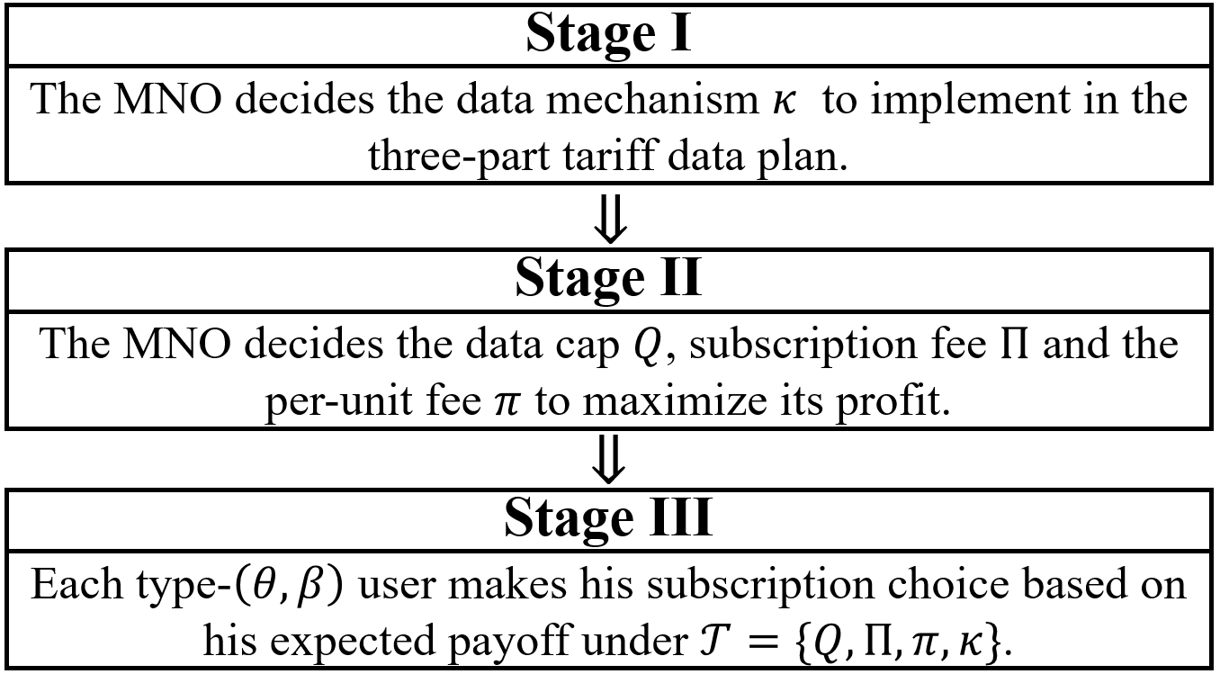
We formulate the economic interactions between the MNO and the mobile users as a three-stage Stackelberg game, as shown in Fig. 1. The MNO is the Stackelberg leader: it first decides the data mechanism to be implemented within its three-part tariff data plan in Stage I, then decides the data cap, the subscription fee, and the per-unit fee in Stage II.33 3 In practice, an MNO adopts a data mechanism (i.e., rollover, credit, or the traditional one) for a relatively long time period (e.g., three or five years), while has the flexibility of updating data mechanism parameters (i.e., the data cap, monthly subscription fee, and the per-unit fee) more often (e.g., on a yearly basis). The three-stage formulation captures the MNO’s different decisions at different time scales. Finally, the users make their subscription decisions to maximize their payoffs in Stage III.
Next we first present a unifying framework of different mobile data plans, then introduce the model in more details from the perspectives of users and the MNO, respectively.
III-A Mobile Data Plans
The three-part tariff data plan with time flexibility can be characterized by the tuple , where the subscriber pays a fixed lump-sum subscription fee for the data usage up to the cap , beyond which the subscriber pays an overage fee for each unit of additional data consumption. Here represents different data mechanisms that gives the subscriber different degrees of time flexibility on their data consumption over time.
Next we first introduce the four data mechanisms, then demonstrate that the pure usage-based data plan and the flat-rate data plan are special cases of the tuple .
III-A1 Four Data Mechanisms
We consider four data mechanisms indexed by . The key differences among the different data mechanisms are the special data and the consumption priority. To be more specific, the special data could be the rollover data inherited from the previous month or the credit data that can be borrowed from the next month, both of which can enlarge a subscriber’s effective data cap (within which no overage fee involved) in the current month. Moreover, the consumption priority of the special data and the current monthly data cap further affects how much the effective data cap can be enlarged.
We summarize the key differences of the four data mechanisms in Table I. Here we use to denote a user’s data surplus () or data deficit () at the beginning of a month, and use to denote the corresponding effective data cap. More specifically,
- •
The case of denotes the traditional data mechanism without time flexibility. The subscriber has no data surplus or deficit, and the effective cap of each month is ;
- •
The case of denotes the rollover data mechanism offered by AT&T. The rollover data from the previous month is consumed after the current monthly data cap and expires at the end of the current month. Thus the effective cap of the current month is ;
- •
The case of denotes the rollover data mechanism offered by China Mobile. The rollover data from the previous month is consumed prior to the current monthly data cap and expires at the end of the current month. Thus the effective cap of the current month is ;
- •
The case of denotes the credit data mechanism proposed in this paper. The credit data is from the next month’s data cap ,44 4 Since users can only borrow data from the next one month’s data cap, is the maximal amount that can be borrowed. which is consumed after the current monthly data cap (with a data deficit from the previous month). Thus the effective cap of the current month is ;
As mentioned above, the time flexibility can enlarge the subscriber’s effective data cap. According to Table I, the effective data cap of the traditional data mechanism (i.e., ) is always ; while the potential maximal value of the effective data cap is for the rollover and credit data mechanisms (i.e., ). The larger the effective data cap is, the less overage usage is incurred, which will further change the users’ subscription decisions.
Table II provides a numerical example with five months’ data consumptions and the corresponding payments under the four data mechanisms. Among the four schemes, the last two schemes (i.e., ) lead to the same least total payment of , and the first scheme (i.e., ) leads to the maximum total payment of . Is this a coincidence? We will further discuss it in Section IV.
III-A2 Special Cases of Three-Part Tariff
Next we illustrate that the pure usage-based data plan and the flat-rate data plan are two special cases of the tuple , .
Under the pure usage-based data plan, the subscriber has a zero monthly data cap and only needs to pay a usage-based fee for each unit of data consumption. Therefore, we can denote the pure usage-based data plan as , where represents that the data mechanism index has no impact under the pure usage-based data plan (as there is no data cap).
Under the flat-rate data plan, the subscriber pays a fixed monthly subscription fee for unlimited data usage without any additional overage fee, thus the per-unit fee has no impact. Strictly speaking, the data cap of the flat-rate data plan is infinity. However, in this paper we model the user’s data demand as a random variable (to be defined in Section III-B), where is the maximal data demand. Therefore, in practice it is enough to set the data cap to be no less than to achieve the effect of a flat-rate plan. Accordingly, we denote the flat-rate data plan as , where , and represents that the per-unit fee and the data mechanism have no impact.
Our later analysis on the MNO’s optimal data plan is based on the general tuple . Meanwhile, we will characterize the conditions under which the MNO’s optimal three-part tariff with time flexibility would degenerate into the pure usage-based data plan or the flat-rate data plan .
III-B User Model
Next we introduce a user’s three characterizations: the data demand , the data valuation , and the network substitutability . Based on these, we derive a user’s expected payoff.
First, we model the user’s monthly data demand as a discrete random variable with a probability mass function , a mean value of , and a finite integer support . Here the data demand is measured in the minimum data unit (e.g, 1KB or 1MB according to the MNO’s billing practice).
Second, we follow [7] by denoting as a user’s utility from consuming one unit of data, i.e., the user’s data valuation. According to our market survey conducted in mainland China, falls into the range between 10 RMB/GB and 60 RMB/GB with a large probability. We will further discuss it in Section VI-A.
Third, we further explore a user’s behavior change when he reaches the effective data cap , since further data consumption leads to an additional payment. Although the user will still continue to consume data in this case, he will rely more heavily on other alternative networks (such as Wi-Fi). As in [14], we use the network substitutability to denote the fraction of overage usage shrink. A larger value represents more overage usage cut (thus a better network substitutability).
A user’s mobility pattern can significantly influence the availability of alternative networks. Hence, different users usually have heterogeneous network substitutabilities. For example, a businessman who is always on the road may have a poor network substitutability (hence has a small value of ); while a student can take the advantage of the school Wi-Fi network (hence has a large value of ). According to our market survey, falls into the range between 0.7 and 1 with a large probability. We will further discuss it in Section VI-A.
| Month | Jan. | Feb. | Mar. | Apr. | May | Total | |
| Data Consumption | 2GB | 2GB | 4GB | 4GB | 1GB | 13GB | |
| Payment | 50 | 50 | 65 | 65 | 50 | ||
| 0 | 1GB | 1GB | 0 | 0 | |||
| Payment | 50 | 50 | 50 | 65 | 50 | ||
| 0 | 1GB | 2GB | 1GB | 0 | |||
| Payment | 50 | 50 | 50 | 50 | 50 | ||
| 0 | 0 | 0 | -1GB | -2GB | |||
| Payment | 50 | 50 | 50 | 50 | 50 | ||
- •
Here the data cap is 3GB, the subscription fee is 50, the overage fee is 15GB, and denotes the data surplus or deficit of each month.
Without loss of generality, we normalize the total user population size to one in the rest of the paper. We assume that users are homogeneous in the data demand distribution , 55 5 According to the statistical analysis in [20],[21], users’ monthly demand can be estimated by a log-normal distribution. For analysis tractability, we consider a homogeneous demand distribution. In the future, we will consider the heterogeneous case and collect users’ data usage records to estimate the demand distributions as in [11, 15]. and investigate the heterogeneity in the data valuation and network substitutability . Therefore, we model each user by the two-dimensional characteristics , and define the whole user market as with probability density functions and , since our market survey shows that and are independent with the Pearson correlation coefficient less than . Furthermore, we denote as the subscriber set, i.e., the type- user subscribes to the MNO if and only if .
A subscriber’s payoff is the difference between his utility and total payment. More specifically, for a type- subscriber with units of data demand and an effective data cap , his actual data usage is , where . Moreover, we use to represent the MNO’s average quality of service (QoS).66 6 In practice, an MNO’s wireless data service depends on the network congestion, which has been studied before (e.g., [7, 2]). In this work, instead of modeling the detailed congestion-aware control, we are more interested in the long-term average quality of the MNO’s wireless data service. Mathematically, is a utility multiplicative coefficient, thus the subscriber’s utility is . In addition, the subscriber’s total payment consists of the subscription fee and the overage payment . Therefore, the payoff of a type- subscriber with units of data demand and an effective cap is given by
| (1) | ||||
where the data demand and the data surplus (or deficit) are two random variables that change in each month. After taking the expectation over and , we obtain a type- subscriber’s expected monthly payoff as
| (2) | ||||
Here is the type- subscriber’s expected monthly overage data consumption under the data mechanism , defined as follows:
| (3) | ||||
where the summation range of is from to the maximal demand , while the range of depends on the data mechanism , which is given in (14), (17), and (20). The represents the probability mass function of under the data mechanism . Moreover, is the key difference among the four data mechanisms, since the data mechanism affects a subscriber’s payoff through in (2). In Section IV, we will further explain how to compute and in detail.
Furthermore, the expected total payoff of the whole market under is the integration over all the subscribers in , as follows:
| (4) |
So far, we have introduced users’ characteristics and derived their payoffs. Next we move on to model the profit-maximizing MNO.
III-C MNO Model
In the following we formulate the MNO’s revenue, cost, and profit, respectively.
III-C1 MNO’s Revenue
The MNO’s revenue obtained from a subscriber consists of the subscription fee and the possibly overage fee. Therefore, the MNO’s revenue from a type- subscriber with units of data demand and an effective cap is
| (5) |
Since and are two random variables that change in each month, we take the expectation and obtain the MNO’s expected monthly revenue from a type- subscriber as follows:
| (6) | ||||
where is the type- subscriber’s expected overage usage. Again we will provide more details on in Section IV. Moreover, the MNO’s expected total revenue from the entire market under is
| (7) |
III-C2 MNO’s Cost
In reality, the MNO’s cost is quite a complicated function that is related to many factors [2]. In this paper, we consider two kinds of costs experienced by the MNO, i.e., the capacity cost and the operational cost.
The MNO’s capacity cost mainly arises from its capital expenditure (CapEx), the investment on its network capacity. In reality, the data cap helps the MNO manage the network congestion and ration the scarce network capacity [22], and most MNOs imposed the data cap to alleviate the network congestion [23]. Therefore, once the MNO decides a data cap to be offered in the market, it should make sure a corresponding network capacity is in place to support the traffic. Motivated by this phenomenon, we model the MNO’s capacity cost as an increasing function on the data cap . Intuitively, a larger data cap corresponds to a more severe network congestion, which requires more investment on the network capacity in advance. The MNO’s capacity investment affects the network congestion, which will change its QoS and eventually affect the user utility of consuming data. Here we will not incorporate the congestion-aware formulation in this work, but refer interested readers to the related studies in [7, 2].
Furthermore, the MNO’s operational expense (OpEx) mainly arises from the system management. After the MNO decides the mobile data plan to implement in the market, the subscribers’ total data consumption will affect the MNO’s operational expense. Specifically, the expected total data consumption from the whole market is
| (8) |
For analysis tractability, we follow [24] by considering a linear operational cost, and denote as the marginal operational cost from unit data consumption.77 7 Such a linear-form cost has been widely used to model an operator’s operational cost (e.g., [24, 25]). Accordingly, the MNO’s operational cost is .
Putting the capacity cost and the operational cost together, we compute the MNO’s expected total cost as follows:
| (9) |
III-C3 MNO’s Profit
The MNO’s profit is the difference between its revenue and cost. Hence the MNO’s expected total profit under is
| (10) |
So far we have introduced the four data mechanisms, users’ payoffs, and MNO’s profit. In the following, we first compare the degrees of time flexibility offered by the four data mechanisms in Section IV, then study the three-stage game in Section V.


IV Data Mechanisms and Time Flexibility
Recall that the numerical example in Table II shows that the total payments for are the same and the least, while the payment for is the most. In this section we will demonstrate that it is not a coincidence, but a general conclusion reflecting the data mechanisms’ degrees of time flexibility.
In the following, we introduce how to compute in Section IV-A, then answer Question 2 (i.e., which data mechanism is the most time-flexible) in Section IV-B.
IV-A Data Mechanisms
As mentioned in Section III-B, the key difference among the four data mechanisms is the distribution of the subscriber’s data surplus or deficit , which further determines according to (3). Particularly, for , the data surplus or deficit is always zero, i.e., , since it does not offer subscribers any special data. However, for , we need to consider the data demand dynamic between successive months.
We illustrate the transition of users’ data surplus or deficit between two successive months in Fig. 2. Specifically, the horizontal axis corresponds to users’ random data demand , and the vertical axis represents users’ data surplus or deficit for the next month (given his data surplus or deficit in the current month and the data demand ). The differences among the three red curves in Fig. 2 indicate the differences among the three data mechanisms .
In the following, we analyze the distribution and compute under the four data mechanisms.
IV-A1 Traditional Data Mechanism
For a subscriber, there is no special data to use, i.e., and . Thus we only need to take the expectation over the data demand . Thus is
| (11) |
IV-A2 Rollover Data Mechanism
For a subscriber, the special data is the rollover data from the previous month, which is consumed after the current monthly data cap. Therefore, the effective data cap consists of the monthly data cap and the rollover data surplus , i.e., . Fig. 2(a) plots the rollover data to the next month, denoted by , versus the subscriber’s data demand in the current month. Thus we know
| (12) |
Note that the rollover data to the next month only depends on the subscriber’s monthly data cap and the data demand , and is independent of the data surplus from the previous month. Therefore, the probability mass function is
| (13) |
Then we need to take the expectation over the data demand and the rollover data surplus to compute the expected overage usage , as follows:
| (14) |
IV-A3 Rollover Data Mechanism
For a subscriber, the special data is the rollover data from the previous month, which is consumed prior to the current monthly data cap. Therefore, the effective data cap is the same as that for , i.e., . However, the rollover data is consumed prior to the monthly cap. As showed in Fig. 2(b), we know
| (15) |
It is notable that the rollover data to the next month depends on the monthly data cap , data demand , and the rollover data surplus from the previous month, resulting in a Markov property on the rollover data surplus . The one-step transition probability of the rollover data surplus is given by
| (16) |
Then we can derive the stationary distribution of the rollover data surplus , denoted by , according to the above transition probability [26]. Thus is given by
| (17) |
IV-A4 Credit Data Mechanism
For a subscriber, the special data is the credit data borrowed from the next month, which is used after the current monthly data cap. Therefore, the effective data cap of a subscriber with a data deficit consists of the remaining current monthly data cap (with a deficit ) and the maximum credit data that he can borrow from the next month (which is ), i.e., . According to Fig. 2(c), the data deficit in the next month, denoted by , is given by
| (18) |
Similar to the case when , we note that the data deficit in the next month depends on the monthly data cap , the data demand , and the data deficit in the current month, which indicates a Markov property on the data deficit for . The corresponding one-step transition probability of the data deficit is
| (19) |
Similarly we can derive the stationary distribution of the data deficit and compute as follows
| (20) |
Now that we have demonstrated how to compute under the four data mechanisms, next we will compare the degree of time flexibility based on .
IV-B Time Flexibility
In the following we compare the degrees of time flexibility among the four data mechanisms and answer Question 2.
Definition 1 (Time Flexibility)
Consider two data mechanisms . The data mechanism has a better time flexibility than the data mechanism , denoted by , if and only if for an arbitrary data demand distribution , we have for all .
Definition 1 uses the type- subscriber’s expected overage data consumption to indicate the time flexibility of the data mechanism . Intuitively, the better time flexibility the data mechanism offers, the less overage usage is incurred by its subscribers under the same data cap for an arbitrary data demand distribution . Note that we require in the definition, this is because that the three-part tariff with time flexibility degenerates into the pure usage-based data plan if or the flat-rate data plan if . In these two extreme cases, any data mechanism has no impact.
Lemma 1 summarizes the time flexibility of the four data mechanisms. The proof is given in Appendix A.
Lemma 1
For an arbitrary data demand distribution , we have for all . Therefore, the four data mechanisms’ degrees of time flexibility satisfy .
Lemma 1 provides the answer to Question 2 that we mentioned in Section 1. The rollover data mechanism offered by China Mobile (i.e., ) and our proposed credit data mechanism (i.e., ) are both the most time-flexible. The traditional data mechanism (i.e., ) is the least time-flexible.
The reason why is twofolds. First, the two data mechanisms can expand the effective data cap with the same intensity, i.e., for . Second, the consumption priorities of the two data mechanisms specify that subscribers should first consume the earlier data, i.e., the rollover data prior to the current monthly data cap for , and the current monthly data cap prior to the credit data for .
The reason why is because of the irregular consumption priority for . Recall that the rollover data mechanism offered by AT&T (i.e., ) requires that the current monthly data cap is consumed prior to the rollover data from the previous month, which means the later data (i.e., current monthly data cap) would be consumed prior to the earlier data (i.e., rollover data from the previous month). Such an irregular consumption priority prevents subscribers from fully utilizing their data quota in the long run, hence reduces the degree of time flexibility. Nevertheless, it is still time flexible than the traditional data mechanism, i.e., .
So far we have compared the degree of time flexibility among the four data mechanisms. Next in Section V, we analyze the three-stage game.


V Backward Induction of the Three-stage Stackelberg Game
In this section, we study the Subgame Perfect Equilibrium (SPE, or simply referred to as equilibrium in this paper) of the three-stage Stackelberg game by backward induction.
V-A User’s Subscription in Stage III
In Stage III, each user makes his subscription choice given the data plan offered by the MNO.
The type- user has two choices. If he does not subscribe, his payoff will be zero.88 8 Here we normalize the non-subscription payoff to be zero. If the user has other options, for example, relying purely on Wi-Fi networks, the non-subscription payoff can be positive. Our analysis will still go through in that case with a simple constant shift. Hence the user will subscribe to the MNO if and only if brings him a non-negative expected monthly payoff, i.e., . Theorem 1 presents the MNO’s market share under the data plan . The proof is given in Appendix B.
Theorem 1 (Market Share)
The MNO’s market share under data plan is
| (21) |
where is referred to as the threshold valuation under and , which is given by
| (22) |
Based on Theorem 1, we further summarize the impacts of users’ characteristics and on their subscription decisions in Corollary 1 and Corollary 2, respectively.
Corollary 1
[Impact of Data Valuation] Given the network substitutability , it is more likely for a user to subscribe to the MNO as his data valuation increases.
Corollary 1 indicates that higher valuation users are more likely to subscribe to the MNO. However, Corollary 2 shows that the impact of network substitutability is more complicated.
Corollary 2
[Impact of Network Substitutability] Given the data valuation , there are three possibilities for the impact of network substitutability :
- •
Case 1 (): As the network substitutability improves, users are more likely to subscribe to the MNO.
- •
Case 2 (): As the network substitutability improves, users are less likely to subscribe to the MNO.
- •
Case 3 (): The network substitutability does not affect the subscription decision.
In Corollary 2, represents the total data consumption of a type- subscriber. This type of subscriber has so good a network substitutability that he stops using mobile data after his effective data cap is used up. Thus he only needs to pay the subscription fee in each month. Accordingly, represents the average payment per unit data that he uses in each month.
Therefore, Case 1 in Corollary 2 represents that the per-unit fee is more expensive compared with the subscription fee in terms of the average rate of a type- subscriber; Case 2 is the opposite of Case 1; Case 3 represents that the per-unit fee , and the subscription fee are comparable for type- subscribers.
Now we illustrate Corollary 2 in Fig. 3, where the two axises correspond to the user’s network substitutability and data valuation , respectively. The gray region denotes the subscriber set . The red arrow represents the direction where the network substitutability increases.
- •
Fig. 3(a): If the per-unit fee is more expensive than the average payment per unit data, i.e., , then the red arrow shows that the users with a better network substitutability are more likely to become subscribers, since they incur less overage usage and thus less additional payment.
- •
Fig. 3(b): If the average payment for unit data is more expensive than the per-unit fee , i.e., , then the red arrow shows that the users with a better network substitutability are less likely to become subscribers. This is because that they are not willing to pay for an expensive subscription fee, considering the cheap per-unit fee and their good alternative networks.
- •
Fig. 3(c): If the average payment for unit data and the per-unit fee are comparable and satisfy , then the network substitutability does not change users’ subscription decisions.
Later on we will show that under the MNO’s optimal pricing strategy, the market partition is Fig. 3(c).
Considering the subscription choice derived from Theorem 1, the MNO’s expected total profit is given by
| (23) | ||||
Next we will further analyze the MNO’s optimal data cap and pricing strategy in Stage II.
V-B Optimal Data Cap and Pricing Strategy in Stage II
In Stage II, the MNO determines the profit-maximizing data cap and the pricing strategy considering users’ subscription decisions from Stage III, given the data mechanism obtained in Stage I.
To make the presentation clear and reveal the key insights, we first present the MNO’s optimal pricing strategy given the data cap in Section V-B1, and then we introduce the MNO’s optimal data cap in Section V-B2. 99 9 The two-step presentation enables us to illustrate the key insights of the optimal pricing strategy for a particularly data cap. This is practically important, since the MNO usually adopt integral data caps for simplicity, e.g., 1GB, 2GB, and 3GB.
V-B1 Optimal Pricing Strategy
Given the data cap , the objective of MNO is to find the optimal subscription fee and per-unit fee that maximize its expected total profit, that is,
Problem 1 (Optimal Pricing Strategy)
| (24) |
Before analyzing Problem 1, we need to introduce the following assumption on the MNO’s QoS and marginal operational cost .
Assumption 1
The MNO’s QoS and marginal operational cost satisfy .
Assumption 1 is made to avoid a trivial case, where the MNO offers very poor wireless service such that it cannot benefit from the market. It is not a technical assumption that limits our analysis and results.
Now we characterize the MNO’s profit-maximizing subscription fee and per-unit fee in Theorem 2.
Theorem 2 (Optimal Pricing Strategy)
Given the data cap and the data mechanism , the MNO’s profit-maximizing subscription fee and per-unit fee satisfying the following conditions:
| (25) |
where and are the PDF and CDF of the data valuation . Furthermore, is unique for an arbitrary distribution with an increasing failure rate (IFR).1010 10 The increasing failure rate condition refers to increasing in . Many commonly used distributions, such as uniform distribution, gamma distribution, and normal distribution, satisfy this condition [27].
Based on Theorem 2, we summarize the impact of several parameters on the optimal per-unit fee and the optimal subscription fee in Proposition 1 and Proposition 2, respectively.
Proposition 1
The optimal per-unit fee increases in the MNO’s QoS and marginal operational cost . It dose not depend on the data mechanism or how large the data cap is.
Proposition 2
The optimal subscription fee is related to the data cap and the data mechanism in the following ways,
- •
increases in the data cap ,
- •
a better time flexibility corresponds to a higher subscription fee, i.e., for all .
Recall that Corollary 2 summarizes three possibilities for the impact of network substitutability . Moreover, the optimal subscription fee and the per-unit fee derived in Theorem 2 satisfy , which is the same as Case 3 discussed in Corollary 2. In this case, the threshold valuation (defined in (22)) is
| (26) |
which is independent of . This naturally leads to the following corollary on the market partition under the optimal pricing strategy.
Corollary 3
Under the optimal pricing strategy specified in Theorem 2, the network substitutability does not affect the subscription decision. That is, the type- user will subscribe to the MNO if and only if . The MNO obtains the market of
| (27) |
Corollary 3 reveals that the MNO tends to select its subscribers based only on their data valuations, while ignoring the network substitutability. The intuition behind such a pricing strategy is that the MNO can benefit from good network substitutability users’ subscription fee and poor network substitutability users’ overage fee. Therefore, there is no incentive for the MNO to exclude either type of users.
Furthermore, according to Corollary 3, the MNO’s market share under the optimal pricing strategy is fixed for any data cap and data mechanism . However, different data caps and data mechanisms bring the MNO different profit. Substitute and into the MNO’s expected total profit, then we obtain
| (28) | ||||
where is the mean of the network substitutability among the whole user market, which is given by
| (29) |
Next we move on to analyze the MNO’s optimal data cap, considering the pricing strategy derived in Theorem 2.
V-B2 Optimal Data Cap
The MNO needs to select a data cap to maximize its expected total profit . That is, the MNO needs to solve the following problem
Problem 2 (Optimal Data Cap)
| (30) |
where and are the MNO’s profit-maximizing subscription fee and per-unit fee obtained from Theorem 2, respectively.
Problem 2 is not difficult to solve, since it is a single variable problem and is convex if is convex. To illustrate the key insights of the optimal data cap, hereafter, we follow [8] by making the following assumption on the MNO’s capacity cost throughout the rest of the paper.
Assumption 2
The MNO’s capacity cost takes a linear form, i.e., where is the marginal capacity cost.
Before analyzing the MNO’s optimal data cap, recall that the differences among the four data mechanisms is entirely captured in , the expected overage data consumption. To facilitate our later analysis, we refer to as the marginal overage data consumption, which is the absolute value of the derivative of with respect to . Specifically, the marginal overage data consumption measures the overage data usage decrement for a unit data cap increment on the data cap under the data mechanism .
Now we characterize the MNO’s optimal data cap in Theorem 3. The proof of Theorem 3 is given in Appendix D.
Theorem 3 (Optimal Data Cap)
Given the data mechanism , the MNO’s optimal data cap satisfies
| (31) |
where is given by
| (32) |
Theorem 3 indicates that no matter which data mechanism that the MNO adopts, the MNO should always choose a data cap such that the corresponding marginal overage data consumption equals to . Therefore, we refer to as the target marginal overage data consumption that the MNO must achieve to maximize its profit. Note that the target marginal overage data consumption is related to the MNO’s QoS , marginal operational cost , and the marginal capacity cost . Therefore, we further summarize how the three parameters affect the optimal data cap in Proposition 3.
Proposition 3
The MNO’s optimal data cap increases in the QoS , meanwhile decreases in the MNO’s marginal operational cost and marginal capacity cost .
Now we have characterized the optimal data cap in Theorem 3, and revealed how the MNO’s QoS (i.e., ) and marginal costs (i.e., and ) affect it. Next we analyze the impact of the data mechanism on the optimal data cap, which is related to Question 4 mentioned in Section 1.
Intuitively, we would think that the MNO can set a smaller cap under a data mechanism with a better time flexibility (to reduce the capacity cost), since it is more time-flexible for subscribers. In the following, however, we will reveal a counter-intuitive insight, i.e., a better time flexibility does not necessarily correspond to a smaller data cap.
To fully reveal this counter-intuitive insight, we need to know the detail mathematical expression of according to (31) in Theorem 3. Even though we cannot analytically compute due to the complexity of the Markov transition matrix, we are able to characterize some properties of in Lemma 2. The proof is given in Appendix E.
Lemma 2
For an arbitrary data demand distribution , is decreasing and convex in . Moreover, , , , and for all .
To illustrate the counter-intuitive insight, let us consider two data mechanisms , where offers a better time flexibility, i.e., .
Based on Lemma 2 and Definition 1, we can plot and versus the data cap in Fig. 4(a), and the corresponding marginal overage data consumptions and in Fig. 4(b).1111 11 Note that in Fig. 4(b) there is only one crossing point for and when . Basically, Lemma 2 cannot imply the uniqueness of the crossing point for an arbitrary demand distribution . Nevertheless, it does not affect the counter-intuitive insight, i.e., a better time flexibility does not necessarily correspond to a smaller data cap.


According to Theorem 3, the optimal data cap must make the corresponding marginal overage data consumption equal to the target marginal overage data consumption, i.e., . In Fig. 4(b), we consider two different target marginal overage data consumptions and , which correspond to different values of , , and .
- •
To achieve a small target marginal overage data consumption , the corresponding optimal data caps satisfy , indicating that the data mechanism (with a better time flexibility) leads to a smaller data cap;
- •
To achieve a large target marginal overage data consumption , the corresponding optimal data caps satisfy , indicating that the data mechanism (with a better time flexibility) leads to a larger data cap.
Later we will further illustrate this counter-intuitive insight in Section VI-B.
So far we have fully characterized the optimal data cap together with the impact of the data mechanism as well as the MNO’s QoS and costs. Next we will move on to study the MNO’s optimal data mechanism in Stage I.


V-C Optimal Data Mechanism in Stage I
In Stage I, the MNO determines the optimal data mechanism to maximize its expected total profit, which answers Question 3 mentioned in Section 1.
Problem 3 (Optimal Data Mechanism)
| (33) |
Lemma 3 reveals that a better time flexibility can always bring the MNO a higher profit under the optimal pricing strategy specified in Theorem 2 and the optimal data cap specified in Theorem 3, which naturally leads to Theorem 4.
Lemma 3
Consider two data mechanism , and the data mechanism has a better time flexibility than , i.e., . Then the following is true
| (34) |
where the equality holds if and only if or .
Theorem 4 (Optimal Data Mechanism)
Among the four data mechanisms , the MNO’s optimal data mechanism is and .
Theorem 4 shows that the MNO should adopt the rollover mechanism offered by China Mobile or the credit mechanism proposed in this paper to maximize its profit.
Next, we examine the conditions of the system parameters under which the optimal three-part tariff data plan degenerates into the pure usage-based plan or the flat-rate plan, in which case the choice of data mechanism has no effect on the subscribers.
Corollary 4 (Pure Usage-Based Plan)
If the target marginal overage data consumption , then the MNO maximizes its expected total profit by offering the pure usage-based data plan .
The condition in Corollary 4 is satisfied when the MNO
- •
provides poor services, i.e., is small, or
- •
experiences a large cost, i.e., or is large.
The above insight is consistent with the reality. From the users’ perspective, they are not willing to pay for any cap if the MNO’s QoS is poor. From the MNO’s perspective, it is not beneficial for it to incentivize more data consumption through a large data cap, if it experiences a large cost from network investment or system management.
As we mentioned in Section 1, the flat-rate data plan appears earliest in the telecommunication market. However, most MNOs do not offer the flat-rate data plan anymore. The following corollary can provide an explanation for this phenomenon.
Corollary 5 (Flat-Rate Plan)
If the marginal capacity cost , then the MNO maximizes its expected total profit by offering the flat-rate data plan .
Obviously, the condition in Corollary 5 corresponds to an extreme case that does not approximate the current reality well [28], which explains why the flat-rate data plan has ended in the past.


VI Numerical Results
To examine the performance of different data mechanisms, we collected some real data from the telecommunication market in mainland China1212 12 The related data is obtained through a survey, and the questionnaire is available through https://www.wjx.cn/jq/16895923.aspx.. In Section VI-A, we analyze the distributions of the data valuation and the network substitutability. In Section VI-B, we simulate the optimal data plan and investigate the effect of the time flexibility on users’ payoffs and the MNO’s profit.
VI-A Empirical Results
To estimate the statistic information of users’ data valuation and network substitutability , we collected some mobile users’ behavioral data from the telecommunication market in mainland China. The PDFs of these two parameters and are shown by the green bars in Fig. 5(a) and Fig. 5(b), respectively. We observe that a large proportion of users’ data valuations falls into the range between RMB/GB to RMB/GB, and most people would like to shrink of their overage data demand. Moreover, we also find that the Pearson correlation coefficient between and is less than 0.05, which allows us to fit the two distributions independently.
Next we estimate the data valuation PDF by assuming a gamma distribution, which satisfies the increasing failure rate (IFR). The PDF of a gamma distribution in the shape-rate parametrization is
| (35) |
where is a complete gamma function. We choose the parameters and by minimizing the least-squares divergence between the estimated and empirical PDF. In Fig. 5(a), the black curve is the estimated PDF. Visually, it is qualitatively similar to the empirical PDF. To further investigate the goodness-of-fit statistically, we use the Kolmogorov-Smirnov test on the null hypothesis that the data valuation comes from the gamma distribution, at the significance level of (i.e., if the Kolmogorov-Smirnov test returns a -value less than 0.05, then we need to reject this hypothesis) [29]. The test shows a -value of , hence the hypothesis that the data valuation follows the gamma distribution is valid.
Next we estimate the network substitutability PDF by assuming a truncated normal distribution, since the network substitutability has a concrete upper bound and lower bound, i.e., . The PDF of a normal distribution truncated between is
| (36) |
where is the probability density function of the standard normal distribution, and is its cumulative distribution function. Similarly, we find the truncated normal distribution by minimizing the least-squares divergence between the estimated and empirical PDFs. The corresponding Kolmogorov-Smirnov test shows a -value of , hence the hypothesis of the truncated normal distribution is valid.
VI-B Performance Evaluation
Next we will use the fitted market distribution to investigate how the MNO’s QoS and marginal costs affect its optimal data plan, and examine the impact of time flexibility on the users’ payoff and the MNO’s profit.
We set the minimum data unit to 1MB. Following the data analysis results in [20],[21], we assume that users’ monthly data demand follows a truncated log-normal distribution with a mean on the interval , i.e., the mean value is GB and the maximal usage is GB. Fig. 6 shows the PMF and the expected monthly overage usage under the four data mechanisms, which indicates that for all . Since the degree of time flexibility under and is equivalent, in the following we will neglect and only plot the results for .


VI-B1 Optimal Data Plan
We investigate the impact of QoS , marginal operational cost , and the marginal capacity cost individually.
In Fig. 7, we use three sub-figures to plot the optimal data cap versus the MNO’s QoS , marginal operational cost , and the marginal capacity cost , respectively. In addition, the three curves in each sub-figure correspond to the three data mechanisms .
Overall, the optimal data cap increases (from zero) as the MNO becomes stronger, in terms of
Particularly, the pure usage-based data plan appears when the MNO’s QoS in Fig. 7(a), marginal operational cost RMB/GB in Fig. 7(b), or marginal capacity cost RMB/GB in Fig. 7(c). In addition, Fig. 7(c) shows that the flat-rate data plan appears when , since the corresponding data cap is the maximal data demand GB.
As we mentioned in Section V-B2, a better time flexibility does not necessarily correspond to a smaller data cap. By comparing the three curves in each sub-figure of Fig. 7, we find that a better time flexibility would lead to an even larger data cap if the MNO is weak in terms of
The intuitions behind the counter-intuitive result include
- •
When the MNO is weak, it chooses a small data cap, under which the main revenue comes from users’ overage payments. In this case, offering a better time flexibility can significantly reduce its revenue from users’ overage payments. Therefore, the MNO will increase the data cap and the subscription fee to compensate its revenue loss.
- •
When the MNO is strong, it chooses a large data cap, under which its main revenue comes from users’ subscription fee. In this case, offering a better time flexibility does not reduce its revenue too much, and the MNO will decrease the data cap to further reduce its cost.
Next we examine the impact of the time flexibility on the monthly subscription fee.
Fig. 8 plots the optimal subscription fee under different data mechanisms. By comparing the three curves in each sub-figure, we observe that a higher subscription fee is always associated with a data mechanism with better time flexibility, even though it may correspond to a smaller or larger data cap as shown in Fig. 7.
The above discussions together with Proposition 1 provide answers to Question 4 mentioned in Section 1: a better time flexibility corresponds to a smaller data cap if the MNO is strong or a larger data cap if the MNO is weak. Meanwhile, a better time flexibility always leads to a higher subscription fee . Finally, it does not affect the optimal per-unit fee .
VI-B2 Users’ Payoffs and MNO’s Profit
We investigate the performance of different data mechanisms in terms of all users’ payoffs and the MNO’s profit. Specifically, we set the traditional data mechanism as the benchmark, and plot the performance gain of other schemes comparing to the benchmark. The three sub-figures in Fig. 9 plot the performance gains versus the MNO’s QoS , marginal operational cost , and the marginal capacity cost , respectively. The two solid curves in each sub-figure correspond to the MNO’s profit gains for , the other two dash curves represent users’ payoff gains for .
Overall, Fig. 9 show that the users’ payoff gains (i.e., the dash curves) decrease as the MNO’s QoS increases as in Fig. 9(a) or the MNO’s marginal costs and decrease as in Fig. 9(b) and Fig. 9(c). In this process, however, the MNO’s profit gains (i.e., the solid curves) first increase then decrease in all three sub-figures.
From the two solid curves in each sub-figure of Fig. 9, we find that the MNO’s profit gains under and are both non-negative, thus the time flexibility can increase the profit of MNO compared with the benchmark . From the two dash curves in each sub-figure of Fig. 9, we find that the users’ payoffs gains under and are both non-negative, thus the time flexibility increases the users’ payoffs as well. Moreover, we also note that always outperforms in terms of both MNO’s profit gain and users’ payoffs gain, which indicates that a better time flexibility leads to a larger improvement.
Now we know that both the MNO and the users can benefit from the time flexibility, a natural question is who will benefit more? By comparing the two red curves with squares (or the two blue curves with triangles) in each sub-figure, we find that the MNO benefits more from the time flexibility than users if the MNO is strong, in terms of
Intuitively, a stronger MNO has a larger pricing power, thus the strong MNO can benefit more than users from adding time flexibility. However, a weaker MNO has to leave users more benefits to maintain its market, thus users benefit more than a weaker MNO from time flexibility.
Furthermore, we also investigate the impact of the variances of the demand distribution, which indicates that the performance gain of the MNO’s profit and users’ payoff will increase in the variance. Due to the space limit, please refer to Appendix F for more detailed discussions.
The above discussions answer Question 1 in Section 1. In a monopoly market, both the MNO and users can benefit from a better time flexibility. Moreover, the MNO benefits more if the MNO offers good services and experiences small costs. Otherwise, the users benefit more.
VII Conclusions and Future Works
In this paper, we study the MNO’s optimal three-part tariff plan with time flexibility. Specifically, we consider four data mechanisms, and formulate the MNO’s optimal data plan design problem as a three-stage Stackelberg Game. Through backward induction, we analytically characterize the users’ subscription choices in Stage III, the MNO’s optimal data cap and corresponding pricing strategy in Stage II, and the MNO’s optimal data mechanism in Stage I. Moreover, we conduct a market survey to estimate the distribution of users’ data valuation and the network substitutability. Then we evaluate the performance of different data mechanisms using the real data.
In the future work, we want to collect more empirical data to estimate the MNO’s cost and users’ data demand distributions, and validate the insights obtained based on the current linear costs model and homogeneous data demand distribution. Moreover, we will consider a more general competitive market, and analyze the impact of time flexibility on multiple MNOs’ competition.
References
- [1] Z. Wang, L. Gao, and J. Huang, “Pricing optimization of rollover data plan,” in 15th International Symposium on Modeling and Optimization in Mobile, Ad Hoc, and Wireless Networks (WiOpt), 2017.
- [2] S. Sen, C. Joe-Wong, S. Ha, and M. Chiang, “Smart data pricing: using economics to manage network congestion,” Communications of the ACM, vol. 58, no. 12, pp. 86–93, 2015.
- [3] . [Online]. Available: https://www.att.com
- [4] T-mobile. [Online]. Available: https://support.t-mobile.com
- [5] China mobile. [Online]. Available: http://www.10086.cn
- [6] Data bank. [Online]. Available: http://bank.wo.cn/pc/home.html
- [7] R. T. Ma, “Usage-based pricing and competition in congestible network service markets,” IEEE/ACM Transactions on Networking, vol. 24, no. 5, pp. 3084–3097, 2016.
- [8] W. Dai and S. Jordan, “The effect of data caps upon isp service tier design and users,” ACM Transactions on Internet Technology (TOIT), vol. 15, no. 2, p. 8, 2015.
- [9] X. Wang, R. T. Ma, and Y. Xu, “The role of data cap in optimal two-part network pricing,” IEEE/ACM Transactions on Networking, vol. 25, no. 6, pp. 3602–3615, 2017.
- [10] Z. Xiong, S. Feng, D. Niyato, P. Wang, and Y. Zhang, “Economic analysis of network effects on sponsored content: a hierarchical game theoretic approach,” in IEEE Global Communications Conference (GLOBECOM), 2017.
- [11] L. Zheng, C. Joe-Wong, M. Andrews, and M. Chiang, “Optimizing data plans: Usage dynamics in mobile data networks,” in IEEE International Conference on Computer Communications (INFOCOM), 2018.
- [12] L. Zheng and C. Joe-Wong, “Understanding rollover data,” in Smart Data Pricing Workshop, 2016.
- [13] Y. Wei, J. Yu, T. M. Lok, and L. Gao, “A novel mobile data plan design from the perspective of data period,” in IEEE International Conference on Communication Systems (ICCS), 2016.
- [14] S. Sen, C. Joe-Wong, and S. Ha, “The economics of shared data plans,” in Annual Workshop on Information Technologies and Systems, 2012.
- [15] L. Zheng, C. Joe-Wong, C. W. Tan, S. Ha, and M. Chiang, “Customized data plans for mobile users: Feasibility and benefits of data trading,” IEEE journal on selected areas in communications, vol. 35, no. 4, pp. 949–963, 2017.
- [16] J. Yu, M. H. Cheung, J. Huang, and H. V. Poor, “Mobile data trading: Behavioral economics analysis and algorithm design,” IEEE Journal on Selected Areas in Communications, vol. 35, no. 4, pp. 994–1005, 2017.
- [17] L. Duan, J. Huang, and B. Shou, “Pricing for local and global wi-fi markets,” IEEE Transactions on Mobile Computing, vol. 14, no. 5, pp. 1056–1070, 2015.
- [18] Q. Ma, Y.-F. Liu, and J. Huang, “Time and location aware mobile data pricing,” IEEE Transactions on Mobile Computing, vol. 15, no. 10, pp. 2599–2613, 2016.
- [19] Z. Wang, L. Gao, and J. Huang, “Pricing competition of rollover data plan,” 16th International Symposium on Modeling and Optimization in Mobile, Ad Hoc, and Wireless Networks (WiOpt), 2018.
- [20] A. Lambrecht, K. Seim, and B. Skiera, “Does uncertainty matter? consumer behavior under three-part tariffs,” Marketing Science, vol. 26, no. 5, pp. 698–710, 2007.
- [21] A. Nevo, J. L. Turner, and J. W. Williams, “Usage-based pricing and demand for residential broadband,” Econometrica, vol. 84, no. 2, pp. 411–443, 2016.
- [22] W. P. Rogerson and E. Charles, “The economics of data caps and free data services in mobile broadband,” CTIA report, 2016.
- [23] D. A. Lyons, “The impact of data caps and other forms of usage-based pricing for broadband access,” Mercatus Center Working Papers, 2012.
- [24] P. Nabipay, A. Odlyzko, and Z.-L. Zhang, “Flat versus metered rates, bundling, and “bandwidth hogs”,” in 6th Workshop on the Economics of Networks, Systems, and Computation, 2011.
- [25] L. Duan, J. Huang, and B. Shou, “Duopoly competition in dynamic spectrum leasing and pricing,” IEEE Transactions on Mobile Computing, vol. 11, no. 11, pp. 1706–1719, 2012.
- [26] R. F. Bass, Stochastic processes. Cambridge University Press, 2011.
- [27] X. Brusset, “Properties of distributions with increasing failure rate,” MPRA Paper 18299, University Library of Munich, 2009.
- [28] E. J. Oughton and Z. Frias, “The cost, coverage and rollout implications of 5G infrastructure in britain,” Telecommunications Policy, 2017.
- [29] F. J. Massey Jr, “The kolmogorov-smirnov test for goodness of fit,” Journal of the American statistical Association, vol. 46, no. 253, pp. 68–78, 1951.
![[Uncaptioned image]](1808.10569v3/wang-photo.jpg) |
Zhiyuan Wang received the B.S. degree from Southeast University, Nanjing, China, in 2016. He is currently working toward the Ph.D. degree with the Department of Information Engineering, The Chinese University of Hong Kong, Shatin, Hong Kong. His research interests include the field of network economics and game theory, with current emphasis on smart data pricing and fog computing. He is the recipient of the Hong Kong PhD Fellowship. |
![[Uncaptioned image]](1808.10569v3/gao-photo.jpg) |
Lin Gao (S’08-M’10-SM’16) received the PhD degree in electronic engineering from Shanghai Jiao Tong University in 2010 and worked as a postdoctoral research fellow with the Chinese University of Hong Kong from 2010 to 2015. He is an associate professor in the School of Electronic and Information Engineering, Harbin Institute of Technology, Shenzhen, China. He received the IEEE ComSoc Asia-Pacific Outstanding Young Researcher Award in 2016. His main research interests are in the area of network economics and games, with applications in wireless communications and networking. He has co-authored 3 books including the textbook Wireless Network Pricing by Morgan & Claypool (2013). He is the co-recipient of three Best (Student) Paper Awards from WiOpt 2013, 2014, 2015, and is a Best Paper Award Finalist from IEEE INFOCOM 2016. |
![[Uncaptioned image]](1808.10569v3/huang-photo.jpg) |
Jianwei Huang (F’16) is a Professor and Director of the Network Communications and Economics Lab (ncel.ie.cuhk.edu.hk), in the Department of Information Engineering at the Chinese University of Hong Kong. He received the Ph.D. degree from Northwestern University in 2005, and worked as a Postdoc Research Associate at Princeton University during 2005-2007. He is an IEEE Fellow, a Distinguished Lecturer of IEEE Communications Society, and a Clarivate Analytics Highly Cited Researcher in Computer Science. Jianwei Huang is the co-author of 9 Best Paper Awards, including IEEE Marconi Prize Paper Award in Wireless Communications in 2011. He has co-authored six books, including the textbook on ”Wireless Network Pricing.” He received the CUHK Young Researcher Award in 2014 and IEEE ComSoc Asia-Pacific Outstanding Young Researcher Award in 2009. He has served as an Associate Editor of IEEE Transactions on Mobile Computing, IEEE/ACM Transactions on Networking, IEEE Transactions on Network Science and Engineering, IEEE Transactions on Wireless Communications, IEEE Journal on Selected Areas in Communications - Cognitive Radio Series, and IEEE Transactions on Cognitive Communications and Networking. He has served as an Editor of Wiley Information and Communication Technology Series, Springer Encyclopedia of Wireless Networks, and Springer Handbook of Cognitive Radio. |
Appendix A Proof of Lemma 1
In order to prove Lemma 1, in the following three subsections, we prove , , and , respectively.
A-A Proof of
We prove by computing the weighted summations in two steps. Specifically, and are given by
| (37) | ||||
It is obvious that the following inequality is true
| (38) |
Now we compute the weighted summation over the weight for (38), and we obtain
| (39) |
which is equivalent to
| (40) |
Then we further compute the weighted summation over the weight for (40), and we obtain
| (41) |
which implies .
A-B Proof of
Second, we prove through transforming their mathematical expressions. Specifically, and are given by
| (42) | ||||
As mentioned in Section IV-A, for , the data deficit of the next month is
| (43) |
Here we further define and , thus
| (44) |
Now we substitute into (44), and get
| (45) |
Therefore, the transition matrix from to is
| (46) |
which is the same as the transition matrix of the data mechanism derived in (16). Thus they have the same stationary distribution, i.e., for any .
Now we substitute into (42), and obtain
| (47) |
A-C Proof of
Now we prove . Specifically, and are given by
| (48) |
| (49) |
The only difference between (48) and (48) lies in the stationary distribution and . Due to the complexity of the Markov chain specified in (16), we are not able to compute the closed-form expression for and . Nevertheless, we will prove by showing that for an arbitrary realized data demand sequence, the overage data consumption under is larger than that under .
We consider months, i.e., . We denote as the realized data demand sequence, where denotes the realized data demand in month . Moreover, we denote and as the subscriber’s data surplus under the data mechanism and at the beginning of month .
Therefore, given the realized data usage sequence , the subscriber’s overage data consumption in month is
| (50) |
Next we first introduce Lemma 4.
Lemma 4
For any realized data demand sequence , we have and for any .
First, if , then , thus we know . Hence, Lemma 4 is true when .
Second, we assume that Lemma 4 is true for , and consider the case of .
We first show that . According to we consumption priority, we know that is
| (51) |
and is
| (52) |
Based on (51) and (52), we know that
- •
If , then for any .
- •
If , then we have the following relation between and ,
(53)
Therefore, we find that . Next we show that . According to the following formulation
| (54) |
we know that
- •
If , then we have for any realized data demand sequence .
- •
If , then we have the following relation between and ,
(55)
Appendix B Proof of Theorem 1
A type- subscriber’s expected monthly payoff is
| (57) |
by solving , we obtain
| (58) |
thus the market share of the MNO under the data plan is
| (59) |
Appendix C Proof of Theorem 2
We prove Theorem 2 by deriving the MNO’s profit-maximizing subscription fee and per-unit fee. Recall that the profit of the MNO is given by
| (60) | ||||
Since we consider a fixed in Theorem 2, then is a constant, and we denote it as . Accordingly, we obtain
| (61) | ||||
where is given by
| (62) |
Therefore, we can write as
| (63) |
Note that, under the assumption that distribution satisfies the increasing failure rate (i.e., increases in ), we have the following inequality
| (65) |
where is uniquely determined by
| (66) |
since decreases in and increases in .
Appendix D Proof of Theorem 3
We prove Theorem 3 by deriving the MNO’s profit-maximizing data cap. Under the optimal pricing strategy, the MNO’s expected total profit is given by
| (70) | ||||
which is concave on the data cap , since is convex on and is linear on . We take the derivative of (70) with respect to the data cap , and obtain the following optimality condition
| (71) |
which is equivalent to
| (72) |
Recall that the optimal per-unit fee satisfies
| (73) |
which means that
| (74) |
Appendix E Proof of Lemma 2
We prove Lemma 2 by computing , , , and , and showing the convexity of on . Recall that the mathematic expression of is
| (77) | ||||
E-A Compute and
When substituting and into , respectively, we obtain
| (78) | ||||
E-B Compute , and
We compute the derivative of with respect to as follows:
| (79) |
When substituting into (79), we obtain as following
| (80) |
Now we can compute by substituting into (80), as follows
| (81) |
Similarly, we are able to show that for any .
Furthermore, when substituting into (79), we obtain as follows
| (82) |
Now we can compute by substituting into (82), as follows
| (83) |
Similarly, we are able to show that for any .
E-C Convexity
According to (77), is the nonnegative weighted summation over . Specifically, is given by
| (84) |
which indicates that is always convex in for any . Considering the nonnegative weighted summation is a convexity-preserving operation, thus is convex in .
Appendix F Variance of Demand Distribution
We investigate the impact of the demand distribution variance by considering two different values. Specifically, we consider two log-normal distributions, which have the same mean value of 1GB but different variances (i.e., ). In the following, we first show the distributions and the expected overage payments, then compare the performance gains under the two values of variances.
Fig. 10 shows the demand distributions and the corresponding expected overage payment. The horizontal axis in each sub-figure corresponds to the MNO’s QoS. By comparing Fig. 10(a) and Fig. 10(b), we note that given the same data mechanism (e.g., with two red curves in the two sub-figures), a larger demand variance leads to higher expected overage payments. The impact of time-flexible data mechanism on reducing overage payment is stronger under a larger variance, since the differences among the three curves with markers in Fig. 10(a) is larger than that in Fig. 10(b).
Fig. 11 plots the performance gain of the time-flexible data mechanisms (compare with the traditional data mechanism) under the two values of variance. We note that a larger variance leads to a higher gain for both MNO’s profit gain and users’ payoff gain.
Based on the above discussions, we find that the time-flexible data mechanism plays a significant role, especially when the users’ demand variance is relatively large.


