跳到论文正文
W Papers独立论文阅读器 arXiv:1808.10532 论文正文 计算阅读时间 · 0%
引用这篇论文根据当前论文元数据生成,正式投稿前建议核对。


License: arXiv.org perpetual non-exclusive license
arXiv:1808.10532v2 [stat.ME] 03 Dec 2018

Uniform Inference in High-Dimensional Gaussian Graphical Models??

Sven Klaassen     Jannis Kück     Martin Spindler     Victor Chernozhukov

Graphical models have become a very popular tool for representing dependencies within a large set of variables and are key for representing causal structures. We provide results for uniform inference on high-dimensional graphical models with the number of target parameters dd being possible much larger than sample size. This is in particular important when certain features or structures of a causal model should be recovered. Our results highlight how in high-dimensional settings graphical models can be estimated and recovered with modern machine learning methods in complex data sets. To construct simultaneous confidence regions on many target parameters, sufficiently fast estimation rates of the nuisance functions are crucial. In this context, we establish uniform estimation rates and sparsity guarantees of the square-root estimator in a random design under approximate sparsity conditions that might be of independent interest for related problems in high-dimensions. We also demonstrate in a comprehensive simulation study that our procedure has good small sample properties.

, ,
 and

1 Introduction

We provide methodology and theory for uniform inference on high-dimensional graphical models with the number of target parameters being possible much larger than sample size. We demonstrate uniform asymptotic normality of the proposed estimator over dd-dimensional rectangles and construct simultaneous confidence bands on all of the dd target parameters. The proposed method can be applied to test simultaneously the presence of a large set of edges in the graphical model

X=(X1,…,Xp)T∼𝒩⁡(μX,ΣX).X=(X_{1},\dots,X_{p})^{T}\sim\mathcal{N}(\mu_{X},\Sigma_{X}).

Assuming that the covariance matrix ΣX\Sigma_{X} is nonsingular, the conditional independence structure of the distribution can be conveniently represented by a graph G=(V,E)G=(V,E), where V={1,…,p}V=\{1,\dots,p\} is the set of nodes and EE the set of edges in V×VV\times V. Every pair of variables not contained in the edge set is conditionally independent given all remaining variables. If the vector XX is normally distributed, every edge corresponds to a non-zero entry in the inverse covariance matrix (Lauritzen (1996)) [11].

In the last decade, significant progress has been made on estimation of a large precision matrix in order to analyze the dependence structure of a high-dimensional normal distributed random variable. There are mainly two common approaches to estimate the entries of a precision matrix. The first approach is a penalized likelihood estimation approach with a lasso-type penalty on entries of the precision matrix, typically referred to as the graphical lasso. This approach has been studied in several papers, see e.g Lam and Fan (2009) [10], Rothman et al. (2008) [15], Ravikumar et al. (2011) [13] and Yuan and Lin (2007) [20]. The second approach, first introduced by Meinshausen and Bühlmann (2006) [12], is neighborhood based. It estimates the conditional independence restrictions separately for each node in the graph and is hence equivalent to variable selection for Gaussian linear models. The idea of estimating the precision matrix column by column by running a regression for each variable against the rest of variables was further studied in Yuan (2010) [19], Cai, Liu and Zhou (2011) [5] and Sun and Zhang (2013) [16].

In this paper, we do not aim to estimate the whole precision matrix but we focus on quantifying the uncertainty of recovering its support by providing a significance test for a set of potential edges. In recent years, statistical inference for the precision matrix in high-dimensional settings has been studied, e.g in Janková and van de Geer (2016) [9] and Ren et al. (2015) [14]. Both approaches lead to an estimate that is elementwise asymptotically normal and enables testing for low-dimensional parameters of the precision matrix using standard procedures such as Bonferroni-Holm correction.
In contrast to these existing results, our method explicitly allows for testing a joint hypothesis without correction for multiple testing and conducting inference for a growing number of parameters using high dimensional central limit results. In particular, our results rely on approximate sparsity instead of row sparsity which restricts the number of non-zero entries of each row of the precision matrix to be at most s≪ns\ll n that is in many applications a questionable assumption. In order to provide theoretical results, fitting the problem of support discovery in Gaussian graphical models into a general Z-estimation setting with a high-dimensional nuisance function is key. Inference on a (multivariate) target parameter in general Z-estimation problems in high dimensions is covered in Belloni et al. (2014) [3], Belloni et al. (2018) [2] and Chernozhukov et al. (2017) [6]. To conduct inference on a high-dimensional target parameter, uniform estimation rates and sparsity guarantees of the nuisance function are crucial. In this context, we formally apply recent results from Belloni et al. (2018) [2] to ensure sufficient fast convergence rate of the lasso estimator under approximate sparsity conditions. Moreover, we provide auxiliary results for the square-lasso estimator establishing uniform estimation rates and sparsity guarantees in a random design under approximate sparsity conditions that might be of independent interest for related problems in high-dimensional linear models.

Plan of this Paper

The rest of this paper is organized as follows. In Section 2, we formally define the setting and introduce the notation that will be used fitting the problem of support discovery in Gaussian graphical models into a general Z-estimation problem with a high-dimensional nuisance function. In Section 3, we outline the estimation procedure of the high-dimensional target parameter and the conditions that are needed to achieve our main theorem presented in Section 4. Section 5 provides implementation details and shows how our estimation procedure can be modified by cross-fitting to improve small sample properties. Section 6 provides a simulation study on the proposed method. The supplementary material includes additional technical material. The proof of our main theorem is provided in Appendix A. The uniform nuisance function estimation is discussed in Appendix B. Appendix B.1 formally discusses conditions for the uniform convergence rates of the lasso estimator. Finally, Appendix B.2 provides auxiliary results for the square-lasso estimator.

2 Setting

Let

X=(X1,…,Xp)T∼𝒩⁡(μX,ΣX)X=(X_{1},\dots,X_{p})^{T}\sim\mathcal{N}(\mu_{X},\Sigma_{X})

be a pp-dimensional random variable. For all (j,k)∈E(j,k)\in E with j≠kj\neq k, assume that

Xj=∑l=1l≠jpβl(j)​Xl+ε(j)=β(j)​X−j+ε(j)X_{j}=\sum\limits_{\begin{subarray}{c}l=1\\ l\neq j\end{subarray}}^{p}\beta_{l}^{(j)}X_{l}+\varepsilon^{(j)}=\beta^{(j)}X_{-j}+\varepsilon^{(j)}

and

Xk=γ(j,k)​X−{j,k}+ν(j,k),X_{k}=\gamma^{(j,k)}X_{-\{j,k\}}+\nu^{(j,k)},

where 𝔼⁡[ε(j)|X−j]=0\mathbb{E}[\varepsilon^{(j)}|X_{-j}]=0 and 𝔼⁡[X−{j,k}​ν(j,k)]=0\mathbb{E}[X_{-\{j,k\}}\nu^{(j,k)}]=0. Define the column vector

Γ(j)=(−β1(j),…,−βj−1(j),1,−βj+1(j),…,−βp(j))T.\Gamma^{(j)}=\left(-\beta^{(j)}_{1},\dots,-\beta^{(j)}_{j-1},1,-\beta^{(j)}_{j+1},\dots,-\beta^{(j)}_{p}\right)^{T}.

One may show

Φ0=(Φ01,…,Φ0p)=(Γ(1)/V​a​r​(ε(1)),…,Γ(p)/V​a​r​(ε(p))),\displaystyle\Phi_{0}=\left(\Phi_{0}^{1},\dots,\Phi_{0}^{p}\right)=\left(\Gamma^{(1)}/Var(\varepsilon^{(1)}),\dots,\Gamma^{(p)}/Var(\varepsilon^{(p)})\right),

where Φ0j\Phi_{0}^{j} is the jj-th column of the precision matrix Φ0=ΣX−1\Phi_{0}=\Sigma_{X}^{-1} [9]. Hence

βk(j)=0⇔βj(k)=0⇔Xj⟂Xk|X−{j,k}\displaystyle\beta^{(j)}_{k}=0\Leftrightarrow\beta^{(k)}_{j}=0\Leftrightarrow X_{j}\perp X_{k}|X_{-\{j,k\}} (2.1)

for all j≠kj\neq k. Assume that we are interested in the following set of potential edges

ℳ:={m1,…,mdn}\mathcal{M}:=\{m_{1},\dots,m_{d_{n}}\}

where the number of edges dnd_{n} may increase with sample size nn. In the following the dependence on nn is omitted to simplify the notation. In order to test whether all variables XjX_{j} and XkX_{k} are conditionally independent with mr=(jr,kr)m_{r}=(j_{r},k_{r}) for a r∈{1,…,d}r\in\{1,\dots,d\}, we have to estimate our target parameter

θ0=(θm1,…,θmd)T:=(βk1(j1),…,βkd(jd))T.\theta_{0}=(\theta_{m_{1}},\dots,\theta_{m_{d}})^{T}:=(\beta^{(j_{1})}_{k_{1}},\dots,\beta^{(j_{d})}_{k_{d}})^{T}.

The setting above fits in the general Z-estimation problem of the form

𝔼⁡[ψmr​(X,θmr,ηmr)]=0\mathbb{E}\left[\psi_{m_{r}}\big(X,\theta_{m_{r}},\eta_{m_{r}}\big)\right]=0

for all r=1,…,dr=1,\dots,d with nuisance parameters

ηmr=(β−k(j),γ(j,k))\eta_{m_{r}}=\left(\beta^{(j)}_{-k},\gamma^{(j,k)}\right)

where β−k(j)≡β(mr)\beta^{(j)}_{-k}\equiv\beta^{(m_{r})} and γ(j,k)≡γ(mr)\gamma^{(j,k)}\equiv\gamma^{(m_{r})}. The score functions are defined by

ψmr​(X,θ,η):\displaystyle\psi_{m_{r}}(X,\theta,\eta): =(Xj−θ​Xk−η(1)​X−mr)​(Xk−η(2)​X−mr)\displaystyle=\Big(X_{j}-\theta X_{k}-\eta^{(1)}X_{-m_{r}}\Big)\Big(X_{k}-\eta^{(2)}X_{-m_{r}}\Big)

for mr=(jr,kr)≡(j,k)m_{r}=(j_{r},k_{r})\equiv(j,k), η=(η(1),η(2))\eta=(\eta^{(1)},\eta^{(2)}) and r=1,…,dr=1,\dots,d. Without loss of generality we assume j>kj>k for all tuples mr∈ℳm_{r}\in\mathcal{M}.

Comment 2.1.

The score function ψ\psi is linear, meaning

ψmr​(X,θ,η)=ψmra​(X,η(2))​θ+ψmrb​(X,η)\displaystyle\psi_{m_{r}}(X,\theta,\eta)=\psi_{m_{r}}^{a}(X,\eta^{(2)})\theta+\psi_{m_{r}}^{b}(X,\eta)

with

ψmra​(X,η(2))=−Xk​(Xk−η(2)​X−mr)\psi^{a}_{m_{r}}(X,\eta^{(2)})=-X_{k}\Big(X_{k}-\eta^{(2)}X_{-m_{r}}\Big)

and

ψmrb​(X,η)=(Xj−η(1)​X−mr)​(Xk−η(2)​X−mr)\psi^{b}_{m_{r}}(X,\eta)=\Big(X_{j}-\eta^{(1)}X_{-m_{r}}\Big)\Big(X_{k}-\eta^{(2)}X_{-m_{r}}\Big)

for mr=(j,k)m_{r}=(j,k) and r=1,…,dr=1,\dots,d.

It is well known that in partially linear regression models θ0\theta_{0} satisfies the moment condition

𝔼⁡[ψmr​(X,θmr,ηmr)]=0\displaystyle\mathbb{E}\left[\psi_{m_{r}}\big(X,\theta_{m_{r}},\eta_{m_{r}}\big)\right]=0 (2.2)

for all r=1,…,dr=1,\dots,d and also the Neyman orthogonality condition

∂t{𝔼⁡[ψmr​(X,θmr,ηmr+t​η~)]}|t=0\displaystyle\partial_{t}\left\{\mathbb{E}\left[\psi_{m_{r}}\big(X,\theta_{m_{r}},\eta_{m_{r}}+t\tilde{\eta}\big)\right]\right\}\big|_{t=0}

for all η~\tilde{\eta} in an appropriate set where ∂t\partial_{t} denotes the derivate with respect to tt. These properties are crucial for valid inference in high dimensional settings. We will show these properties explicitly in the proof of Theorem 1.

3 Estimation

Let X(i)X^{(i)}, i=1,…,ni=1,\dots,n be i.i.d. random vectors.
At first we estimate the nuisance parameter ηmr=(ηmr(1),ηmr(2))\eta_{m_{r}}=\big(\eta_{m_{r}}^{(1)},\eta_{m_{r}}^{(2)}\big) by running a lasso/ post-lasso/ square-root lasso regression of XjX_{j} on X−jX_{-j} to compute (θ~mr,η^mr(1))(\tilde{\theta}_{m_{r}},\hat{\eta}_{m_{r}}^{(1)}) and a lasso/ post-lasso/ square-root lasso regression of XkX_{k} on X−mrX_{-m_{r}} to compute η^mr(2)\hat{\eta}_{m_{r}}^{(2)} for each (j,k)=mr∈ℳ(j,k)=m_{r}\in\mathcal{M}. The estimator θ^0\hat{\theta}_{0} of the target parameter

θ0=(θm1,…,θmd)T\theta_{0}=(\theta_{m_{1}},\dots,\theta_{m_{d}})^{T}

is defined as the solution of

supr=1,…,d{|𝔼n​[ψmr​(X,θ^mr,η^mr)]|−infθ∈Θmr|𝔼n​[ψmr​(X,θ,η^mr)]|}≤ϵn,\displaystyle\sup\limits_{r=1,\dots,d}\left\{\left|\mathbb{E}_{n}\Big[\psi_{m_{r}}\big(X,\hat{\theta}_{m_{r}},\hat{\eta}_{m_{r}}\big)\Big]\right|-\inf_{\theta\in\Theta_{m_{r}}}\left|\mathbb{E}_{n}\Big[\psi_{m_{r}}\big(X,\theta,\hat{\eta}_{m_{r}}\big)\Big]\right|\right\}\leq\epsilon_{n}, (3.1)

where ϵn=o(δnn−1/2)\epsilon_{n}=o\left(\delta_{n}n^{-1/2}\right) is the numerical tolerance and (δn)n≥1(\delta_{n})_{n\geq 1} a sequence of positive constants converging to zero.

Assumptions A1-A4.
Let an:=max⁡(d,p,n,e)a_{n}:=\max(d,p,n,e) and CC a strictly positive constant independent of nn and rr. The following assumptions hold uniformly in n≥n0,P∈𝒫nn\geq n_{0},P\in\mathcal{P}_{n}:

  1. A1

    For all mr=(j,k)∈ℳm_{r}=(j,k)\in\mathcal{M} with j≠kj\neq k we have the following approximate sparse representations

    • (i)

      It holds

      Xj\displaystyle X_{j} =β(j)​X−j+ε(j)\displaystyle=\beta^{(j)}X_{-j}+\varepsilon^{(j)}
      =θmr​Xk+(β(1,mr)+β(2,mr))​X−mr+ε(mr)\displaystyle=\theta_{m_{r}}X_{k}+\left(\beta^{(1,m_{r})}+\beta^{(2,m_{r})}\right)X_{-m_{r}}+\varepsilon^{(m_{r})}

      with

      ‖β(1,mr)‖0≤s,maxr=1,…,d⁡‖β(2,mr)‖12≤C​s2​log⁡(an)n\|\beta^{(1,m_{r})}\|_{0}\leq s,\hskip 10.00002pt\max_{r=1,\dots,d}\|\beta^{(2,m_{r})}\|_{1}^{2}\leq C\sqrt{\frac{s^{2}\log(a_{n})}{n}}

      and

      maxr=1,…,d⁡𝔼⁡[(β(2,mr)​X−mr)2]≤C​s​log⁡(an)n.\max_{r=1,\dots,d}\mathbb{E}\left[\left(\beta^{(2,m_{r})}X_{-m_{r}}\right)^{2}\right]\leq C\frac{s\log(a_{n})}{n}.
    • (ii)

      It holds

      Xk\displaystyle X_{k} =γ(j,k)​X−{j,k}+ν(j,k)\displaystyle=\gamma^{(j,k)}X_{-\{j,k\}}+\nu^{(j,k)}
      =(γ(1,mr)+γ(1,mr))​X−mr+ν(mr)\displaystyle=\left(\gamma^{(1,m_{r})}+\gamma^{(1,m_{r})}\right)X_{-m_{r}}+\nu^{(m_{r})}

      with

      ‖γ(1,mr)‖0≤s,maxr=1,…,d⁡‖γ(2,mr)‖12≤C​s2​log⁡(an)n\|\gamma^{(1,m_{r})}\|_{0}\leq s,\hskip 10.00002pt\max_{r=1,\dots,d}\|\gamma^{(2,m_{r})}\|_{1}^{2}\leq C\sqrt{\frac{s^{2}\log(a_{n})}{n}}

      and

      maxr=1,…,d⁡𝔼⁡[(γ(2,mr)​X−mr)2]≤C​s​log⁡(an)n.\max_{r=1,\dots,d}\mathbb{E}\left[\left(\gamma^{(2,m_{r})}X_{-m_{r}}\right)^{2}\right]\leq C\frac{s\log(a_{n})}{n}.
  2. A2

    There exist positive numbers q~>0\tilde{q}>0 and κ<1\kappa<1 such that the following growth conditions are fulfilled:

    n1q~​s2​log4⁡(an)n=o⁡(1)​,log⁡(d)=o⁡(n19∧nκq~).\displaystyle n^{\frac{1}{\tilde{q}}}\frac{s^{2}\log^{4}(a_{n})}{n}=o(1)\text{,}\hskip 10.00002pt\log(d)=o\left(n^{\frac{1}{9}}\wedge n^{\frac{\kappa}{\tilde{q}}}\right).
  3. A3

    For all mr=(j,k)∈ℳm_{r}=(j,k)\in\mathcal{M} it holds

    ‖β(mr)‖2+‖γ(mr)‖2≤C\|\beta^{(m_{r})}\|_{2}+\|\gamma^{(m_{r})}\|_{2}\leq C

    and

    supr=1,…,dsupθ∈Θmr|θ|≤C.\sup\limits_{r=1,\dots,d}\sup\limits_{\theta\in\Theta_{m_{r}}}|\theta|\leq C.

    Additionally Θmr\Theta_{m_{r}} contains a ball of radius log(log(n))n−1/2log1/2(d)log(n)\log(\log(n))n^{-1/2}\log^{1/2}(d)\log(n) centered at θmr\theta_{m_{r}}.

  4. A4

    It holds

    inf‖ξ‖2=1𝔼⁡[(ξ​X)2]≥c​ and ​sup‖ξ‖2=1𝔼⁡[(ξ​X)2]≤C.\displaystyle\inf\limits_{\|\xi\|_{2}=1}\mathbb{E}\left[(\xi X)^{2}\right]\geq c\text{ and }\sup\limits_{\|\xi\|_{2}=1}\mathbb{E}\left[(\xi X)^{2}\right]\leq C.

The condition A1 is a standard approximate sparsity condition that is discussed in more detail in comment 3.1. The number of relevant variables sn≡ss_{n}\equiv s captured by the regression coefficient β(1,mr)\beta^{(1,m_{r})} respectively γ(1,mr)\gamma^{(1,m_{r})} can grow with the sample size. The coefficient β(2,mr)\beta^{(2,m_{r})} respectively γ(2,mr)\gamma^{(2,m_{r})} is the approximate sparse part of the true regression coefficient. This misspecification of a sparse model is controlled by condition A1. The growth condition A2 ensures that s2​log4⁡(an)/ns^{2}\log^{4}(a_{n})/n converges towards zero with at least polynomial speed. If this convergence is too slow (q~≥9\tilde{q}\geq 9) the condition on the growth rate of the number of tested edges become more restrictive. In general, both the number of parameters pp and the number of relevant variables ss can grow with the sample size in a balanced way. If ss is fixed, the number of potential parameters pp can grow at an exponential rate with the sample size. This means that the set of potential variables can be much larger than the sample size, only the number of relevant variables ss has to be smaller than the sample size. This situation is common for Lasso-based estimators. Condition A3 restricts the parameter spaces and ensures that the true coefficients are well behaved. The condition A4 is a standard eigenvalue condition that restricts the correlation between the components of XX and bounds the variances of each XjX_{j} from below and above. Assumptions A1-A4 combined with the normal distribution of XX imply the conditions B1-B4 from theorem 2 which enables us to estimate the nuisance parameter sufficiently fast by lasso and post-lasso. To ensure a sufficiently fast convergence rate and sparsity guarantees of the square-root lasso estimator further model assumptions are needed.

Comment 3.1.

If we have exact sparsity for each β(k)\beta^{(k)} with (j,k)∈ℳr(j,k)\in\mathcal{M}_{r} the sparsity of γ(mr)\gamma^{(m_{r})} follows directly.
Observe that for k∈{1,…,p}∖{j}k\in\{1,\dots,p\}\setminus\{j\} and l∈{1,…,p}∖{j,k}l\in\{1,\dots,p\}\setminus\{j,k\} we have

βl(k)=0⇔Xk⟂Xl|X−{k,l}⇔𝔼⁡[Xk​Xl|X−{k,l}]=0\beta^{(k)}_{l}=0\Leftrightarrow X_{k}\perp X_{l}|X_{-\{k,l\}}\Leftrightarrow\mathbb{E}[X_{k}X_{l}|X_{-\{k,l\}}]=0

which implies

𝔼⁡[Xk​Xl|X−{j,k,l}]=𝔼⁡[𝔼⁡[Xk​Xl|X−{k,l}]|X−{j,k,l}]=0\mathbb{E}[X_{k}X_{l}|X_{-\{j,k,l\}}]=\mathbb{E}\left[\mathbb{E}[X_{k}X_{l}|X_{-\{k,l\}}]|X_{-\{j,k,l\}}\right]=0

and thereby

γl(j,k)=0⇔Xk⟂Xl|X−{j,k,l}⇔𝔼⁡[Xk​Xl|X−{j,k,l}]=0.\gamma_{l}^{(j,k)}=0\Leftrightarrow X_{k}\perp X_{l}|X_{-\{j,k,l\}}\Leftrightarrow\mathbb{E}[X_{k}X_{l}|X_{-\{j,k,l\}}]=0.

Hence, the sparsity conditions for testing on an edge (j,k)(j,k) are satisfied if each node jj and kk is only sparsely connected to all other nodes.

4 Main results

We will prove that the assumptions of Corollary 2.22.2 from Belloni et al. (2018) [2] hold and hence we are able to use their results to construct confidence intervals even for a growing number of hypothesis d=dnd=d_{n}. Define

Jmr\displaystyle J_{m_{r}} :=∂θ𝔼⁡[ψmr​(X),θ,ηmr]|θ=θmr=−𝔼⁡[Xk​(Xk−ηmr(2)​X−mr)]\displaystyle:=\partial_{\theta}\mathbb{E}[\psi_{m_{r}}(X),\theta,\eta_{m_{r}}]\big|_{\theta=\theta_{m_{r}}}=-\mathbb{E}[X_{k}(X_{k}-\eta_{m_{r}}^{(2)}X_{-m_{r}})]
σmr2\displaystyle\sigma_{m_{r}}^{2} :=𝔼⁡[Jmr−2​ψmr2​(X,θmr,ηmr)]\displaystyle:=\mathbb{E}\left[J_{m_{r}}^{-2}\psi_{m_{r}}^{2}(X,\theta_{m_{r}},\eta_{m_{r}})\right]

and the corresponding estimators

J^mr\displaystyle\hat{J}_{m_{r}} =−𝔼n​[Xk​(Xk−η^mr(2)​X−mr)]\displaystyle=-\mathbb{E}_{n}[X_{k}(X_{k}-\hat{\eta}_{m_{r}}^{(2)}X_{-m_{r}})]
σ^mr2\displaystyle\hat{\sigma}_{m_{r}}^{2} =𝔼n​[J^mr−2​ψmr2​(X,θ^mr,η^mr)]\displaystyle=\mathbb{E}_{n}\left[\hat{J}_{m_{r}}^{-2}\psi_{m_{r}}^{2}(X,\hat{\theta}_{m_{r}},\hat{\eta}_{m_{r}})\right]

for r=1,…,dr=1,\dots,d. To construct confidence intervals we will employ the Gaussian multiplier bootstrap. Define

ψ^mr​(X):=−σ^mr−1​J^mr−1​ψmr​(X,θ^mr,η^mr)\hat{\psi}_{m_{r}}(X):=-\hat{\sigma}_{m_{r}}^{-1}\hat{J}_{m_{r}}^{-1}\psi_{m_{r}}(X,\hat{\theta}_{m_{r}},\hat{\eta}_{m_{r}})

and the process

𝒩^:=(𝒩^mr)mr∈ℳ=(1n​∑i=1nξi​ψ^mr​(X(i)))mr∈ℳ\hat{\mathcal{N}}:=\left(\hat{\mathcal{N}}_{m_{r}}\right)_{m_{r}\in\mathcal{M}}=\left(\frac{1}{\sqrt{n}}\sum\limits_{i=1}^{n}\xi_{i}\hat{\psi}_{m_{r}}\big(X^{(i)}\big)\right)_{m_{r}\in\mathcal{M}}

where (ξi)i=1n(\xi_{i})_{i=1}^{n} are independent standard normal random variables which are independent from (X(i))i=1n\big(X^{(i)}\big)_{i=1}^{n}. We define cαc_{\alpha} as the (1−α)(1-\alpha)-conditional quantile of supmr∈ℳ|𝒩^mr|\sup_{m_{r}\in\mathcal{M}}|\hat{\mathcal{N}}_{m_{r}}| given the observations (X(i))i=1n\big(X^{(i)}\big)_{i=1}^{n}. The following theorem is the main result of our paper and establishes simultaneous confidence bands for the target parameter θ0\theta_{0}.

Theorem 1.


Under the assumptions A1-A4 with probability 1−o⁡(1)1-o(1) uniformly in P∈𝒫nP\in\mathcal{P}_{n} the estimator θ^\hat{\theta} in (3.1) obeys

P(θ^mr−cα​σ^mrn≤θmr≤θ^mr+cα​σ^mrn,r=1,…,d)→1−α.\displaystyle P\left(\hat{\theta}_{m_{r}}-\frac{c_{\alpha}\hat{\sigma}_{m_{r}}}{\sqrt{n}}\leq\theta_{m_{r}}\leq\hat{\theta}_{m_{r}}+\frac{c_{\alpha}\hat{\sigma}_{m_{r}}}{\sqrt{n}},r=1,\dots,d\right)\to 1-\alpha. (4.1)


Using theorem 1 we are able to construct standard confidence regions which are uniformly valid over a large set of variables and we can check null hypothesis of the form:

H0:ℳ∩E=∅.H_{0}:\mathcal{M}\cap E=\emptyset.
Comment 4.1.

Theorem 1 is basically an application of the gaussian approximation and multiplier bootstrap for maxima of sums of high-dimensional random vectors [7]. The central limit theorem and bootstrap in high dimension introduced by Chernozhukov, Chetverikov, Kato et al. (2017) [8] extend these results to more general sets, more precisely sparsely convex sets. Hence our main theorem can be easily generalized to various confidence regions that contain the true target parameter with probability 1−α1-\alpha. Theorem 1 provides critical regions of the form

supr=1,…,d|n​θ^mrσ^mr|>c1−α.\displaystyle\sup\limits_{r=1,\dots,d}\left|\sqrt{n}\frac{\hat{\theta}_{m_{r}}}{\hat{\sigma}_{m_{r}}}\right|>c_{1-\alpha}. (4.2)

Alternatively, we can reject the null hypothesis if

supr=1,…,d|n​θ^mrσ^mr|​<cα2orsupr=1,…,d|n​θ^mrσ^mr|>​c1−α2.\displaystyle\sup\limits_{r=1,\dots,d}\left|\sqrt{n}\frac{\hat{\theta}_{m_{r}}}{\hat{\sigma}_{m_{r}}}\right|<c_{\frac{\alpha}{2}}\hskip 10.00002pt\text{or}\hskip 10.00002pt\sup\limits_{r=1,\dots,d}\left|\sqrt{n}\frac{\hat{\theta}_{m_{r}}}{\hat{\sigma}_{m_{r}}}\right|>c_{1-\frac{\alpha}{2}}. (4.3)

Both of these regions are based on the central limit theorem for hyperrectangles in high dimensions. The confidence region (4.3) is motivated by the fact that the standard normal distribution 𝒩⁡(0,Id)\mathcal{N}(0,I_{d}) in high dimensions is concentrated in a thin spherical shell around the sphere of radius d\sqrt{d} as described by Roman Vershynin (2017) [18] and therefore might have smaller volume. More generally, define

θ^mr∗​(S,e​x​p)=∑s=1S(n​θ^mr−sσ^mr−s)e​x​p\displaystyle\hat{\theta}^{*}_{m_{r}}(S,exp)=\sum\limits_{s=1}^{S}\left(\sqrt{n}\frac{\hat{\theta}_{m_{r-s}}}{\hat{\sigma}_{m_{r-s}}}\right)^{exp}

for a fix SS, e​x​p∈{1,2}exp\in\{1,2\} and

r−s:={r−sifr−s>0d+(r−s)otherwise.\displaystyle r-s:=\begin{cases}r-s\ &\text{if}\quad r-s>0\\ d+(r-s)\ &\text{otherwise}\end{cases}.

A test that reject the null hypothesis if

supr=1,…,d|θ^mr∗​(S,e​x​p)|>c1−α∗\displaystyle\sup\limits_{r=1,\dots,d}\left|\hat{\theta}^{*}_{m_{r}}(S,exp)\right|>c^{*}_{1-\alpha} (4.4)

has level α\alpha by [8], since the constructed confidence regions correspond to S-sparsely convex sets. Here, c1−α∗c^{*}_{1-\alpha} is the (1−α)(1-\alpha)-conditional quantile of supmr∈ℳ|𝒩^mr∗|\sup_{m_{r}\in\mathcal{M}}|\hat{\mathcal{N}}^{*}_{m_{r}}| given the observations (X(i))i=1n\big(X^{(i)}\big)_{i=1}^{n} with

𝒩^mr∗=∑s=1S(𝒩^mr−s)e​x​p\hat{\mathcal{N}}^{*}_{m_{r}}=\sum\limits_{s=1}^{S}\left(\hat{\mathcal{N}}_{m_{r-s}}\right)^{exp}

where

r−s:={r−sifr−s>0d+(r−s)otherwise.\displaystyle r-s:=\begin{cases}r-s\ &\text{if}\quad r-s>0\\ d+(r-s)\ &\text{otherwise.}\end{cases}

5 Notes on the implementation

We implemented a function that will be added to the RR-package h​d​mhdm and estimates the target coefficients

(θm1,…,θmd)T=(βk1(j1),…,βkd(jd))T(\theta_{m_{1}},\dots,\theta_{m_{d}})^{T}=(\beta^{(j_{1})}_{k_{1}},\dots,\beta^{(j_{d})}_{k_{d}})^{T}

corresponding the considered set of potential edges

ℳ:={m1,…,mdn}\mathcal{M}:=\{m_{1},\dots,m_{d_{n}}\}

by the proposed method described in section 3. It can be used to perform hypothesis tests with asymptotic level α\alpha based on the different confidence regions described in comment 4.1. The nuisance function can be estimated by lasso, post-lasso or square-root lasso.

5.1 Cross-fitting

In general Z- estimation problems where a so called debiased or double machine learning (DML) method is used to construct confidence intervals, it is common to use cross-fitting in order to improve small sample properties. A detailed discussion of cross-fitted DML can be found in Chernozhukov et al. (2017) [6]. The following algorithm generalizes our proposed method to a KK-fold cross fitted version. We assume that nn is divisible by KK in order to simplify notation.

Algorithm 1.

1) Take a KK-fold random partition (Ik)k=1K(I_{k})_{k=1}^{K} of observation indices [n]={1,…,n}[n]=\{1,\dots,n\} such that the size of each fold IkI_{k} is NN. Also, for each k∈[K]={1,…,K}k\in[K]=\{1,\dots,K\}, define Ikc:={1,…,N}∖IkI_{k}^{c}:=\{1,\dots,N\}\setminus I_{k}. 2) For each k∈[K]k\in[K] and r=1,…,dr=1,\dots,d, construct an estimator

η^k,mr=η^mr​((Xi)i∈Ikc)\hat{\eta}_{k,m_{r}}=\hat{\eta}_{m_{r}}\left((X_{i})_{i\in I_{k}^{c}}\right)

by lasso/ post-lasso or square-root lasso. 3) For each k∈[K]k\in[K], construct an estimator θ^k=(θ^k,m1,…,θ^k,md)\hat{\theta}_{k}=(\hat{\theta}_{k,m_{1}},\dots,\hat{\theta}_{k,m_{d}}) as in 3.1:

supr=1,…,d{|𝔼N,k​[ψmr​(X,θ^k,mr,η^k,mr)]|−infθ∈Θmr|𝔼N,k​[ψmr​(X,θ,η^k,mr)]|}\displaystyle\hskip 10.00002pt\sup\limits_{r=1,\dots,d}\left\{\left|\mathbb{E}_{N,k}\Big[\psi_{m_{r}}\big(X,\hat{\theta}_{k,m_{r}},\hat{\eta}_{k,m_{r}}\big)\Big]\right|-\inf_{\theta\in\Theta_{m_{r}}}\left|\mathbb{E}_{N,k}\Big[\psi_{m_{r}}\big(X,\theta,\hat{\eta}_{k,m_{r}}\big)\Big]\right|\right\}
≤ϵn\displaystyle\leq\epsilon_{n}

with 𝔼N,k​[ψmr​(Xi)]=N−1​∑i∈Ikψmr​(Xi)\mathbb{E}_{N,k}[\psi_{m_{r}}(X_{i})]=N^{-1}\sum_{i\in I_{k}}\psi_{m_{r}}(X_{i}). 4) Aggregate these estimators:

θ^K=1K​∑k=1Kθ^k.\hat{\theta}^{K}=\frac{1}{K}\sum\limits_{k=1}^{K}\hat{\theta}_{k}.

5) For r=1,…,dr=1,\dots,d construct the uniform valid confidence interval

[θ^mrK−cα​σ^mrKn,θ^mrK+cα​σ^mrKn]\left[\hat{\theta}_{m_{r}}^{K}-\frac{c_{\alpha}\hat{\sigma}_{m_{r}}^{K}}{n},\hat{\theta}_{m_{r}}^{K}+\frac{c_{\alpha}\hat{\sigma}_{m_{r}}^{K}}{n}\right]

with

J^mrK\displaystyle\hat{J}_{m_{r}}^{K} =−1K∑k=1K(Xk(Xk−η^k,mr(2)X−mr)),\displaystyle=-\frac{1}{K}\sum\limits_{k=1}^{K}(X_{k}(X_{k}-\hat{\eta}_{k,m_{r}}^{(2)}X_{-m_{r}})),
σ^mrK\displaystyle\hat{\sigma}_{m_{r}}^{K} =(J^mrK)−2​1K​∑k=1K(ψmr2​(X,θ^mrK,η^k,mr)).\displaystyle=\sqrt{(\hat{J}_{m_{r}}^{K})^{-2}\frac{1}{K}\sum\limits_{k=1}^{K}\left(\psi_{m_{r}}^{2}(X,\hat{\theta}^{K}_{m_{r}},\hat{\eta}_{k,m_{r}})\right)}.

cαc_{\alpha} is the 1−α1-\alpha bootstrap quantile of supr=1,…,d𝒩^mr\sup\limits_{r=1,\dots,d}\hat{\mathcal{N}}_{m_{r}} with

𝒩^mr=1n​∑i=1nξi​ψ^mrK​(X(i))\hat{\mathcal{N}}_{m_{r}}=\frac{1}{\sqrt{n}}\sum\limits_{i=1}^{n}\xi_{i}\hat{\psi}^{K}_{m_{r}}\big(X^{(i)}\big)

where (ξi)i=1n(\xi_{i})_{i=1}^{n} are independent standard normal random variables which are independent from (X(i))i=1n\big(X^{(i)}\big)_{i=1}^{n} and

ψ^mrK​(X):=−(σ^mrK​J^mrK)−1​ψmr​(X,θ^mrK,η^mrK).\hat{\psi}^{K}_{m_{r}}(X):=-\left(\hat{\sigma}_{m_{r}}^{K}\hat{J}_{m_{r}}^{K}\right)^{-1}\psi_{m_{r}}(X,\hat{\theta}^{K}_{m_{r}},\hat{\eta}^{K}_{m_{r}}).

The confidence region above corresponds to (4.2). Confidence regions corresponding to (4.3) or (4.4) can be constructed in an analogous way.

6 Simulation Study

This section provides a simulation study on the proposed method. In each example the precision matrix of the Gaussian graphical model is generated as in the RR-package h​u​g​ehuge [21]. Hence, the corresponding adjacency matrix AA is generated by setting the nonzero off-diagonal elements to be one and each other element to be zero. To obtain a positive definite pre-version of the precision matrix we set

Φp​r​e:=v⋅A+(|Λmin​(v⋅A)|+0.1+u)⋅Ip×p.\Phi_{pre}:=v\cdot A+(|\Lambda_{\min}(v\cdot A)|+0.1+u)\cdot I_{p\times p}.

Here v=0.3v=0.3 and u=0.1u=0.1 are chosen to control the magnitude of partial correlations. The covariance matrix Σ\Sigma is generated by inverting Φp​r​e\Phi_{pre} and scaling the variances to one. The corresponding precision matrix Φ\Phi is given by Σ−1\Sigma^{-1}. For a given pp we generate n=200n=200 independent samples of

X=(X1,…,Xp)∼𝒩⁡(0,Σ)X=(X_{1},\dots,X_{p})\sim\mathcal{N}(0,\Sigma)

and evaluate whether our test statistic would reject the null hypothesis for a specific set of edges ℳ\mathcal{M} which satisfies the null hypothesis. Finally the acceptance rate is calculated over l=1000l=1000 independent simulations for a given confidence level 1−α=0.951-\alpha=0.95.

6.1 Simulation settings

In our simulation study we estimate the correlation structure of four different designs that are described in the following.

6.1.1 Example 1: Random Graph

Each pair of off-diagonal elements of the covariance matrix of the first p−1p-1 regressors is randomly set to non-zero with probability p​r​o​b=5/pprob=5/p. The last regressor is added as an independent random variable. It results in about (p−1)⋅(p−2)⋅p​r​o​b/2(p-1)\cdot(p-2)\cdot prob/2 edges in the graph. The corresponding precision matrix is of the form

Φ:=(B0⋮00⋯01)\Phi:=\left(\begin{array}[]{cc}\raisebox{-15.0pt}{{\huge\mbox{{$B$}}}}&0\\[-17.22217pt] &\vdots\\ &0\\ 0\cdots 0&1\end{array}\right)

where BB is a sparse matrix. We test the hypothesis, whether the last regressor is independent from all other regressors, corresponding to

ℳ={(p,1),…,(p,p−1)}.\mathcal{M}=\{(p,1),\dots,(p,p-1)\}.

6.1.2 Example 2: Cluster Graph

The regressors are evenly partitioned into g=4g=4 disjoint groups. Each pair of off-diagonal elements Φ(i,j)\Phi_{(i,j)} is set non-zero with probability p​r​o​b=5/pprob=5/p, if both ii and jj belong to the same group. It results in about g⋅(p/g)⋅(p/g−1)⋅p​r​o​b/2g\cdot(p/g)\cdot(p/g-1)\cdot prob/2 edges in the graph. The precision Matrix is of the form

Φ:=(B10B2B30B4)\Phi:=\left(\begin{array}[]{cccc}B_{1}&&&{\textrm{\huge\mbox{{$0$}}}}\\ &B_{2}&&\\ &&B_{3}&\\ {\textrm{\huge\mbox{{$0$}}}}&&&B_{4}\end{array}\right)

where each block BiB_{i} is a sparse matrix. We test the hypothesis that the first two hubs are conditionally independent. This corresponds to testing the tuples
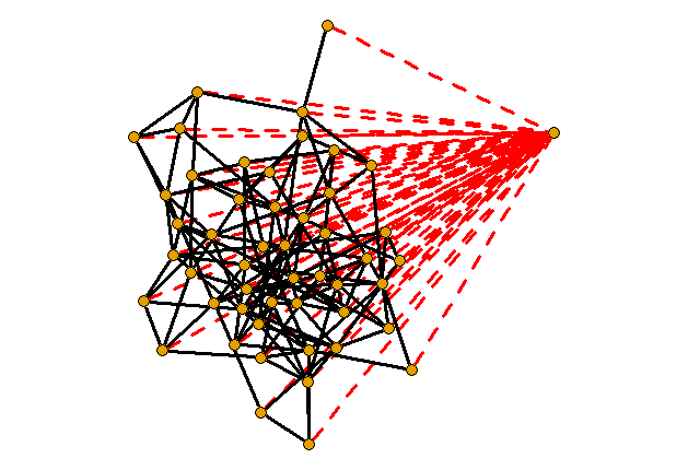
ℳ={(1,p/4+1),…,(1,p/2),(2,p/4+1),…,(p/4,p/2)}.\mathcal{M}=\{(1,p/4+1),\dots,(1,p/2),(2,p/4+1),\dots,(p/4,p/2)\}.
Refer to caption
(a) Random Graph
Refer to caption
(b) Cluster Graph
Fig 1: Examples

The edges of the graph are colored in black and the edges contained in the hypothesis in red.

6.1.3 Example 3: Approximately Sparse Random Graph

In this example we generate a random graph structure as in example 11, but instead of setting the other elements of the adjacency matriy AA to zero we generate independent random entries from a uniform distribution on [−a,a][-a,a] with a=1/20a=1/20. This results in a precision matrix of the form

Φ:=(B0⋮00⋯01)\Phi:=\left(\begin{array}[]{cc}\raisebox{-15.0pt}{{\huge\mbox{{$B$}}}}&0\\[-17.22217pt] &\vdots\\ &0\\ 0\cdots 0&1\end{array}\right)

where BB is not a sparse matrix anymore. We then again test the hypothesis, whether the last regressor is independent from all other regressors, corresponding to

ℳ={(p,1),…,(p,p−1)}.\mathcal{M}=\{(p,1),\dots,(p,p-1)\}.

6.1.4 Example 4: Independent Graph

By setting

Φ:=Ip×p\Phi:=I_{p\times p}

we generate samples of pp independent normal distributed random variables. We can test the hypothesis whether the regressors are independent by choosing

ℳ={(1,2),…,(1,p),(2,3),…,(p−1,p)}.\mathcal{M}=\{(1,2),\dots,(1,p),(2,3),\dots,(p-1,p)\}.

6.2 Simulation results

We provide simulated acceptance rates of our proposed estimation procedure with B=1000B=1000 bootstrap samples for all of the examples above. Confidence Intervall I corresponds to the standard case in (4.2), whereas Confidence Intervall II is based on the approximation of the sphere in (4.3). In summary, the results reveal that the empirical acceptance rate is, on average, close to the nominal level of 95%95\% with a mean absolute deviation of 2.581%2.581\% over all simulations. The Confidence Intervall II has got a mean absolute deviation of 1.875%1.875\% and performs significantly better than Confidence Intervall I with a mean absolute deviation of 3.287%3.287\%. More complex S-sparsely convex sets seem to result in better acceptance rates, whereas higher exponents do not improve the rates. The lowest mean absolute deviation (1.138%1.138\%) is achieved in table 2 for S=5S=5, e​x​p=1exp=1 and without cross-fitting.

Confidence Interval I Confidence Intervall II
Model p d lasso post-lasso sqrt-lasso lasso post-lasso sqrt-lasso
random 20 19 0.931 0.938 0.936 0.929 0.930 0.935
50 49 0.915 0.915 0.916 0.926 0.929 0.932
100 99 0.912 0.912 0.908 0.927 0.930 0.929
cluster 20 25 0.916 0.942 0.918 0.915 0.930 0.921
40 100 0.916 0.919 0.917 0.934 0.947 0.937
60 225 0.897 0.893 0.899 0.921 0.922 0.927
approx 20 19 0.931 0.931 0.931 0.947 0.946 0.947
50 49 0.908 0.908 0.908 0.920 0.920 0.920
100 99 0.902 0.902 0.902 0.935 0.935 0.935
indepent 5 10 0.931 0.931 0.931 0.933 0.933 0.933
10 45 0.927 0.927 0.927 0.937 0.937 0.937
20 190 0.896 0.896 0.896 0.920 0.920 0.920
Table 1: Simulation results for S=1,exp=1 and 1-fold
Confidence Interval I Confidence Intervall II
Model p d lasso post-lasso sqrt-lasso lasso post-lasso sqrt-lasso
random 20 19 0.969 0.925 0.956 0.951 0.932 0.947
50 49 0.942 0.944 0.944 0.942 0.954 0.953
100 99 0.934 0.941 0.940 0.950 0.949 0.952
cluster 20 25 0.972 0.958 0.973 0.914 0.936 0.914
40 100 0.941 0.937 0.945 0.930 0.936 0.942
60 225 0.931 0.947 0.942 0.943 0.937 0.950
approx 20 19 0.958 0.958 0.958 0.965 0.965 0.965
50 49 0.937 0.937 0.937 0.940 0.940 0.940
100 99 0.920 0.921 0.920 0.936 0.936 0.936
indepent 5 10 0.951 0.951 0.951 0.951 0.951 0.951
10 45 0.932 0.932 0.932 0.952 0.952 0.952
20 190 0.926 0.926 0.926 0.947 0.947 0.947
Table 2: Simulation results for S=5,exp=1 and 1-fold
Confidence Interval I Confidence Intervall II
Model p d lasso post-lasso sqrt-lasso lasso post-lasso sqrt-lasso
random 20 19 0.909 0.916 0.921 0.916 0.921 0.930
50 49 0.931 0.910 0.926 0.926 0.907 0.927
100 99 0.907 0.909 0.909 0.917 0.934 0.923
cluster 20 25 0.910 0.905 0.905 0.904 0.898 0.901
40 100 0.909 0.910 0.910 0.905 0.919 0.921
60 225 0.885 0.894 0.898 0.912 0.925 0.934
approx 20 19 0.929 0.928 0.929 0.929 0.928 0.929
50 49 0.888 0.888 0.888 0.911 0.911 0.911
100 99 0.907 0.907 0.907 0.936 0.936 0.936
indepent 5 10 0.930 0.930 0.930 0.939 0.939 0.939
10 45 0.921 0.921 0.921 0.933 0.933 0.933
20 190 0.916 0.916 0.916 0.938 0.938 0.938
Table 3: Simulation results for S=5,exp=2 and 1-fold
Confidence Interval I Confidence Intervall II
Model p d lasso post-lasso sqrt-lasso lasso post-lasso sqrt-lasso
random 20 19 0.917 0.912 0.919 0.919 0.932 0.918
50 49 0.927 0.911 0.925 0.938 0.936 0.938
100 99 0.903 0.894 0.907 0.926 0.933 0.927
cluster 20 25 0.920 0.899 0.918 0.930 0.929 0.929
40 100 0.920 0.883 0.919 0.927 0.926 0.923
60 225 0.889 0.885 0.896 0.920 0.930 0.928
approx 20 19 0.921 0.922 0.921 0.932 0.934 0.932
50 49 0.899 0.899 0.899 0.926 0.926 0.926
100 99 0.889 0.889 0.889 0.930 0.929 0.930
indepent 5 10 0.922 0.923 0.922 0.935 0.934 0.935
10 45 0.905 0.905 0.905 0.937 0.937 0.937
20 190 0.903 0.903 0.903 0.936 0.936 0.936
Table 4: Simulation results for S=1,exp=1 and 3-fold
Confidence Interval I Confidence Intervall II
Model p d lasso post-lasso sqrt-lasso lasso post-lasso sqrt-lasso
random 20 19 0.970 0.919 0.964 0.950 0.932 0.958
50 49 0.923 0.911 0.927 0.938 0.951 0.935
100 99 0.929 0.925 0.930 0.949 0.940 0.948
cluster 20 25 0.971 0.970 0.971 0.915 0.931 0.915
40 100 0.926 0.915 0.925 0.925 0.917 0.924
60 225 0.923 0.925 0.926 0.917 0.939 0.930
approx 20 19 0.959 0.959 0.959 0.958 0.956 0.958
50 49 0.932 0.932 0.932 0.931 0.933 0.931
100 99 0.929 0.929 0.929 0.949 0.950 0.949
indepent 5 10 0.940 0.940 0.940 0.951 0.951 0.951
10 45 0.922 0.922 0.922 0.938 0.938 0.938
20 190 0.930 0.930 0.930 0.938 0.938 0.938
Table 5: Simulation results for S=5,exp=1 and 3-fold
Confidence Interval I Confidence Intervall II
Model p d lasso post-lasso sqrt-lasso lasso post-lasso sqrt-lasso
random 20 19 0.914 0.897 0.918 0.922 0.921 0.923
50 49 0.914 0.896 0.911 0.920 0.920 0.921
100 99 0.891 0.878 0.893 0.918 0.909 0.917
cluster 20 25 0.885 0.882 0.888 0.900 0.896 0.901
40 100 0.880 0.877 0.879 0.898 0.910 0.907
60 225 0.886 0.884 0.897 0.915 0.921 0.932
approx 20 19 0.931 0.930 0.931 0.938 0.937 0.938
50 49 0.914 0.913 0.914 0.932 0.933 0.932
100 99 0.894 0.894 0.894 0.924 0.924 0.924
indepent 5 10 0.923 0.922 0.923 0.943 0.942 0.943
10 45 0.917 0.916 0.917 0.934 0.935 0.934
20 190 0.890 0.890 0.890 0.932 0.932 0.932
Table 6: Simulation results for S=5,exp=2 and 3-fold

A Proof of Theorem 1

We want to use corollary 2.22.2 from Belloni et al. (2018) [2]. Consequently, we will show that their assumptions 2.1-2.4 and the growth conditions of corollary 2.22.2 hold by modifying the proof of corollary 3.23.2 in [2]. To make the proof more comparable we try to keep the notation as similar as possible. This implies that we use CC for a strictly positive constant, independent of nn and rr, which may have a different value in each appearance. The notation an≲bna_{n}\lesssim b_{n} stands for an≤C​bna_{n}\leq Cb_{n} for all nn for some fixed CC. Additionally an=o⁡(1)a_{n}=o(1) stands for uniform convergence towards zero meaning there exists sequence (bn)n≥1(b_{n})_{n\geq 1} with |an|≤bn|a_{n}|\leq b_{n}, bnb_{n} is independent of P∈𝒫nP\in\mathcal{P}_{n} for all nn and bn→0b_{n}\to 0. Finally, the notation an≲Pbna_{n}\lesssim_{P}b_{n} means that for any ϵ>0\epsilon>0, there exists CC such that uniformly over all nn we have PP​(an>C​bn)≤ϵP_{P}(a_{n}>Cb_{n})\leq\epsilon.
Let mr=(j,k)m_{r}=(j,k) be an arbitrary set in ℳ\mathcal{M}. We have

maxr⁡𝔼⁡[(ν(mr))2]≲1​and​maxr⁡𝔼⁡[(ε(mr))2]≲1\max\limits_{r}\mathbb{E}\left[\left(\nu^{(m_{r})}\right)^{2}\right]\lesssim 1\ \text{and}\ \max\limits_{r}\mathbb{E}\left[\left(\varepsilon^{(m_{r})}\right)^{2}\right]\lesssim 1

due to the assumptions A3 and A4. Define the convex set

Tmr={η=(η(1),η(2)):η(1)∈ℝp−2,η(2)∈ℝp−2}T_{m_{r}}=\{\eta=(\eta^{(1)},\eta^{(2)}):\eta^{(1)}\in\mathbb{R}^{p-2},\eta^{(2)}\in\mathbb{R}^{p-2}\}

and endow TmrT_{m_{r}} with the norm

‖η‖e=‖η(1)‖2∨||η(2)||2.||\eta||_{e}=||\eta^{(1)}||_{2}\vee||\eta^{(2)}||_{2}.

Further let τn:=s​log⁡(an)n\tau_{n}:=\sqrt{\frac{s\log(a_{n})}{n}} and define the nuisance realization set

𝒯mr={\displaystyle\mathcal{T}_{m_{r}}=\bigg\{ η∈Tmr:‖η(1)‖0∨‖η(2)‖0≤C​s,\displaystyle\eta\in T_{m_{r}}:||\eta^{(1)}||_{0}\vee||\eta^{(2)}||_{0}\leq Cs,
‖η(1)−β(mr)‖2∨‖η(2)−γ(mr)‖2≤C​τn,\displaystyle||\eta^{(1)}-\beta^{(m_{r})}||_{2}\vee||\eta^{(2)}-\gamma^{(m_{r})}||_{2}\leq C\tau_{n},
||η(1)−β(mr)||1∨||η(2)−γ(mr)||1≤Csτn}∪{(β(mr),γ(mr))}\displaystyle||\eta^{(1)}-\beta^{(m_{r})}||_{1}\vee||\eta^{(2)}-\gamma^{(m_{r})}||_{1}\leq C\sqrt{s}\tau_{n}\bigg\}\cup\left\{\left(\beta^{(m_{r})},\gamma^{(m_{r})}\right)\right\}

for a sufficiently large constant C>0C>0. First we verify Assumption 2.1 (i). The moment condition holds since

𝔼⁡[ψmr​(X,θmr,ηmr)]\displaystyle\hskip 10.00002pt\mathbb{E}[\psi_{m_{r}}(X,\theta_{m_{r}},\eta_{m_{r}})]
=𝔼⁡[ε(mr)​ν(mr)]\displaystyle=\mathbb{E}[\varepsilon^{(m_{r})}\nu^{(m_{r})}]
=𝔼⁡[𝔼⁡[ε(mr)​ν(mr)|X−j]]=𝔼⁡[ν(mr)​𝔼⁡[ε(mr)|X−j]⏟=0]=0.\displaystyle=\mathbb{E}[\mathbb{E}[\varepsilon^{(m_{r})}\nu^{(m_{r})}|X_{-j}]]=\mathbb{E}[\nu^{(m_{r})}\underbrace{\mathbb{E}[\varepsilon^{(m_{r})}|X_{-j}]}_{=0}]=0.

In addition, we have

Sn:\displaystyle S_{n}: =𝔼⁡[maxr⁡|n​𝔼n​[ψmr​(X,θmr,ηmr)]|]\displaystyle=\mathbb{E}\left[\max\limits_{r}|\sqrt{n}\mathbb{E}_{n}[\psi_{m_{r}}(X,\theta_{m_{r}},\eta_{m_{r}})]|\right]
=𝔼⁡[supf∈ℱ𝔾n​(f)]\displaystyle=\mathbb{E}\left[\sup\limits_{f\in\mathcal{F}}\mathbb{G}_{n}(f)\right]

with ℱ={ε(mr)ν(mr)|r=1,…,d}\mathcal{F}=\{\varepsilon^{(m_{r})}\nu^{(m_{r})}|r=1,\dots,d\} and 𝔾n​(f):=n​|𝔼n​[f]−𝔼⁡[f]|\mathbb{G}_{n}(f):=\sqrt{n}|\mathbb{E}_{n}[f]-\mathbb{E}[f]|. By the same arguments as in the beginning of proof of theorem 2 we conclude that the envelope supf∈ℱ|f|\sup\limits_{f\in\mathcal{F}}|f| of ℱ\mathcal{F} fulfills

‖maxr⁡|ε(mr)​ν(mr)|‖P,q\displaystyle||\max\limits_{r}|\varepsilon^{(m_{r})}\nu^{(m_{r})}|||_{P,q} =𝔼​[maxr⁡(|ε(mr)​ν(mr)|)q]1/q\displaystyle=\mathbb{E}\left[\max\limits_{r}\left(|\varepsilon^{(m_{r})}\nu^{(m_{r})}|\right)^{q}\right]^{1/q}
≤𝔼​[maxr⁡(|ε(mr)|)2​q]1/2​q​𝔼​[maxr⁡(|ν(mr)|)2​q]1/2​q\displaystyle\leq\mathbb{E}\left[\max\limits_{r}\left(|\varepsilon^{(m_{r})}|\right)^{2q}\right]^{1/2q}\mathbb{E}\left[\max\limits_{r}\left(|\nu^{(m_{r})}|\right)^{2q}\right]^{1/2q}
≤C​log⁡(d),\displaystyle\leq C\log(d),

since the error terms are normal distributed. Using lemma O.2 (Maximal Inequality I) in [2] with |ℱ|=d|\mathcal{F}|=d, we have

Sn≤C​log1/2⁡(d)+C​log1/2⁡(d)​(n2q​log3⁡(d)n)1/2≲log1/2⁡(d)\displaystyle S_{n}\leq C\log^{1/2}(d)+C\log^{1/2}(d)\left(n^{\frac{2}{q}}\frac{\log^{3}(d)}{n}\right)^{1/2}\lesssim\log^{1/2}(d)

by the assumption A2 for a q>2​q~q>2\tilde{q}. Hence, assumption A3 implies that for all r=1,…,dr=1,\dots,d, Θmr\Theta_{m_{r}} contains an interval of radius C​n−12​Sn​log⁡(n)Cn^{-\frac{1}{2}}S_{n}\log(n) centered at θmr\theta_{m_{r}} for all sufficiently large nn for any constant CC. Assumption 2.1 (i) follows.

For all mr∈ℳm_{r}\in\mathcal{M}, the map (θ,η)↦ψmr​(X,θ,η)(\theta,\eta)\mapsto\psi_{m_{r}}(X,\theta,\eta) is twice continuously Gateaux-differentiable on Θmr×𝒯mr\Theta_{m_{r}}\times\mathcal{T}_{m_{r}}, and so is the map (θ,η)↦𝔼⁡[ψmr​(X,θ,η)](\theta,\eta)\mapsto\mathbb{E}[\psi_{m_{r}}(X,\theta,\eta)]. Further we have

Dmr,0​[η,ηmr]:\displaystyle D_{m_{r},0}[\eta,\eta_{m_{r}}]: =∂t𝔼⁡[ψmr​(X,θmr,ηmr+t⁡(η−ηmr))]|t=0\displaystyle=\partial_{t}\mathbb{E}[\psi_{m_{r}}(X,\theta_{m_{r}},\eta_{m_{r}}+t(\eta-\eta_{m_{r}}))]\big|_{t=0}
=𝔼[∂t{(Xj−θmrXk−(ηmr(1)+t(η(1)−ηmr(1)))X−mr)\displaystyle=\mathbb{E}\bigg[\partial_{t}\bigg\{\left(X_{j}-\theta_{m_{r}}X_{k}-\left(\eta_{m_{r}}^{(1)}+t(\eta^{(1)}-\eta_{m_{r}}^{(1)})\right)X_{-m_{r}}\right)
(Xk−(ηmr(2)+t(η(2)−ηmr(2)))X−mr)}]|t=0\displaystyle\hskip 20.00003pt\left(X_{k}-\left(\eta_{m_{r}}^{(2)}+t(\eta^{(2)}-\eta_{m_{r}}^{(2)})\right)X_{-m_{r}}\right)\bigg\}\bigg]\big|_{t=0}
=𝔼⁡[ε(mr)​(ηmr(2)−η(2))​X−mr]+𝔼⁡[(ηmr(1)−η(1))​X−mr​ν(mr)]\displaystyle=\mathbb{E}[\varepsilon^{(m_{r})}(\eta^{(2)}_{m_{r}}-\eta^{(2)})X_{-m_{r}}]+\mathbb{E}[(\eta_{m_{r}}^{(1)}-\eta^{(1)})X_{-m_{r}}\nu^{(m_{r})}]
=0.\displaystyle=0.

Therefore, Assumptions 2.1 (ii) and 2.1 (iii) hold. Remark that

|Jmr|\displaystyle|J_{m_{r}}| =|∂θ𝔼⁡[ψmr​(X,θ,ηmr)]|θ=θmr|\displaystyle=|\partial_{\theta}\mathbb{E}[\psi_{m_{r}}(X,\theta,\eta_{m_{r}})]|_{\theta=\theta_{m_{r}}}|
=|𝔼⁡[−Xk​ν(mr)]||=|𝔼⁡[(ν(mr))2]|≤C\displaystyle=|\mathbb{E}[-X_{k}\nu^{(m_{r})}]||=|\mathbb{E}[(\nu^{(m_{r})})^{2}]|\leq C

and

|Jmr|\displaystyle|J_{m_{r}}| =|𝔼⁡[(ν(mr))2]|≥c\displaystyle=|\mathbb{E}[(\nu^{(m_{r})})^{2}]|\geq c

due to assumption A4. Since the score ψ\psi is linear with respect to θ\theta, we have for all mr∈ℳm_{r}\in\mathcal{M} and θ∈Θmr\theta\in\Theta_{m_{r}}

𝔼⁡[ψmr​(X,θ,ηmr)]=Jmr​(θ−θmr)\displaystyle\mathbb{E}[\psi_{m_{r}}(X,\theta,\eta_{m_{r}})]=J_{m_{r}}(\theta-\theta_{m_{r}})

using the moment condition. This gives us Assumption 2.1 (iv).
For all t∈[0,1)t\in[0,1), mr∈ℳm_{r}\in\mathcal{M}, θ∈Θmr\theta\in\Theta_{m_{r}}, η∈𝒯mr\eta\in\mathcal{T}_{m_{r}} we have

𝔼⁡[(ψmr​(X,θ,η)−ψmr​(X,θmr,ηmr))2]\displaystyle\mathbb{E}\big[(\psi_{m_{r}}(X,\theta,\eta)-\psi_{m_{r}}(X,\theta_{m_{r}},\eta_{m_{r}}))^{2}\big]
=\displaystyle=\ 𝔼⁡[(ψmr​(X,θ,η)−ψmr​(X,θmr,η)+ψmr​(X,θmr,η)−ψmr​(X,θmr,ηmr))2]\displaystyle\mathbb{E}\big[(\psi_{m_{r}}(X,\theta,\eta)-\psi_{m_{r}}(X,\theta_{m_{r}},\eta)+\psi_{m_{r}}(X,\theta_{m_{r}},\eta)-\psi_{m_{r}}(X,\theta_{m_{r}},\eta_{m_{r}}))^{2}\big]
≤\displaystyle\leq\ C(𝔼⁡[(ψmr​(X,θ,η)−ψmr​(X,θmr,η))2]⏟=:I\displaystyle C\bigg(\underbrace{\mathbb{E}\big[(\psi_{m_{r}}(X,\theta,\eta)-\psi_{m_{r}}(X,\theta_{m_{r}},\eta))^{2}\big]}_{=:I}
∨𝔼⁡[(ψmr​(X,θmr,η)−ψmr​(X,θmr,ηmr))2]⏟=:I​I)\displaystyle\hskip 10.00002pt\vee\underbrace{\mathbb{E}\big[(\psi_{m_{r}}(X,\theta_{m_{r}},\eta)-\psi_{m_{r}}(X,\theta_{m_{r}},\eta_{m_{r}}))^{2}\big]}_{=:II}\bigg)

with

I\displaystyle I =|θ−θmr|2​𝔼​[(Xk​(Xk−η(2)​X−mr))2]\displaystyle=|\theta-\theta_{m_{r}}|^{2}\mathbb{E}\left[\left(X_{k}(X_{k}-\eta^{(2)}X_{-m_{r}})\right)^{2}\right]
≤|θ−θmr|2​(𝔼⁡[Xk2]​E​[(Xk−η(2)​X−mr)2])1/2\displaystyle\leq|\theta-\theta_{m_{r}}|^{2}\left(\mathbb{E}[X_{k}^{2}]E[(X_{k}-\eta^{(2)}X_{-m_{r}})^{2}]\right)^{1/2}
≤C​|θ−θmr|2\displaystyle\leq C|\theta-\theta_{m_{r}}|^{2}

due to assumptions A3, A4 and the definition of 𝒯mr\mathcal{T}_{m_{r}}. Additionally we have

I​I\displaystyle II =𝔼[((Xj−θmrXk−η(1)X−mr)(Xk−η(2)X−mr)\displaystyle=\mathbb{E}\bigg[\Big(\big(X_{j}-\theta_{m_{r}}X_{k}-\eta^{(1)}X_{-m_{r}}\big)\big(X_{k}-\eta^{(2)}X_{-m_{r}}\big)
−(Xj−θmrXk−ηmr(1)X−mr)(Xk−ηmr(2)X−mr))2]\displaystyle\hskip 10.00002pt\hskip 10.00002pt-\big(X_{j}-\theta_{m_{r}}X_{k}-\eta^{(1)}_{m_{r}}X_{-m_{r}}\big)\big(X_{k}-\eta^{(2)}_{m_{r}}X_{-m_{r}}\big)\Big)^{2}\bigg]
=𝔼[((Xj−θmrXk−η(1)X−mr)((ηmr(2)−η(2))X−mr)\displaystyle=\mathbb{E}\bigg[\Big(\big(X_{j}-\theta_{m_{r}}X_{k}-\eta^{(1)}X_{-m_{r}}\big)\big((\eta^{(2)}_{m_{r}}-\eta^{(2)})X_{-m_{r}}\big)
+(Xk−ηmr(2)X−mr)((ηmr(1)−η(1))X−mr))2]\displaystyle\hskip 10.00002pt\hskip 10.00002pt+\big(X_{k}-\eta^{(2)}_{m_{r}}X_{-m_{r}}\big)\big((\eta^{(1)}_{m_{r}}-\eta^{(1)})X_{-m_{r}}\big)\Big)^{2}\bigg]
≤C​(‖ηmr(2)−η(2)‖2∨‖ηmr(1)−η(1)‖2)2\displaystyle\leq C\Big(\|\eta^{(2)}_{m_{r}}-\eta^{(2)}\|_{2}\vee\|\eta^{(1)}_{m_{r}}-\eta^{(1)}\|_{2}\Big)^{2}
=C​‖ηmr−η‖e2\displaystyle=C\|\eta_{m_{r}}-\eta\|_{e}^{2}

with similar arguments as in II above using

sup‖ξ‖2=1𝔼⁡[(ξ​X)4]≤C\sup\limits_{\|\xi\|_{2}=1}\mathbb{E}\left[(\xi X)^{4}\right]\leq C

due to the normal distributed design. Combining these results gives us Assumption 2.1 (v) (a).
Observe that

|∂t𝔼⁡[ψmr​(X,θ,ηmr+t⁡(η−ηmr))]|\displaystyle\ \Big|\partial_{t}\mathbb{E}\Big[\psi_{m_{r}}\big(X,\theta,\eta_{m_{r}}+t(\eta-\eta_{m_{r}})\big)\Big]\Big|
=\displaystyle= |𝔼[(Xj−θXk−(ηmr(1)+t(η(1)−ηmr(1)))X−mr)((ηmr(2)−η(2))X−mr)\displaystyle\ \bigg|\mathbb{E}\bigg[\Big(X_{j}-\theta X_{k}-\big(\eta^{(1)}_{m_{r}}+t(\eta^{(1)}-\eta^{(1)}_{m_{r}})\big)X_{-m_{r}}\Big)\big((\eta^{(2)}_{m_{r}}-\eta^{(2)})X_{-m_{r}}\big)
+(Xk−(ηmr(2)+t(η(2)−ηmr(2)))X−mr)((ηmr(1)−η(1))X−mr)]|\displaystyle\hskip 10.00002pt\hskip 10.00002pt+\Big(X_{k}-\big(\eta^{(2)}_{m_{r}}+t(\eta^{(2)}-\eta^{(2)}_{m_{r}})\big)X_{-m_{r}}\Big)\big((\eta^{(1)}_{m_{r}}-\eta^{(1)})X_{-m_{r}}\big)\bigg]\bigg|
≤\displaystyle\leq C​‖ηmr−η‖e\displaystyle\ C\|\eta_{m_{r}}-\eta\|_{e}

with the same argument as above, which gives us Assumption 2.1 (v) (b) with B1​n=CB_{1n}=C. To complete the Assumption 2.1 (v) (c) with B2​n=CB_{2n}=C observe that

|∂t2𝔼⁡[ψmr​(X,θmr+t⁡(θ−θmr),ηmr+t⁡(η−ηmr))]|\displaystyle\Big|\partial^{2}_{t}\mathbb{E}\Big[\psi_{m_{r}}\big(X,\theta_{m_{r}}+t(\theta-\theta_{m_{r}}),\eta_{m_{r}}+t(\eta-\eta_{m_{r}})\big)\Big]\Big|
=\displaystyle= |∂t𝔼[(Xj−(θmr+t(θ−θmr))Xk−(ηmr(1)+t(η(1)−ηmr(1)))X−mr)\displaystyle\bigg|\partial_{t}\mathbb{E}\bigg[\Big(X_{j}-\big(\theta_{m_{r}}+t(\theta-\theta_{m_{r}})\big)X_{k}-\big(\eta^{(1)}_{m_{r}}+t(\eta^{(1)}-\eta^{(1)}_{m_{r}})\big)X_{-m_{r}}\Big)
⋅((ηmr(2)−η(2))​X−mr)\displaystyle\hskip 10.00002pt\hskip 10.00002pt\cdot\big((\eta^{(2)}_{m_{r}}-\eta^{(2)})X_{-m_{r}}\big)
+(Xk−(ηmr(2)+t⁡(η(2)−ηmr(2)))​X−mr)\displaystyle\hskip 10.00002pt\hskip 10.00002pt+\Big(X_{k}-\big(\eta^{(2)}_{m_{r}}+t(\eta^{(2)}-\eta^{(2)}_{m_{r}})\big)X_{-m_{r}}\Big)
⋅((θmr−θ)Xk+(ηmr(1)−η(1))X−mr)]|\displaystyle\hskip 10.00002pt\hskip 10.00002pt\cdot\big((\theta_{m_{r}}-\theta)X_{k}+(\eta^{(1)}_{m_{r}}-\eta^{(1)})X_{-m_{r}}\big)\bigg]\bigg|
=\displaystyle= |2​𝔼​[((ηmr(2)−η(2))​X−mr)​((θmr−θ)​Xk+(ηmr(1)−η(1))​X−mr)]|\displaystyle\Big|2\mathbb{E}\Big[\big((\eta^{(2)}_{m_{r}}-\eta^{(2)})X_{-m_{r}}\big)\big((\theta_{m_{r}}-\theta)X_{k}+(\eta^{(1)}_{m_{r}}-\eta^{(1)})X_{-m_{r}}\big)\Big]\Big|
≤\displaystyle\leq 2​(𝔼⁡[((ηmr(2)−η(2))​X−mr)2]⏟≤C​‖ηmr(2)−η(2)‖22​𝔼⁡[((θmr−θ)​Xk+(ηmr(1)−η(1))​X−mr)2]⏟≤C⁡(|θmr−θ|2+‖ηmr(1)−η(1)‖22))1/2\displaystyle\ 2\bigg(\underbrace{\mathbb{E}\Big[\big((\eta^{(2)}_{m_{r}}-\eta^{(2)})X_{-m_{r}}\big)^{2}\Big]}_{\leq C\|\eta^{(2)}_{m_{r}}-\eta^{(2)}\|_{2}^{2}}\underbrace{\mathbb{E}\Big[\big((\theta_{m_{r}}-\theta)X_{k}+(\eta^{(1)}_{m_{r}}-\eta^{(1)})X_{-m_{r}}\big)^{2}\Big]}_{\leq C\big(|\theta_{m_{r}}-\theta|^{2}+\|\eta^{(1)}_{m_{r}}-\eta^{(1)}\|_{2}^{2}\big)}\bigg)^{1/2}
≤\displaystyle\leq C⁡(|θmr−θ|2∨‖ηmr−η‖e2).\displaystyle\ C\big(|\theta_{m_{r}}-\theta|^{2}\vee\|\eta_{m_{r}}-\eta\|_{e}^{2}\big).

Therefore Assumption 2.1 holds. Due to the construction of 𝒯mr\mathcal{T}_{m_{r}} Assumptions 2.2 (ii) and (iii) hold. Next, we show that the assumptions of theorem 2 from section B hold which implies Assumption 2.2 (i). Remark that conditions B1 and B4 are satisfied with ρ=2\rho=2. Condition A1 implies condition B3. Let σ¯2>0\underline{\sigma}^{2}>0 be a uniform lower bound for the variances of the error terms and the regressors and let c:=σ¯​zc~c:=\underline{\sigma}z_{\tilde{c}}, where zc~z_{\tilde{c}} is the c~\tilde{c}-quantile of a standard normal distribution for an arbitrary but fixed c~∈(12,34)\tilde{c}\in(\frac{1}{2},\frac{3}{4}). Uniformly for all r=1,…,dr=1,\dots,d and l∈{1,…,p}∖{j}l\in\{1,\dots,p\}\setminus\{j\}, it holds

P⁡((ε(mr))2​Xl2≥c4)\displaystyle P\left((\varepsilon^{(m_{r})})^{2}X_{l}^{2}\geq c^{4}\right) =1−P⁡(|ε(mr)​Xl|≤c2)\displaystyle=1-P\left(|\varepsilon^{(m_{r})}X_{l}|\leq c^{2}\right)
≥1−P⁡(|ε(mr)|≤c∨|Xl|≤c)\displaystyle\geq 1-P\left(|\varepsilon^{(m_{r})}|\leq c\vee|X_{l}|\leq c\right)
≥1−(P⁡(|ε(mr)|≤c)+P⁡(|Xl|≤c))\displaystyle\geq 1-\left(P\left(|\varepsilon^{(m_{r})}|\leq c\right)+P\left(|X_{l}|\leq c\right)\right)
≥1−2​P​(σ¯​|Z|≤c)\displaystyle\geq 1-2P\left(\underline{\sigma}|Z|\leq c\right)
=3−4​c~>0\displaystyle=3-4\tilde{c}>0

where Z∼𝒩⁡(0,1)Z\sim\mathcal{N}(0,1), which implies that

minr⁡minl⁡𝔼⁡[(ε(mr))2​Xl2]\displaystyle\min_{r}\min_{l}\mathbb{E}[(\varepsilon^{(m_{r})})^{2}X_{l}^{2}] ≥c4​(3−4​c~)>0.\displaystyle\geq c^{4}(3-4\tilde{c})>0.

Analogously

minr⁡minl⁡𝔼⁡[(ν(mr))2​Xl2]>0.\displaystyle\min_{r}\min_{l}\mathbb{E}[(\nu^{(m_{r})})^{2}X_{l}^{2}]>0.

Combined with condition A4 this implies condition B2. Therefore we are able to estimate the nuisance parameters at a sufficiently fast rate.
Define

ℱ1:\displaystyle\mathcal{F}_{1}: ={ψmr(⋅,θ,η):r∈{1,…,d},θ∈Θmr,η∈𝒯mr}.\displaystyle=\Big\{\psi_{m_{r}}(\cdot,\theta,\eta):r\in\{1,\dots,d\},\theta\in\Theta_{m_{r}},\eta\in\mathcal{T}_{m_{r}}\Big\}.

To bound the covering entropy of ℱ1\mathcal{F}_{1} we at first exclude the true nuisance parameter and define

ℱ1,1:\displaystyle\mathcal{F}_{1,1}: ={ψmr(⋅,θ,η):r∈{1,…,d},θ∈Θmr,η∈𝒯mr∖{ηmr}}⊆ℱ1,1(1)ℱ1,1(2)\displaystyle=\Big\{\psi_{m_{r}}(\cdot,\theta,\eta):r\in\{1,\dots,d\},\theta\in\Theta_{m_{r}},\eta\in\mathcal{T}_{m_{r}}\setminus\{\eta_{m_{r}}\}\Big\}\subseteq\mathcal{F}_{1,1}^{(1)}\mathcal{F}_{1,1}^{(2)}

with

ℱ1,1(1)\displaystyle\mathcal{F}_{1,1}^{(1)} ={X→(Xj−θXk−η(1)X−mr):r∈{1,…,d},θ∈Θmr,η(1)∈𝒯mr,1∗}\displaystyle=\{X\to(X_{j}-\theta X_{k}-\eta^{(1)}X_{-m_{r}}):r\in\{1,\dots,d\},\theta\in\Theta_{m_{r}},\eta^{(1)}\in\mathcal{T}^{*}_{m_{r},1}\}
ℱ1,1(2)\displaystyle\mathcal{F}_{1,1}^{(2)} ={X→(Xk−η(2)X−mr):r∈{1,…,d},η(2)∈𝒯mr,2∗}\displaystyle=\{X\to(X_{k}-\eta^{(2)}X_{-m_{r}}):r\in\{1,\dots,d\},\eta^{(2)}\in\mathcal{T}^{*}_{m_{r},2}\}

where 𝒯mr∗:=𝒯mr∖{ηmr}\mathcal{T}^{*}_{m_{r}}:=\mathcal{T}_{m_{r}}\setminus\{\eta_{m_{r}}\}. Observe that the envelope F1,1(1)F_{1,1}^{(1)} of ℱ1,1(1)\mathcal{F}_{1,1}^{(1)} fulfills

‖(F1,1(1))2‖P,2​q\displaystyle\big\|\big(F_{1,1}^{(1)}\big)^{2}\big\|_{P,2q} ≤|supr∈{1,…,d}supθ∈Θmr,‖ηmr(1)−η(1)‖1≤C​s​τn(|ε(mr)|CLOSE\displaystyle\leq\Big\|\sup\limits_{r\in\{1,\dots,d\}}\sup\limits_{\theta\in\Theta_{m_{r}},\|\eta^{(1)}_{m_{r}}-\eta^{(1)}\|_{1}\leq C\sqrt{s}\tau_{n}}\Big(|\varepsilon^{(m_{r})}|
+|(θmr−θ)Xk|+|(ηmr(1)−η(1))X−mr|)2∥P,2​q\displaystyle\hskip 10.00002pt\hskip 10.00002pt+|(\theta_{m_{r}}-\theta)X_{k}|+|(\eta^{(1)}_{m_{r}}-\eta^{(1)})X_{-m_{r}}|\Big)^{2}\Big\|_{P,2q}
≲‖supr∈{1,…,d}(ε(mr))2‖P,2​q+‖supr∈{1,…,d}Xk2‖P,2​q\displaystyle\lesssim\big\|\sup\limits_{r\in\{1,\dots,d\}}\big(\varepsilon^{(m_{r})}\big)^{2}\big\|_{P,2q}+\big\|\sup\limits_{r\in\{1,\dots,d\}}X_{k}^{2}\big\|_{P,2q}
+s​τn2​‖supr∈{1,…,d}‖X−mr‖∞2‖P,2​q\displaystyle\hskip 10.00002pt\hskip 10.00002pt+s\tau_{n}^{2}\big\|\sup\limits_{r\in\{1,\dots,d\}}\|X_{-m_{r}}\|^{2}_{\infty}\big\|_{P,2q}
≲log⁡(d)+log⁡(d)+s​τn2​log⁡(an)\displaystyle\lesssim\log(d)+\log(d)+s\tau_{n}^{2}\log(a_{n})
≲log⁡(an)\displaystyle\lesssim\log(a_{n})

and with an analogous argument

‖(F1,1(2))2‖P,2​q≲log⁡(an).\big\|\big(F_{1,1}^{(2)}\big)^{2}\big\|_{P,2q}\lesssim\log(a_{n}).

Since we excluded the true nuisance parameter, which does not need to be sparse, we have ℱ1,1(1)⊆𝒢1,1\mathcal{F}_{1,1}^{(1)}\subseteq\mathcal{G}_{1,1} and ℱ1,1(2)⊆𝒢1,1\mathcal{F}_{1,1}^{(2)}\subseteq\mathcal{G}_{1,1} with

𝒢1,1:={X→ξX:ξ∈ℝp,∥ξ∥0≤Cs,∥ξ∥2≤C}\mathcal{G}_{1,1}:=\Big\{X\to\xi X:\xi\in\mathbb{R}^{p},\|\xi\|_{0}\leq Cs,\|\xi\|_{2}\leq C\Big\}

where 𝒢1,1\mathcal{G}_{1,1} is a union over (pC​s){p}\choose{Cs} VC-subgraph classes 𝒢1,1,k\mathcal{G}_{1,1,k} with VC indices less or equal to C​s+2Cs+2 (Lemma 2.6.15, Van der Vaart and Wellner (1996)[17]). This implies that ℱ1,1(1)\mathcal{F}_{1,1}^{(1)} and ℱ1,1(2)\mathcal{F}_{1,1}^{(2)} are unions over (pC​s){p}\choose{Cs} VC-subgraph classes ℱ1,1,k(1)\mathcal{F}_{1,1,k}^{(1)} and ℱ1,1,k(2)\mathcal{F}_{1,1,k}^{(2)} with VC indices less or equal to C​s+2Cs+2.
Due to theorem 2.6.7 in [17] we obtain

supQlogN(ε∥F1,1(1)∥Q,2,ℱ1,1(1),∥⋅∥Q,2)\displaystyle\hskip 10.00002pt\sup_{Q}\log N(\varepsilon\|F_{1,1}^{(1)}\|_{Q,2},\mathcal{F}_{1,1}^{(1)},\|\cdot\|_{Q,2})
≤supQlog(∑k=1(pC​s)N(ε∥F1,1(1)∥Q,2,ℱ1,1,k(1),∥⋅∥Q,2))\displaystyle\leq\sup_{Q}\log\Bigg(\sum\limits_{k=1}^{\binom{p}{Cs}}N(\varepsilon\|F_{1,1}^{(1)}\|_{Q,2},\mathcal{F}_{1,1,k}^{(1)},\|\cdot\|_{Q,2})\Bigg)
≤log⁡((pC​s)⏟≤(e⋅pC​s)C​s​K​(C​s+2)​(16​e)C​s+2​(1ε)2​C​s+2)\displaystyle\leq\log\Bigg(\underbrace{\binom{p}{Cs}}_{\leq\big(\frac{e\cdot p}{Cs}\big)^{Cs}}K(Cs+2)(16e)^{Cs+2}\left(\frac{1}{\varepsilon}\right)^{2Cs+2}\Bigg)
≤log⁡((e⋅pC​s)C​s​K​(C​s+2)​(16​e)C​s+2​(1ε)2​C​s+2)\displaystyle\leq\log\Bigg(\left(\frac{e\cdot p}{Cs}\right)^{Cs}K(Cs+2)(16e)^{Cs+2}\left(\frac{1}{\varepsilon}\right)^{2Cs+2}\Bigg)
≲s​log⁡(anε)\displaystyle\lesssim s\log\Big(\frac{a_{n}}{\varepsilon}\Big)

where KK is an universal constant and with an analogous argument

supQlogN(ε∥F1,1(2)∥Q,2,ℱ1,1(2),∥⋅∥Q,2)≲slog(anε).\hskip 10.00002pt\sup_{Q}\log N(\varepsilon\|F_{1,1}^{(2)}\|_{Q,2},\mathcal{F}_{1,1}^{(2)},\|\cdot\|_{Q,2})\lesssim s\log\Big(\frac{a_{n}}{\varepsilon}\Big).

Using basic calculations on covering entropies (see for example Appendix N Lemma N.1 from Belloni et al. (2014) [3]) we can bound the covering entropy of the class ℱ1,1\mathcal{F}_{1,1} by

supQlogN(ε∥F1,1(1)F1,1(2)∥Q,2,ℱ1,1,∥⋅∥Q,2)\displaystyle\sup_{Q}\log N(\varepsilon\|F_{1,1}^{(1)}F_{1,1}^{(2)}\|_{Q,2},\mathcal{F}_{1,1},\|\cdot\|_{Q,2})
≤\displaystyle\leq\hskip 10.00002pt supQlogN(ε2∥F1,1(1)∥Q,2,ℱ1,1(1),∥⋅∥Q,2)\displaystyle\sup_{Q}\log N\Big(\frac{\varepsilon}{2}\|F_{1,1}^{(1)}\|_{Q,2},\mathcal{F}_{1,1}^{(1)},\|\cdot\|_{Q,2}\Big)
+supQlogN(ε2∥F1,1(2)∥Q,2,ℱ1,1(2),∥⋅∥Q,2)\displaystyle\hskip 10.00002pt+\sup_{Q}\log N\Big(\frac{\varepsilon}{2}\|F_{1,1}^{(2)}\|_{Q,2},\mathcal{F}_{1,1}^{(2)},\|\cdot\|_{Q,2}\Big)
≲\displaystyle\lesssim\hskip 10.00002pt s​log⁡(anε)\displaystyle s\log\Big(\frac{a_{n}}{\varepsilon}\Big)

where F1,1:=F1,1(1)​F1,1(2)F_{1,1}:=F_{1,1}^{(1)}F_{1,1}^{(2)} is an envelope for ℱ1,1\mathcal{F}_{1,1} with

‖F1,1‖P,q≤(‖(F1,1(1))2‖P,2​q​‖(F1,1(1))2‖P,2​q)1/2≲log⁡(an).\|F_{1,1}\|_{P,q}\leq\Big(\big\|\big(F_{1,1}^{(1)}\big)^{2}\big\|_{P,2q}\big\|\big(F_{1,1}^{(1)}\big)^{2}\big\|_{P,2q}\Big)^{1/2}\lesssim\log(a_{n}).

Additionally define

ℱ1,2:\displaystyle\mathcal{F}_{1,2}: ={ψmr(⋅,θ,ηmr):r∈{1,…,d},θ∈Θmr}.\displaystyle=\Big\{\psi_{m_{r}}(\cdot,\theta,\eta_{m_{r}}):r\in\{1,\dots,d\},\theta\in\Theta_{m_{r}}\Big\}.

With the same argument as above ℱ1,2\mathcal{F}_{1,2} is a union over dd VC-subgraph classes with VC indices less or equal to 33 implying

supQlogN(ε∥F1,2∥Q,2,ℱ1,2,∥⋅∥Q,2)≤Clog(dε)≲log(anε)\displaystyle\sup_{Q}\log N(\varepsilon\|F_{1,2}\|_{Q,2},\mathcal{F}_{1,2},\|\cdot\|_{Q,2})\leq C\log\Big(\frac{d}{\varepsilon}\Big)\lesssim\log\Big(\frac{a_{n}}{\varepsilon}\Big)

where the envelope F1,2F_{1,2} of ℱ1,2\mathcal{F}_{1,2} obeys

‖F1,2‖P,q≲log⁡(an)\displaystyle\|F_{1,2}\|_{P,q}\lesssim\log(a_{n})

with an analogous argument as above. Combining these results we obtain

supQlogN(ε∥F1∥Q,2,ℱ1,∥⋅∥Q,2)\displaystyle\sup_{Q}\log N(\varepsilon\|F_{1}\|_{Q,2},\mathcal{F}_{1},\|\cdot\|_{Q,2})
=\displaystyle= supQlogN(ε∥F1,1(1)F1,1(2)∨F1,2∥Q,2,ℱ1,1∪ℱ1,2,∥⋅∥Q,2)\displaystyle\hskip 10.00002pt\sup_{Q}\log N(\varepsilon\|F_{1,1}^{(1)}F_{1,1}^{(2)}\vee F_{1,2}\|_{Q,2},\mathcal{F}_{1,1}\cup\mathcal{F}_{1,2},\|\cdot\|_{Q,2})
≤\displaystyle\leq supQlogN(ε∥F1,1(1)F1,1(2)∥Q,2,ℱ1,1,∥⋅∥Q,2)\displaystyle\hskip 10.00002pt\sup_{Q}\log N(\varepsilon\|F_{1,1}^{(1)}F_{1,1}^{(2)}\|_{Q,2},\mathcal{F}_{1,1},\|\cdot\|_{Q,2})
+supQlogN(ε∥F1,2∥Q,2,ℱ1,2,∥⋅∥Q,2)\displaystyle\hskip 10.00002pt\hskip 10.00002pt+\sup_{Q}\log N(\varepsilon\|F_{1,2}\|_{Q,2},\mathcal{F}_{1,2},\|\cdot\|_{Q,2})
≲\displaystyle\lesssim s​log⁡(anε)\displaystyle\hskip 10.00002pts\log\Big(\frac{a_{n}}{\varepsilon}\Big)

where the envelope F1:=F1,1(1)​F1,1(2)∨F1,2F_{1}:=F_{1,1}^{(1)}F_{1,1}^{(2)}\vee F_{1,2} of ℱ1\mathcal{F}_{1} satisfies

‖F1‖P,q≲log⁡(an)\|F_{1}\|_{P,q}\lesssim\log(a_{n})

which gives us Assumption 2.2 (iv). Observe that for all f∈ℱ1f\in\mathcal{F}_{1} we have

𝔼​[f2]1/2\displaystyle\mathbb{E}[f^{2}]^{1/2} ≤supr,θ,η(1)𝔼​[(Xj−θ​Xk−η(1)​X−mr)4]1/4​supr,η(2)𝔼​[(Xk−η(2)​X−mr)4]1/4\displaystyle\leq\sup\limits_{r,\theta,\eta^{(1)}}\mathbb{E}\left[(X_{j}-\theta X_{k}-\eta^{(1)}X_{-m_{r}})^{4}\right]^{1/4}\sup\limits_{r,\eta^{(2)}}\mathbb{E}\left[(X_{k}-\eta^{(2)}X_{-m_{r}})^{4}\right]^{1/4}
≲sup‖ξ‖2=1𝔼​[(ξ​X)4]1/2≲C\displaystyle\lesssim\sup\limits_{\|\xi\|_{2}=1}\mathbb{E}\left[(\xi X)^{4}\right]^{1/2}\lesssim C

and

𝔼[f2]1/2=𝔼[(Xj−θ​Xk−η(1)​X−mr⏟=:Z1)2(Xk−η(2)​X−mr⏟=:Z2)2]1/2.\mathbb{E}[f^{2}]^{1/2}=\mathbb{E}\Big[(\underbrace{X_{j}-\theta X_{k}-\eta^{(1)}X_{-m_{r}}}_{=:Z_{1}})^{2}(\underbrace{X_{k}-\eta^{(2)}X_{-m_{r}}}_{=:Z_{2}})^{2}\Big]^{1/2}.

For each ZiZ_{i} with i∈{1,2}i\in\{1,2\} we have

E⁡[Zi2]≳inf‖ξ‖2=1𝔼⁡[(ξ​X)2]≥c.E[Z_{i}^{2}]\gtrsim\inf\limits_{\|\xi\|_{2}=1}\mathbb{E}\left[(\xi X)^{2}\right]\geq c.

Therefore Z1Z_{1} and Z2Z_{2} are both centered normal distributed random variables where the variance is bounded away from zero. This implies

E​[Z12​Z22]1/2≥c>0E[Z_{1}^{2}Z_{2}^{2}]^{1/2}\geq c>0

which gives us Assumption 2.2 (v).
Assumption 2.2 (vi) (a) holds by construction of τn\tau_{n} and vn≲sv_{n}\lesssim s. Due to the growth condition A2 we can choose q=2​q~/(1−κ)q=2\tilde{q}/(1-\kappa) such that

n−1/2+1/qslog2(an)\displaystyle n^{-1/2+1/q}s\log^{2}(a_{n}) =n1−κ2​q~n−1/2slog2(an)\displaystyle=n^{\frac{1-\kappa}{2\tilde{q}}}n^{-1/2}s\log^{2}(a_{n})
=n−κ2​q~​(n1q~​s2​log4⁡(an)n)1/2≲n−κ2​q~.\displaystyle=n^{-\frac{\kappa}{2\tilde{q}}}\left(n^{\frac{1}{\tilde{q}}}\frac{s^{2}\log^{4}(a_{n})}{n}\right)^{1/2}\lesssim n^{-\frac{\kappa}{2\tilde{q}}}.

Additionally we have

C​τn​(s​log⁡(an))1/2≲s​log⁡(an)n≲n−12​q~,\displaystyle C\tau_{n}(s\log(a_{n}))^{1/2}\lesssim\frac{s\log(a_{n})}{\sqrt{n}}\lesssim n^{-\frac{1}{2\tilde{q}}},
log1/2⁡(d)​log⁡(n)n​(s​log⁡(an))1/2≲s​log4​(an)n≲n−12​q~\displaystyle\log^{1/2}(d)\frac{\log(n)}{\sqrt{n}}(s\log(a_{n}))^{1/2}\lesssim\sqrt{\frac{s\log^{4}(a_{n})}{n}}\lesssim n^{-\frac{1}{2\tilde{q}}}

and

n1/2​τn2=s​log⁡(an)n≲n−12​q~n^{1/2}\tau_{n}^{2}=\frac{s\log(a_{n})}{\sqrt{n}}\lesssim n^{-\frac{1}{2\tilde{q}}}

which gives us Assumption 2.2 (vi) (b) and (c) with δn=n−κ2​q~\delta_{n}=n^{-\frac{\kappa}{2\tilde{q}}}. Define the class

ℱ0:={ψ¯mr(⋅):r=1,…,d}\mathcal{F}_{0}:=\{\bar{\psi}_{m_{r}}(\cdot):r=1,\dots,d\}

where ψ¯mr​(⋅):=−σmr−1​Jmr−1​ψmr​(⋅,θmr,ηmr)\bar{\psi}_{m_{r}}(\cdot):=-\sigma_{m_{r}}^{-1}J_{m_{r}}^{-1}\psi_{m_{r}}(\cdot,\theta_{m_{r}},\eta_{m_{r}}) with σmr2:=Jmr−2​𝔼​[ψmr2​(X,θmr,ηmr)]\sigma_{m_{r}}^{2}:=J_{m_{r}}^{-2}\mathbb{E}[\psi_{m_{r}}^{2}(X,\theta_{m_{r}},\eta_{m_{r}})]. Observe that by the Cauchy-Schwarz Inequality for any q>0q>0 the envelope F0F_{0} for ℱ0\mathcal{F}_{0} satisfies

‖F0‖P,q\displaystyle\|F_{0}\|_{P,q} =𝔼[supr=1,…,d(𝔼[(ε(mr)ν(mr))2]−1/2|ε(mr)ν(mr)|)q]1/q\displaystyle=\mathbb{E}\left[\sup\limits_{r=1,\dots,d}\Big(\mathbb{E}[(\varepsilon^{(m_{r})}\nu^{(m_{r})})^{2}]^{-1/2}|\varepsilon^{(m_{r})}\nu^{(m_{r})}|\Big)^{q}\right]^{1/q}
≲𝔼​[supr=1,…,d(|ε(mr)​ν(mr)|)q]1/q\displaystyle\lesssim\mathbb{E}\left[\sup\limits_{r=1,\dots,d}\big(|\varepsilon^{(m_{r})}\nu^{(m_{r})}|\big)^{q}\right]^{1/q}
≲log⁡(d).\displaystyle\lesssim\log(d).

Since |ℱ0|=d|\mathcal{F}_{0}|=d we have

supQlogN(ε∥F0∥Q,2,ℱ0,∥⋅∥Q,2)≤log(dε)\sup\limits_{Q}\log N\big(\varepsilon\|F_{0}\|_{Q,2},\mathcal{F}_{0},\|\cdot\|_{Q,2}\big)\leq\log\Big(\frac{d}{\varepsilon}\Big)

for all <ε≤1<\varepsilon\leq 1. Therefore Assumption 2.3 (i) is satisfied with ϱn=1\varrho_{n}=1 and An=d∨nA_{n}=d\vee n. Since the errors are centered normal distributed random variables with a uniformly bounded variance we have E⁡[(ε(mr))8]≲CE\big[\big(\varepsilon^{(m_{r})}\big)^{8}\big]\lesssim C and E⁡[(ν(mr))8]≲CE\big[\big(\nu^{(m_{r})}\big)^{8}\big]\lesssim C. This implies 𝔼⁡[f4]≤C\mathbb{E}[f^{4}]\leq C for all f∈ℱ0f\in\mathcal{F}_{0} which gives us Assumption 2.3 (ii). The growth condititons from corollary 2.12.1 are satisfied due to Condition A2. Observe that

δn2​log⁡(n∨d)≲n−κq~​log⁡(n∨d)=o⁡(1),\delta_{n}^{2}\log(n\vee d)\lesssim n^{-\frac{\kappa}{\tilde{q}}}\log(n\vee d)=o(1),
log2/7⁡(d)​log⁡(n∨d)=o⁡(n1/7)\log^{2/7}(d)\log(n\vee d)=o(n^{1/7})

and we can find a qq such that

log2/3⁡(d)​log⁡(n∨d)=o⁡(n1/3−2/(3​q)).\log^{2/3}(d)\log(n\vee d)=o(n^{1/3-2/(3q)}).

Now, we verify Assumption 2.4. Define

ψ~mr​(X,η(2)):\displaystyle\tilde{\psi}_{m_{r}}(X,\eta^{(2)}): =−Xk​(Xk−η(2)​X−mr)\displaystyle=-X_{k}(X_{k}-\eta^{(2)}X_{-m_{r}})

and

m~mr​(η(2)):\displaystyle\tilde{m}_{m_{r}}(\eta^{(2)}): =𝔼⁡[ψ~mr​(X,η(2))],\displaystyle=\mathbb{E}[\tilde{\psi}_{m_{r}}(X,\eta^{(2)})],

where J^mr=−𝔼n​[ψ~mr​(X,η^(2))]\hat{J}_{m_{r}}=-\mathbb{E}_{n}[\tilde{\psi}_{m_{r}}(X,\hat{\eta}^{(2)})]. It holds

|J^mr−Jmr|≤|J^mr−m~mr​(η^(2))|+|m~mr​(η^(2))−m~mr​(ηmr(2))|\displaystyle|\hat{J}_{m_{r}}-J_{m_{r}}|\leq|\hat{J}_{m_{r}}-\tilde{m}_{m_{r}}(\hat{\eta}^{(2)})|+|\tilde{m}_{m_{r}}(\hat{\eta}^{(2)})-\tilde{m}_{m_{r}}(\eta^{(2)}_{m_{r}})|

with

|m~mr​(η^(2))−m~mr​(ηmr(2))|\displaystyle|\tilde{m}_{m_{r}}(\hat{\eta}^{(2)})-\tilde{m}_{m_{r}}(\eta^{(2)}_{m_{r}})| =|𝔼⁡[Xk​(η^mr(2)−ηmr(2))​X−mr]|\displaystyle=|\mathbb{E}[X_{k}(\hat{\eta}_{m_{r}}^{(2)}-\eta_{m_{r}}^{(2)})X_{-m_{r}}]|
=‖η^mr(2)−ηmr(2)‖2​|𝔼⁡[Xk​((η^mr(2)−ηmr(2))‖η^mr(2)−ηmr(2)‖2​X−mr)]|\displaystyle=||\hat{\eta}_{m_{r}}^{(2)}-\eta_{m_{r}}^{(2)}||_{2}\left|\mathbb{E}\left[X_{k}\left(\frac{(\hat{\eta}_{m_{r}}^{(2)}-\eta_{m_{r}}^{(2)})}{||\hat{\eta}_{m_{r}}^{(2)}-\eta_{m_{r}}^{(2)}||_{2}}X_{-m_{r}}\right)\right]\right|
≲‖η^mr(2)−ηmr(2)‖2≲τn.\displaystyle\lesssim||\hat{\eta}_{m_{r}}^{(2)}-\eta_{m_{r}}^{(2)}||_{2}\lesssim\tau_{n}.

Let

𝒢~1:={X↦ψ~mr(X,η(2)):r=1,…,d,η(2)∈𝒯mr,2∗}\tilde{\mathcal{G}}_{1}:=\{X\mapsto\tilde{\psi}_{m_{r}}(X,\eta^{(2)}):r=1,\dots,d,\eta^{(2)}\in\mathcal{T}^{*}_{m_{r},2}\}

with

supr|J^mr−Jmr|≲supg∈𝒢~1|𝔼n​[g⁡(X)]−𝔼⁡[g⁡(X)]|+τn.\displaystyle\sup\limits_{r}|\hat{J}_{m_{r}}-J_{m_{r}}|\lesssim\sup\limits_{g\in\tilde{\mathcal{G}}_{1}}|\mathbb{E}_{n}[g(X)]-\mathbb{E}[g(X)]|+\tau_{n}.

The class 𝒢~1\tilde{\mathcal{G}}_{1} has an envelope G~1\tilde{G}_{1} with

𝔼​[G~1q]1/q\displaystyle\mathbb{E}[\tilde{G}_{1}^{q}]^{1/q} ≤𝔼​[suprsupη(2)∈𝒯mr,2∗|Xkq​(Xk−η(2)​Xmr)q|]1/q\displaystyle\leq\mathbb{E}\left[\sup\limits_{r}\sup\limits_{\eta^{(2)}\in\mathcal{T}^{*}_{m_{r},2}}|X_{k}^{q}(X_{k}-\eta^{(2)}X_{m_{r}})^{q}|\right]^{1/q}
≤‖suprXk‖P,2​q​𝔼​[supr,η(2)∈𝒯mr,2∗(Xk−η(2)​Xmr)2​q]1/2​q\displaystyle\leq||\sup\limits_{r}X_{k}||_{P,2q}\mathbb{E}\left[\sup\limits_{r,\eta^{(2)}\in\mathcal{T}^{*}_{m_{r},2}}(X_{k}-\eta^{(2)}X_{m_{r}})^{2q}\right]^{1/2q}
≲log12⁡(d)​(‖suprν(mr)‖P,2​q∨𝔼​[supr,η(2)∈𝒯mr,2∗((ηmr(2)−η(2))​Xmr)2​q]1/2​q)\displaystyle\lesssim\log^{\frac{1}{2}}(d)\left(||\sup\limits_{r}\nu^{(m_{r})}||_{P,2q}\vee\mathbb{E}\left[\sup\limits_{r,\eta^{(2)}\in\mathcal{T}^{*}_{m_{r},2}}((\eta^{(2)}_{m_{r}}-\eta^{(2)})X_{m_{r}})^{2q}\right]^{1/2q}\right)
≲log12⁡(d)​(log12⁡(d)∨s​τn​suprE​[‖Xmr‖∞2​q]1/2​q)\displaystyle\lesssim\log^{\frac{1}{2}}(d)\left(\log^{\frac{1}{2}}(d)\vee\sqrt{s}\tau_{n}\sup\limits_{r}E\left[||X_{m_{r}}||_{\infty}^{2q}\right]^{1/2q}\right)
≲log⁡(an).\displaystyle\lesssim\log(a_{n}).

for all qq. With similar arguments as in the verification of Assumption 2.2. (iv), we obtain

supQlogN(ε∥G~1∥Q,2,𝒢1,∥⋅∥Q,2)≲slog(anε).\sup\limits_{Q}\log N\big(\varepsilon\|\tilde{G}_{1}\|_{Q,2},\mathcal{G}_{1},\|\cdot\|_{Q,2}\big)\lesssim s\log\Big(\frac{a_{n}}{\varepsilon}\Big).

Therefore, by Lemma O.2, it holds

supr|J^mr−Jmr|\displaystyle\sup\limits_{r}|\hat{J}_{m_{r}}-J_{m_{r}}| ≲K⁡(s​log⁡(an)n+n1/q​s​log2​(an)n)+τn\displaystyle\lesssim K\left(\sqrt{\frac{s\log(a_{n})}{n}}+n^{1/q}\frac{s\log^{2}(a_{n})}{n}\right)+\tau_{n}
=o⁡(log−32⁡(an))\displaystyle=o\left(\log^{-\frac{3}{2}}(a_{n})\right)

with probability not less then 1−o⁡(1)1-o(1). Next we want to show that

𝔼n​[ψmr2​(X,θ^mr,η^mr)]−𝔼⁡[ψmr2​(X,θmr,ηmr)]=oP​(log−1⁡(an)).\mathbb{E}_{n}[\psi_{m_{r}}^{2}(X,\hat{\theta}_{m_{r}},\hat{\eta}_{m_{r}})]-\mathbb{E}[\psi_{m_{r}}^{2}(X,\theta_{m_{r}},\eta_{m_{r}})]=o_{P}(\log^{-1}(a_{n})).

By the triangle inequality we have

|𝔼n​[ψmr2​(X,θ^mr,η^mr)]−𝔼⁡[ψmr2​(X,θmr,ηmr)]|\displaystyle|\mathbb{E}_{n}[\psi_{m_{r}}^{2}(X,\hat{\theta}_{m_{r}},\hat{\eta}_{m_{r}})]-\mathbb{E}[\psi_{m_{r}}^{2}(X,\theta_{m_{r}},\eta_{m_{r}})]|
≤\displaystyle\leq\hskip 10.00002pt |𝔼n​[ψmr2​(X,θ^mr,η^mr)]−𝔼⁡[ψmr2​(X,θ^mr,η^mr)]|\displaystyle|\mathbb{E}_{n}[\psi_{m_{r}}^{2}(X,\hat{\theta}_{m_{r}},\hat{\eta}_{m_{r}})]-\mathbb{E}[\psi_{m_{r}}^{2}(X,\hat{\theta}_{m_{r}},\hat{\eta}_{m_{r}})]|
+|𝔼⁡[ψmr2​(X,θ^mr,η^mr)−ψmr2​(X,θmr,ηmr)]|\displaystyle+|\mathbb{E}[\psi_{m_{r}}^{2}(X,\hat{\theta}_{m_{r}},\hat{\eta}_{m_{r}})-\psi_{m_{r}}^{2}(X,\theta_{m_{r}},\eta_{m_{r}})]|
≤\displaystyle\leq\hskip 10.00002pt |𝔼n​[ψmr2​(X,θ^mr,η^mr)]−𝔼⁡[ψmr2​(X,θ^mr,η^mr)]|\displaystyle|\mathbb{E}_{n}[\psi_{m_{r}}^{2}(X,\hat{\theta}_{m_{r}},\hat{\eta}_{m_{r}})]-\mathbb{E}[\psi_{m_{r}}^{2}(X,\hat{\theta}_{m_{r}},\hat{\eta}_{m_{r}})]|
+𝔼​[(ψmr​(X,θ^mr,η^mr)+ψmr​(X,θmr,ηmr))2]1/2\displaystyle+\mathbb{E}[(\psi_{m_{r}}(X,\hat{\theta}_{m_{r}},\hat{\eta}_{m_{r}})+\psi_{m_{r}}(X,\theta_{m_{r}},\eta_{m_{r}}))^{2}]^{1/2}
⋅𝔼​[(ψmr​(X,θ^mr,η^mr)−ψmr​(X,θmr,ηmr))2]1/2\displaystyle\hskip 10.00002pt\cdot\mathbb{E}[(\psi_{m_{r}}(X,\hat{\theta}_{m_{r}},\hat{\eta}_{m_{r}})-\psi_{m_{r}}(X,\theta_{m_{r}},\eta_{m_{r}}))^{2}]^{1/2}
≤\displaystyle\leq\hskip 10.00002pt |𝔼n​[ψmr2​(X,θ^mr,η^mr)]−𝔼⁡[ψmr2​(X,θ^mr,η^mr)]|\displaystyle|\mathbb{E}_{n}[\psi_{m_{r}}^{2}(X,\hat{\theta}_{m_{r}},\hat{\eta}_{m_{r}})]-\mathbb{E}[\psi_{m_{r}}^{2}(X,\hat{\theta}_{m_{r}},\hat{\eta}_{m_{r}})]|
+C⁡(|θmr−θ^mr|∨‖ηmr−η^mr‖e)\displaystyle+C(|\theta_{m_{r}}-\hat{\theta}_{m_{r}}|\vee\|\eta_{m_{r}}-\hat{\eta}_{m_{r}}\|_{e})

due to 2.1(a) and 2.2(v). Observe that with probability 1−o⁡(1)1-o(1)

supr|θ^mr−θmr|≲τn=o⁡(log−1⁡(an))\sup\limits_{r}|\hat{\theta}_{m_{r}}-\theta_{m_{r}}|\lesssim\tau_{n}=o(\log^{-1}(a_{n}))

due to Appendix B from Belloni et al. (2018) [2]. Since the class

𝒢~2:={ψmr(⋅,θ,η):r∈{1,…,d},|θ−θmr|≤Cτn,η∈𝒯mr∗}⊆ℱ1,1\tilde{\mathcal{G}}_{2}:=\Big\{\psi_{m_{r}}(\cdot,\theta,\eta):r\in\{1,\dots,d\},|\theta-\theta_{m_{r}}|\leq C\tau_{n},\eta\in\mathcal{T}^{*}_{m_{r}}\Big\}\subseteq\mathcal{F}_{1,1}

we obtain the same entropy bounds as for ℱ1,1\mathcal{F}_{1,1} implying

supQlogN(ε∥G~22∥Q,2,𝒢~22,∥⋅∥Q,2)≲slog(anε)\sup_{Q}\log N(\varepsilon\|\tilde{G}_{2}^{2}\|_{Q,2},\tilde{\mathcal{G}}_{2}^{2},\|\cdot\|_{Q,2})\lesssim s\log\Big(\frac{a_{n}}{\varepsilon}\Big)

where G~22\tilde{G}_{2}^{2} is a measurable envelope of 𝒢~22\tilde{\mathcal{G}}_{2}^{2} with

‖G~22‖P,q\displaystyle\|\tilde{G}_{2}^{2}\|_{P,q} ≤‖(F1,1)2‖P,q\displaystyle\leq\|\big(F_{1,1}\big)^{2}\big\|_{P,q}
≤(‖(F1,1(1))4‖P,q​‖(F1,1(2))4‖P,q)1/2\displaystyle\leq\Big(\big\|\big(F_{1,1}^{(1)}\big)^{4}\big\|_{P,q}\big\|\big(F_{1,1}^{(2)}\big)^{4}\big\|_{P,q}\Big)^{1/2}
≲log2⁡(an)\displaystyle\lesssim\log^{2}(a_{n})

due to ‖(F1,1(1))4‖P,q≲log2⁡(an)\big\|\big(F_{1,1}^{(1)}\big)^{4}\big\|_{P,q}\lesssim\log^{2}(a_{n}) and ‖(F1,1(2))4‖P,q≲log2⁡(an)\big\|\big(F_{1,1}^{(2)}\big)^{4}\big\|_{P,q}\lesssim\log^{2}(a_{n}). For all g∈𝒢~22g\in\tilde{\mathcal{G}}_{2}^{2} we have

supg∈𝒢~22𝔼​[g​(X)2]1/2\displaystyle\sup_{g\in\tilde{\mathcal{G}}_{2}^{2}}\mathbb{E}[g(X)^{2}]^{1/2}
≤supr,θ,η(1)𝔼​[(Xj−θ​Xk−η(1)​X−mr)8]1/4​supr,η(2)𝔼​[(Xk−η(2)​X−mr)8]1/4\displaystyle\leq\sup\limits_{r,\theta,\eta^{(1)}}\mathbb{E}\Big[(X_{j}-\theta X_{k}-\eta^{(1)}X_{-m_{r}})^{8}\Big]^{1/4}\sup\limits_{r,\eta^{(2)}}\mathbb{E}\Big[(X_{k}-\eta^{(2)}X_{-m_{r}})^{8}\Big]^{1/4}
≲sup‖ξ‖2=1𝔼​[(ξ​X)8]1/2≤C.\displaystyle\lesssim\sup\limits_{||\xi||_{2}=1}\mathbb{E}\Big[(\xi X)^{8}\Big]^{1/2}\leq C.

Therefore we can find a q>4q>4 such that with probability 1−o⁡(1)1-o(1)

supg∈𝒢~22|𝔼n​[g⁡(X)]−𝔼⁡[g⁡(X)]|\displaystyle\sup\limits_{g\in\tilde{\mathcal{G}}_{2}^{2}}|\mathbb{E}_{n}[g(X)]-\mathbb{E}[g(X)]| ≤K⁡(s​log⁡(an)n+n1/q​s​log3​(an)n)\displaystyle\leq K\left(\sqrt{\frac{s\log(a_{n})}{n}}+n^{1/q}\frac{s\log^{3}(a_{n})}{n}\right)
=o⁡(log−1⁡(an))\displaystyle=o(\log^{-1}(a_{n}))

which implies

𝔼n​[ψmr2​(X,θ^mr,η^mr)]−𝔼⁡[ψmr2​(X,θmr,ηmr)]=oP​(log−1⁡(an)).\mathbb{E}_{n}[\psi_{m_{r}}^{2}(X,\hat{\theta}_{m_{r}},\hat{\eta}_{m_{r}})]-\mathbb{E}[\psi_{m_{r}}^{2}(X,\theta_{m_{r}},\eta_{m_{r}})]=o_{P}(\log^{-1}(a_{n})).

Since 1≲σmr2≲11\lesssim\sigma^{2}_{m_{r}}\lesssim 1 due to Assumption 2.1 (iv) and 2.2 (v), we have

|σ^mrσmr−1|\displaystyle\left|\frac{\hat{\sigma}_{m_{r}}}{\sigma_{m_{r}}}-1\right| ≤|σ^mr2σmr2−1|\displaystyle\leq\left|\frac{\hat{\sigma}^{2}_{m_{r}}}{\sigma^{2}_{m_{r}}}-1\right|
≲|σ^mr2−σmr2|\displaystyle\lesssim\Big|\hat{\sigma}^{2}_{m_{r}}-\sigma^{2}_{m_{r}}\Big|
≤|J^mr−2−Jmr−2|​𝔼n​[ψmr2​(X,θ^mr,η^mr)]\displaystyle\leq\Big|\hat{J}_{m_{r}}^{-2}-J_{m_{r}}^{-2}\Big|\mathbb{E}_{n}[\psi_{m_{r}}^{2}(X,\hat{\theta}_{m_{r}},\hat{\eta}_{m_{r}})]
+Jmr−2​|𝔼n​[ψmr2​(X,θ^mr,η^mr)]−𝔼⁡[ψmr2​(X,θmr,ηmr)]|\displaystyle\hskip 10.00002pt+J_{m_{r}}^{-2}|\mathbb{E}_{n}[\psi_{m_{r}}^{2}(X,\hat{\theta}_{m_{r}},\hat{\eta}_{m_{r}})]-\mathbb{E}[\psi_{m_{r}}^{2}(X,\theta_{m_{r}},\eta_{m_{r}})]|
≲|J^mr−Jmr|+|𝔼n​[ψmr2​(X,θ^mr,η^mr)]−𝔼⁡[ψmr2​(X,θmr,ηmr)]|\displaystyle\lesssim\Big|\hat{J}_{m_{r}}-J_{m_{r}}\Big|+|\mathbb{E}_{n}[\psi_{m_{r}}^{2}(X,\hat{\theta}_{m_{r}},\hat{\eta}_{m_{r}})]-\mathbb{E}[\psi_{m_{r}}^{2}(X,\theta_{m_{r}},\eta_{m_{r}})]|
=oP​(log−1⁡(an))\displaystyle=o_{P}(\log^{-1}(a_{n}))

uniformly over all r=1,…,dr=1,\dots,d which gives us Assumption 2.42.4 with Δn=o⁡(1)\Delta_{n}=o(1) and εn=o⁡(log−1⁡(an))\varepsilon_{n}=o(\log^{-1}(a_{n})). Next, we show the Assumption 2.3 (iii). The entropy conditions of the class

ℱ^0={ψ¯mr(⋅)−ψ^mr(⋅):r=1,…,d}\hat{\mathcal{F}}_{0}=\{\bar{\psi}_{m_{r}}(\cdot)-\hat{\psi}_{m_{r}}(\cdot):r=1,\dots,d\}

holds by construction with A¯n=d∨n\bar{A}_{n}=d\vee n and ϱ¯=1\bar{\varrho}=1. Further it holds for all f∈ℱ^0f\in\hat{\mathcal{F}}_{0}

‖f‖Pn,2\displaystyle||f||_{P_{n},2} =‖σ^mr−1​J^mr−1​ψmr​(X,θ^mr,η^mr)−σmr−1​Jmr−1​ψmr​(X,θmr,ηmr)‖Pn,2\displaystyle=||\hat{\sigma}^{-1}_{m_{r}}\hat{J}^{-1}_{m_{r}}\psi_{m_{r}}(X,\hat{\theta}_{m_{r}},\hat{\eta}_{m_{r}})-\sigma^{-1}_{m_{r}}J^{-1}_{m_{r}}\psi_{m_{r}}(X,\theta_{m_{r}},\eta_{m_{r}})||_{P_{n},2}
≤|σ^mr−1​J^mr−1−σmr−1​Jmr−1|⋅‖ψmr​(X,θmr,ηmr)‖Pn,2\displaystyle\leq|\hat{\sigma}^{-1}_{m_{r}}\hat{J}^{-1}_{m_{r}}-\sigma^{-1}_{m_{r}}J^{-1}_{m_{r}}|\cdot||\psi_{m_{r}}(X,\theta_{m_{r}},\eta_{m_{r}})||_{P_{n},2}
+σ^mr−1​J^mr−1​‖ψmr​(X,θ^mr,η^mr)−ψmr​(X,θmr,ηmr)‖Pn,2\displaystyle\hskip 10.00002pt+\hat{\sigma}^{-1}_{m_{r}}\hat{J}^{-1}_{m_{r}}||\psi_{m_{r}}(X,\hat{\theta}_{m_{r}},\hat{\eta}_{m_{r}})-\psi_{m_{r}}(X,\theta_{m_{r}},\eta_{m_{r}})||_{P_{n},2}
:=I+I​I\displaystyle:=I+II

To bound the first term, observe that uniformly over all r=1,…,dr=1,\dots,d

|σ^mr−1​J^mr−1−σmr−1​Jmr−1|=oP​(log−1⁡(an))\displaystyle\hskip 10.00002pt|\hat{\sigma}^{-1}_{m_{r}}\hat{J}^{-1}_{m_{r}}-\sigma^{-1}_{m_{r}}J^{-1}_{m_{r}}|=o_{P}(\log^{-1}(a_{n}))

since 1≲Jmr≲11\lesssim J_{m_{r}}\lesssim 1 and 1≲σmr≲11\lesssim\sigma_{m_{r}}\lesssim 1. Define the class

𝒢~3:={ψmr2(⋅,θmr,ηmr):r=1,…,d}\tilde{\mathcal{G}}_{3}:=\{\psi_{m_{r}}^{2}(\cdot,\theta_{m_{r}},\eta_{m_{r}}):r=1,\dots,d\}

with cardinality |𝒢~3|=d|\tilde{\mathcal{G}}_{3}|=d and an envelope G~3\tilde{G}_{3} that fulfills

‖G~3‖P,q≤𝔼​[supr(ε(mr)​ν(mr))2​q]1/q≲log2⁡(d).\displaystyle||\tilde{G}_{3}||_{P,q}\leq\mathbb{E}\left[\sup\limits_{r}\left(\varepsilon^{(m_{r})}\nu^{(m_{r})}\right)^{2q}\right]^{1/q}\lesssim\log^{2}(d).

Remark that

supr‖ψmr​(X,θmr,ηmr)‖Pn,2≤(1n​supg∈G~3𝔾n​(g)+supr𝔼⁡[ψmr2​(X,θmr,ηmr)])12\sup\limits_{r}||\psi_{m_{r}}(X,\theta_{m_{r}},\eta_{m_{r}})||_{P_{n},2}\leq\left(\frac{1}{\sqrt{n}}\sup\limits_{g\in\tilde{G}_{3}}\mathbb{G}_{n}(g)+\sup\limits_{r}\mathbb{E}[\psi_{m_{r}}^{2}(X,\theta_{m_{r}},\eta_{m_{r}})]\right)^{\frac{1}{2}}

with supr𝔼⁡[ψmr2​(X,θmr,ηmr)]≤C\sup\limits_{r}\mathbb{E}[\psi_{m_{r}}^{2}(X,\theta_{m_{r}},\eta_{m_{r}})]\leq C and

1n​supg∈G~3𝔾n​(g)≲K⁡(log⁡(an)n+n1/q​log3⁡(an)n)=o⁡(1)\displaystyle\frac{1}{\sqrt{n}}\sup\limits_{g\in\tilde{G}_{3}}\mathbb{G}_{n}(g)\lesssim K\left(\sqrt{\frac{\log(a_{n})}{n}}+n^{1/q}\frac{\log^{3}(a_{n})}{n}\right)=o(1)

with probability 1−o⁡(1)1-o(1). This implies

I=oP​(log−1⁡(an))I=o_{P}\left(\log^{-1}(a_{n})\right)

uniformly over all r=1,…,dr=1,\dots,d. To bound the second term, define the class

𝒢~4:={ψmr(⋅,θ,η)−ψmr(⋅,θmr,ηmr)\displaystyle\tilde{\mathcal{G}}_{4}:=\{\psi_{m_{r}}(\cdot,\theta,\eta)-\psi_{m_{r}}(\cdot,\theta_{m_{r}},\eta_{m_{r}}) :r=1,…,d,\displaystyle:r=1,\dots,d,
|θ−θmr|≤Cτn,η∈𝒯mr}\displaystyle|\theta-\theta_{m_{r}}|\leq C\tau_{n},\eta\in\mathcal{T}_{m_{r}}\}

for a sufficiently large constant C>0C>0. Due to Assumption 2.2 (i) we have that

ψmr​(X,θ^mr,η^mr)−ψmr​(X,θmr,ηmr)∈𝒢~4\psi_{m_{r}}(X,\hat{\theta}_{m_{r}},\hat{\eta}_{m_{r}})-\psi_{m_{r}}(X,\theta_{m_{r}},\eta_{m_{r}})\in\tilde{\mathcal{G}}_{4}

with probability 1−o⁡(1)1-o(1). Since 𝒢~42⊆(ℱ1−ℱ1)2\tilde{\mathcal{G}}_{4}^{2}\subseteq(\mathcal{F}_{1}-\mathcal{F}_{1})^{2} the covering numbers obey

supQlogN(ε∥G~42∥Q,2,𝒢~42,∥⋅∥Q,2)≲slog(anε)\sup\limits_{Q}\log N\big(\varepsilon\|\tilde{G}_{4}^{2}\|_{Q,2},\tilde{\mathcal{G}}_{4}^{2},\|\cdot\|_{Q,2}\big)\lesssim s\log\Big(\frac{a_{n}}{\varepsilon}\Big)

and the envelope

G~42=supr=1,…,dsup|θ−θmr|≤C​τnsupη∈𝒯mr(ψmr​(⋅,θ,η)−ψmr​(⋅,θmr,ηmr))2\tilde{G}_{4}^{2}=\sup\limits_{r=1,\dots,d}\sup\limits_{|\theta-\theta_{m_{r}}|\leq C\tau_{n}}\sup\limits_{\eta\in\mathcal{T}_{m_{r}}}\left(\psi_{m_{r}}(\cdot,\theta,\eta)-\psi_{m_{r}}(\cdot,\theta_{m_{r}},\eta_{m_{r}})\right)^{2}

satisfies

‖G~42‖P,q\displaystyle\hskip 10.00002pt\|\tilde{G}_{4}^{2}\|_{P,q}
≲‖supr,θ,η(2)((θmr−θ)​Xk​(Xk−η(2)​X−mr))2‖P,q\displaystyle\lesssim\|\sup\limits_{r,\theta,\eta^{(2)}}\left((\theta_{m_{r}}-\theta)X_{k}(X_{k}-\eta^{(2)}X_{-m_{r}})\right)^{2}\|_{P,q}
+‖supr,η(1),η(2)((Xj−θmr​Xk−η(1)​X−mr)​(ηmr(2)−η(2))​X−mr)2‖P,q\displaystyle\hskip 10.00002pt+\|\sup\limits_{r,\eta^{(1)},\eta^{(2)}}\left((X_{j}-\theta_{m_{r}}X_{k}-\eta^{(1)}X_{-m_{r}})(\eta^{(2)}_{m_{r}}-\eta^{(2)})X_{-m_{r}}\right)^{2}\|_{P,q}
+‖supr,η(1)((Xk−ηmr(2)​X−mr)​(ηmr(1)−η(1))​X−mr)2‖P,q\displaystyle\hskip 10.00002pt+\|\sup\limits_{r,\eta^{(1)}}\left((X_{k}-\eta^{(2)}_{m_{r}}X_{-m_{r}})(\eta^{(1)}_{m_{r}}-\eta^{(1)})X_{-m_{r}}\right)^{2}\|_{P,q}
:=T1+T2+T3\displaystyle:=T_{1}+T_{2}+T_{3}

with

T1\displaystyle T_{1} ≲τn2​‖supr,η(2)(Xk​(Xk−η(2)​X−mr))2‖P,q\displaystyle\lesssim\tau_{n}^{2}\|\sup\limits_{r,\eta^{(2)}}\left(X_{k}(X_{k}-\eta^{(2)}X_{-m_{r}})\right)^{2}\|_{P,q}
≲τn2​‖suprXk2‖P,2​q​‖supr,η(2)(Xk−η(2)​X−mr)2‖P,2​q\displaystyle\lesssim\tau_{n}^{2}\|\sup\limits_{r}X_{k}^{2}\|_{P,2q}\|\sup\limits_{r,\eta^{(2)}}(X_{k}-\eta^{(2)}X_{-m_{r}})^{2}\|_{P,2q}
≲s​log⁡(an)n​log⁡(d)2=o⁡(log−1⁡(an)),\displaystyle\lesssim\frac{s\log(a_{n})}{n}\log(d)^{2}=o(\log^{-1}(a_{n})),
T2\displaystyle T_{2} ≲‖supr,η(2)((ηmr(2)−η(2))​X−mr)2‖P,2​q​‖supr,η(1)(Xj−θmr​Xk−η(1)​X−mr)2‖P,2​q\displaystyle\lesssim\|\sup\limits_{r,\eta^{(2)}}((\eta^{(2)}_{m_{r}}-\eta^{(2)})X_{-m_{r}})^{2}\|_{P,2q}\|\sup\limits_{r,\eta^{(1)}}(X_{j}-\theta_{m_{r}}X_{k}-\eta^{(1)}X_{-m_{r}})^{2}\|_{P,2q}
≲s​τn2​‖supr‖X−mr‖∞2‖P,2​q​log⁡(d)\displaystyle\lesssim s\tau_{n}^{2}\|\sup\limits_{r}\|X_{-m_{r}}\|_{\infty}^{2}\|_{P,2q}\log(d)
≲s2​log⁡(an)n​log⁡(an)​log⁡(d)=o⁡(log−1⁡(an))\displaystyle\lesssim\frac{s^{2}\log(a_{n})}{n}\log(a_{n})\log(d)=o(\log^{-1}(a_{n}))

and

T3\displaystyle T_{3} ≲‖supr,η(1)((ηmr(1)−η(1))​X−mr)2‖P,2​q​‖supr(νmr)2‖P,2​q\displaystyle\lesssim\|\sup\limits_{r,\eta^{(1)}}((\eta^{(1)}_{m_{r}}-\eta^{(1)})X_{-m_{r}})^{2}\|_{P,2q}\|\sup\limits_{r}(\nu_{m_{r}})^{2}\|_{P,2q}
≲s​τn2​‖supr‖X−mr‖∞2‖P,2​q​log⁡(d)=o⁡(log−1⁡(an)).\displaystyle\lesssim s\tau_{n}^{2}\|\sup\limits_{r}\|X_{-m_{r}}\|_{\infty}^{2}\|_{P,2q}\log(d)=o(\log^{-1}(a_{n})).

Since

σ:=(supg∈𝒢~42𝔼⁡[g2])1/2≲s2​log⁡(an)n=o⁡(log−3⁡(an))\sigma:=\left(\sup\limits_{g\in\tilde{\mathcal{G}}_{4}^{2}}\mathbb{E}[g^{2}]\right)^{1/2}\lesssim\frac{s^{2}\log(a_{n})}{n}=o(\log^{-3}(a_{n}))

it holds

1n​supg∈G~42𝔾n​(g)\displaystyle\frac{1}{\sqrt{n}}\sup\limits_{g\in\tilde{G}_{4}^{2}}\mathbb{G}_{n}(g) ≲K⁡(σ​s​log⁡(an)n+n1/q​‖G~42‖P,q​s​log⁡(an)n)\displaystyle\lesssim K\left(\sigma\sqrt{\frac{s\log(a_{n})}{n}}+n^{1/q}\|\tilde{G}_{4}^{2}\|_{P,q}\frac{s\log(a_{n})}{n}\right)
=o⁡(log−4⁡(an))\displaystyle=o(\log^{-4}(a_{n}))

with probability 1−o⁡(1)1-o(1). Hence,

‖ψmr​(X,θ^mr,η^mr)−ψmr​(X,θmr,ηmr)‖Pn,2\displaystyle||\psi_{m_{r}}(X,\hat{\theta}_{m_{r}},\hat{\eta}_{m_{r}})-\psi_{m_{r}}(X,\theta_{m_{r}},\eta_{m_{r}})||_{P_{n},2}
≤\displaystyle\leq\hskip 10.00002pt (1nsupg∈G~42𝔾n(g)+supg∈G~42𝔼[g(X)])12=o(log−3/2(an))\displaystyle\left(\frac{1}{\sqrt{n}}\sup\limits_{g\in\tilde{G}_{4}^{2}}\mathbb{G}_{n}(g)+\sup\limits_{g\in\tilde{G}_{4}^{2}}\mathbb{E}[g(X)]\right)^{\frac{1}{2}}=o(\log^{-3/2}(a_{n}))

with probability 1−o⁡(1)1-o(1) due to Assumption 2.1 (v) (a).

This gives us I​I=op​(log−1⁡(an))II=o_{p}\left(\log^{-1}(a_{n})\right) with probability 1−o⁡(1)1-o(1) implying Assumption 2.3 (iii) with δn¯=o⁡(log−1⁡(an))=o⁡(1)\bar{\delta_{n}}=o(\log^{-1}(a_{n}))=o(1). It is straightforward to see that the growth conditions of Corollary 2.2 hold. ■\blacksquare

B Uniform nuisance function estimation

Consider the following linear regression model

Yr=∑j=1pβr,j​Xr,j+εr=βr​Xr+εrY_{r}=\sum\limits_{j=1}^{p}\beta_{r,j}X_{r,j}+\varepsilon_{r}=\beta_{r}X_{r}+\varepsilon_{r}

with centered regressors and errors εr\varepsilon_{r} with 𝔼⁡[εr]=0\mathbb{E}[\varepsilon_{r}]=0 for each r=1,…,dr=1,\dots,d. The true parameter obeys

βr∈arg⁡minβ⁡𝔼⁡[(Yr−β​Xr)2]\beta_{r}\in\arg\min_{\beta}\mathbb{E}[(Y_{r}-\beta X_{r})^{2}]

with

βr=βr(1)+βr(2).\beta_{r}=\beta^{(1)}_{r}+\beta^{(2)}_{r}.

The parameter βr(2)\beta^{(2)}_{r} is the approximate sparse part of the true regression coefficient that captures the misspecification of a sparse model. We show that the lasso, post-lasso and square-root lasso estimators have sufficiently fast estimation rates uniformly for all r=1,…,dr=1,\dots,d. In this setting d=dnd=d_{n} is explicitly allowed to grow with nn. In the following analysis, the regressors and errors need to have at least subexponential tails. In this context, we define the Orlicz norm ‖X‖Ψρ\|X\|_{\Psi_{\rho}} as

‖X‖Ψρ=inf{C>0:𝔼⁡[Ψρ​(|X|/C)]≤1}\displaystyle\|X\|_{\Psi_{\rho}}=\inf\{C>0:\mathbb{E}[\Psi_{\rho}(|X|/C)]\leq 1\}

with Ψρ​(x)=exp⁡(xρ)−1\Psi_{\rho}(x)=\exp(x^{\rho})-1.

B.1 Uniform lasso estimation

Define the weighted lasso estimator

β^r∈arg⁡minβ⁡(12​𝔼n​[(Yr−β​Xr)2]+λn​‖Ψ^r,m​β‖1)\displaystyle\hat{\beta}_{r}\in\arg\min\limits_{\beta}\left(\frac{1}{2}\mathbb{E}_{n}\left[\left(Y_{r}-\beta X_{r}\right)^{2}\right]+\frac{\lambda}{n}\|\hat{\Psi}_{r,m}\beta\|_{1}\right)

with the penalty level

λ=cλ​n​Φ−1​(1−γ2​p​d)\displaystyle\lambda=c_{\lambda}\sqrt{n}\Phi^{-1}\left(1-\frac{\gamma}{2pd}\right)

for a suitable cλ>1c_{\lambda}>1, γ∈[1/n,1/log⁡(n)]\gamma\in[1/n,1/\log(n)] and a fix m≥0m\geq 0. Define the post-regularized weighted least squares estimator as

β~r∈arg⁡minβ⁡(12​𝔼n​[(Yr−β​Xr)2]):supp​(β)⊆supp​(β^r).\displaystyle\tilde{\beta}_{r}\in\arg\min\limits_{\beta}\left(\frac{1}{2}\mathbb{E}_{n}\left[\left(Y_{r}-\beta X_{r}\right)^{2}\right]\right):\hskip 10.00002pt\text{supp}(\beta)\subseteq\text{supp}(\hat{\beta}_{r}).

The penalty loadings Ψ^r,m=diag⁡({l^r,j,m,j=1,…,p})\hat{\Psi}_{r,m}=\diag(\{\hat{l}_{r,j,m},j=1,\dots,p\}) are defined by

l^r,j,0=max1≤i≤n⁡‖Xr(i)‖∞\hat{l}_{r,j,0}=\max\limits_{1\leq i\leq n}||X_{r}^{(i)}||_{\infty}

for m=0m=0 and for all m≥1m\geq 1 by the following algorithm:

Algorithm 2.

Set m¯=0\bar{m}=0. Compute β^r\hat{\beta}_{r} based on Ψ^r,m¯\hat{\Psi}_{r,\bar{m}}. Set l^r,j,m¯+1=𝔼n​[((Yr−β^r​Xr)​Xr,j)2]1/2\hat{l}_{r,j,\bar{m}+1}=\mathbb{E}_{n}\left[\left(\left(Y_{r}-\hat{\beta}_{r}X_{r}\right)X_{r,j}\right)^{2}\right]^{1/2}. If m¯=m\bar{m}=m stop and report the current value of Ψ^r,m\hat{\Psi}_{r,m}, otherwise set m¯=m¯+1\bar{m}=\bar{m}+1.

Let an:=max⁡(p,n,d,e)a_{n}:=\max(p,n,d,e). In order to establish uniform convergence rates, the following assumptions are required to hold uniformly in n≥n0,P∈𝒫nn\geq n_{0},P\in\mathcal{P}_{n}:

Assumptions B1-B4:

  1. B1

    (Tail conditions)
    There exists 1≤ρ≤21\leq\rho\leq 2 such that

    maxr=1,…,d⁡maxj=1,…,p​‖Xr,j‖Ψρ≤C​and​maxr=1,…,d​‖εr‖Ψρ≤C.\max\limits_{r=1,\dots,d}\max\limits_{j=1,\dots,p}\|X_{r,j}\|_{\Psi_{\rho}}\leq C\ \text{and}\ \max\limits_{r=1,\dots,d}\|\varepsilon_{r}\|_{\Psi_{\rho}}\leq C.
  2. B2

    (Uniformly bounded eigenvalues)
    For all r=1,…,dnr=1,\dots,d_{n}, it holds

    inf‖ξ‖2=1𝔼⁡[(ξ​Xr)2]≥c​,​sup‖ξ‖2=1𝔼⁡[(ξ​Xr)2]≤C\displaystyle\inf\limits_{\|\xi\|_{2}=1}\mathbb{E}\left[(\xi X_{r})^{2}\right]\geq c\text{,}\sup\limits_{\|\xi\|_{2}=1}\mathbb{E}\left[(\xi X_{r})^{2}\right]\leq C

    and

    minr=1,…,d⁡minj=1,…,p⁡𝔼⁡[εr2​Xr,j2]≥c.\displaystyle\min\limits_{r=1,\dots,d}\min\limits_{j=1,\dots,p}\mathbb{E}[\varepsilon^{2}_{r}X_{r,j}^{2}]\geq c.
  3. B3

    (Uniform approximate sparsity)
    The coefficients obey

    maxr=1,…,d⁡‖βr(2)‖12≲s2​log⁡(an)n,maxr=1,…,d⁡𝔼⁡[(βr(2)​Xr)2]≲s​log⁡(an)n\max\limits_{r=1,\dots,d}\|\beta^{(2)}_{r}\|_{1}^{2}\lesssim\sqrt{\frac{s^{2}\log(a_{n})}{n}},\hskip 10.00002pt\max\limits_{r=1,\dots,d}\mathbb{E}\left[(\beta^{(2)}_{r}X_{r})^{2}\right]\lesssim\frac{s\log(a_{n})}{n}

    and

    maxr=1,…,d⁡‖βr(1)‖0≤s.\max\limits_{r=1,\dots,d}\|\beta^{(1)}_{r}\|_{0}\leq s.
  4. B4

    (Growth conditions)
    There exists a positive number q~>0\tilde{q}>0 such that the following growth condition is fulfilled:

    n1q~​s​log1+4ρ⁡(an)n=o⁡(1).\displaystyle n^{\frac{1}{\tilde{q}}}\frac{s\log^{1+\frac{4}{\rho}}(a_{n})}{n}=o(1).
Theorem 2.

Under the assumptions B1-B4 the lasso estimator β^r\hat{\beta}_{r} obeys uniformly over all P∈𝒫nP\in\mathcal{P}_{n} with probability 1−o⁡(1)1-o(1)

maxr=1,…,d⁡‖β^r−βr(1)‖2\displaystyle\max\limits_{r=1,\dots,d}\|\hat{\beta}_{r}-\beta^{(1)}_{r}\|_{2} ≤C​s​log⁡(an)n,\displaystyle\leq C\sqrt{\frac{s\log(a_{n})}{n}}, (B.1)
maxr=1,…,d⁡‖β^r−βr(1)‖1\displaystyle\max\limits_{r=1,\dots,d}\|\hat{\beta}_{r}-\beta^{(1)}_{r}\|_{1} ≤C​s2​log⁡(an)n\displaystyle\leq C\sqrt{\frac{s^{2}\log(a_{n})}{n}} (B.2)

with

maxr=1,…,d⁡‖β^r‖0≤C​s.\displaystyle\max\limits_{r=1,\dots,d}\|\hat{\beta}_{r}\|_{0}\leq Cs. (B.3)

Additionally the post-lasso estimator β~r\tilde{\beta}_{r} obeys uniformly over all P∈𝒫nP\in\mathcal{P}_{n} with probability 1−o⁡(1)1-o(1)

maxr=1,…,d⁡‖β~r−βr(1)‖2\displaystyle\max\limits_{r=1,\dots,d}\|\tilde{\beta}_{r}-\beta^{(1)}_{r}\|_{2} ≤C​s​log⁡(an)n,\displaystyle\leq C\sqrt{\frac{s\log(a_{n})}{n}}, (B.4)
maxr=1,…,d⁡‖β~r−βr(1)‖1\displaystyle\max\limits_{r=1,\dots,d}\|\tilde{\beta}_{r}-\beta^{(1)}_{r}\|_{1} ≤C​s2​log⁡(an)n.\displaystyle\leq C\sqrt{\frac{s^{2}\log(a_{n})}{n}}. (B.5)

B.2 Uniform square-root lasso estimation

Now, assume that Xr,jX_{r,j} are standardized covariates (𝔼⁡[Xr,j2]=1\mathbb{E}[X_{r,j}^{2}]=1 for all j=1,…,pj=1,\dots,p and r=1,…,dr=1,\dots,d) which are independent from the errors εr\varepsilon_{r}. Define

Qr​(β):=𝔼n​[(Yr−β​Xr−βr(2)​Xr)2].Q_{r}(\beta):=\mathbb{E}_{n}[(Y_{r}-\beta X_{r}-\beta_{r}^{(2)}X_{r})^{2}].

The square-root lasso estimator is definded as

β^r∈arg⁡minβ⁡(Q^r1/2​(β)+λn​‖β‖1),\hat{\beta}_{r}\in\arg\min_{\beta}\left(\hat{Q}_{r}^{1/2}(\beta)+\frac{\lambda}{n}\|\beta\|_{1}\right),

where Q^r​(β):=𝔼n​[(Yr−β​Xr)2]\hat{Q}_{r}(\beta):=\mathbb{E}_{n}[(Y_{r}-\beta X_{r})^{2}]. Q^r​(β)\hat{Q}_{r}(\beta) is a proxy for Qr​(β)Q_{r}(\beta) estimating the approximate sparse part βr(2)\beta^{(2)}_{r} by β^r(2)=0\hat{\beta}^{(2)}_{r}=0. Let

λ=c′​n​Φ−1​(1−γ/(2​p​d))\displaystyle\lambda=c^{\prime}\sqrt{n}\Phi^{-1}\big(1-\gamma/(2pd)\big) (B.6)

where 1−γ1-\gamma is a confidence level associated with the probability of the event (B.7), and c′>cc^{\prime}>c is a slack constant. The first part of the analysis is to control the event

λn≥c​maxr=1,…,d​‖Sr‖∞,\displaystyle\frac{\lambda}{n}\geq c\max_{r=1,\dots,d}\|S_{r}\|_{\infty}, (B.7)

where

Sr:=∂βQ1/2​(β)|β=βr(1)=−𝔼n​[Xr​(Yu−βr(1)​Xr−βr(2)​Xr)]𝔼n​[(Yu−βr(1)​Xr−βr(2)​Xr)2]=−𝔼n​[Xr​εr]𝔼n​[εr2]S_{r}:=\partial_{\beta}Q^{1/2}(\beta)|_{\beta=\beta_{r}^{(1)}}=-\frac{\mathbb{E}_{n}[X_{r}(Y_{u}-\beta_{r}^{(1)}X_{r}-\beta_{r}^{(2)}X_{r})]}{\sqrt{\mathbb{E}_{n}[(Y_{u}-\beta_{r}^{(1)}X_{r}-\beta_{r}^{(2)}X_{r})^{2}]}}=-\frac{\mathbb{E}_{n}[X_{r}\varepsilon_{r}]}{\sqrt{\mathbb{E}_{n}[\varepsilon_{r}^{2}]}}

is the score of Q1/2Q^{1/2} at βr(1)\beta_{r}^{(1)}. Define

S^r:=∂βQ^1/2​(β)|β=βr(1)=−𝔼n​[Xr​(εr+βr(2)​Xr)]𝔼n​[(εr+βr(2)​Xr)2].\hat{S}_{r}:=\partial_{\beta}\hat{Q}^{1/2}(\beta)|_{\beta=\beta_{r}^{(1)}}=-\frac{\mathbb{E}_{n}[X_{r}(\varepsilon_{r}+\beta_{r}^{(2)}X_{r})]}{\sqrt{\mathbb{E}_{n}[(\varepsilon_{r}+\beta_{r}^{(2)}X_{r})^{2}]}}.

The following conditions and lemma 1 are essentially the same as condition WL and lemma L.4. in Belloni et al. (2018) [2]. Let C¯\underline{C} and C¯\overline{C} be some strictly positive constants. Additionally let (φn)n≥1(\varphi_{n})_{n\geq 1}, (φ~n)n≥1(\tilde{\varphi}_{n})_{n\geq 1}, (φ¯n)n≥1(\bar{\varphi}_{n})_{n\geq 1} and Δn\Delta_{n} be some sequences of positive constants converging to zero.

Condition WL The following conditions hold:

  1. (i)

    maxr=1,…,d⁡maxj=1,…,p​(𝔼⁡[|Xr,j​εr|3])1/3​Φ−1​(1−γ/(2​p​d))≤φn​n1/6\max_{r=1,\dots,d}\max_{j=1,\dots,p}\left(\mathbb{E}\left[|X_{r,j}\varepsilon_{r}|^{3}\right]\right)^{1/3}\Phi^{-1}(1-\gamma/(2pd))\leq\varphi_{n}n^{1/6};

  2. (ii)

    C¯≤𝔼⁡[|Xr,j​εr|2]≤C¯\underline{C}\leq\mathbb{E}\left[|X_{r,j}\varepsilon_{r}|^{2}\right]\leq\overline{C}, for all r=1,…,dr=1,\dots,d and j=1,…,pj=1,\dots,p;

  3. (iii)

    with probability at least 1−12​Δn1-\frac{1}{2}\Delta_{n},

    maxr=1,…,d⁡maxj=1,…,p​|𝔼n​[Xr,j2​εr2]−𝔼⁡[Xr,j2​εr2]|≤φ~n\displaystyle\max_{r=1,\dots,d}\max_{j=1,\dots,p}|\mathbb{E}_{n}[X_{r,j}^{2}\varepsilon_{r}^{2}]-\mathbb{E}[X_{r,j}^{2}\varepsilon_{r}^{2}]|\leq\tilde{\varphi}_{n}

    and

    maxr=1,…,d⁡|𝔼n​[εr2]−𝔼⁡[εr2]|≤φ¯n.\displaystyle\max_{r=1,\dots,d}|\mathbb{E}_{n}[\varepsilon_{r}^{2}]-\mathbb{E}[\varepsilon_{r}^{2}]|\leq\bar{\varphi}_{n}.

The following lemma proves that λ\lambda satisfies (B.7) with high probability.

Lemma 1.

Suppose that condition B.2 holds. In addition suppose that λ\lambda satisfies (B.6) for some c′>cc^{\prime}>c and γ=γn∈[1/n,1/log⁡(n)]\gamma=\gamma_{n}\in[1/n,1/\log(n)]. Then it holds

P⁡(λn≥c​maxr=1,…,d​‖Sr‖∞)≥1−γ−o⁡(γ)−Δn.P\left(\frac{\lambda}{n}\geq c\max_{r=1,\dots,d}\|S_{r}\|_{\infty}\right)\geq 1-\gamma-o(\gamma)-\Delta_{n}.

Under the same uniform sparsity and regularity conditions as in theorem 2 we are able to show that condition B.2 is satisfied and hence we can establish uniform convergence rates of the square-root lasso estimator. In section B.2 we additionally assumed independence between the regressors and the error terms. This eliminates the need to estimate the penalty loadings.

Theorem 3.

Suppose that the conditions B1-B4 hold. In addition suppose that λ\lambda satisfies (B.6) for some c′>cc^{\prime}>c and γ=γn∈[1/n,1/log⁡(n)]\gamma=\gamma_{n}\in[1/n,1/\log(n)]. Then, with probability at least 1−o⁡(1)1-o(1) we have

maxr=1,…,d⁡‖β^r−βr(1)‖2\displaystyle\max\limits_{r=1,\dots,d}\|\hat{\beta}_{r}-\beta^{(1)}_{r}\|_{2} ≤C​s​log⁡(an)n,\displaystyle\leq C\sqrt{\frac{s\log(a_{n})}{n}}, (B.8)
maxr=1,…,d⁡‖β^r−βr(1)‖1\displaystyle\max\limits_{r=1,\dots,d}\|\hat{\beta}_{r}-\beta^{(1)}_{r}\|_{1} ≤C​s2​log⁡(an)n\displaystyle\leq C\sqrt{\frac{s^{2}\log(a_{n})}{n}} (B.9)

with

maxr=1,…,d⁡‖β^r‖0≤C​s.\displaystyle\max\limits_{r=1,\dots,d}\|\hat{\beta}_{r}\|_{0}\leq Cs. (B.10)


B.3 Proofs


Due to condition B1 we can bound the qq-th moments of the maxima of the regressors uniformly by

𝔼​[maxr=1,…,d⁡‖Xr‖∞q]1q\displaystyle\mathbb{E}\left[\max\limits_{r=1,\dots,d}\|X_{r}\|_{\infty}^{q}\right]^{\frac{1}{q}} =‖maxr=1,…,d⁡maxj=1,…,p​|Xr,j|‖P,q\displaystyle=\|\max\limits_{r=1,\dots,d}\max\limits_{j=1,\dots,p}|X_{r,j}|\|_{P,q}
≤q!​‖maxr=1,…,d⁡maxj=1,…,p​|Xr,j|‖ψ1\displaystyle\leq q!\|\max\limits_{r=1,\dots,d}\max\limits_{j=1,\dots,p}|X_{r,j}|\|_{\psi_{1}}
≤q!​log1ρ−1⁡(2)​‖maxr=1,…,d⁡maxj=1,…,p​|Xr,j|‖ψρ\displaystyle\leq q!\log^{\frac{1}{\rho}-1}(2)\|\max\limits_{r=1,\dots,d}\max\limits_{j=1,\dots,p}|X_{r,j}|\|_{\psi_{\rho}}
≤q!​log1ρ−1⁡(2)​K​log1ρ⁡(1+d​p)​maxr=1,…,d​maxj=1,…,p​‖Xr,j‖ψρ\displaystyle\leq q!\log^{\frac{1}{\rho}-1}(2)K\log^{\frac{1}{\rho}}(1+dp)\max\limits_{r=1,\dots,d}\max\limits_{j=1,\dots,p}\|X_{r,j}\|_{\psi_{\rho}}
≤C​log1ρ⁡(an)\displaystyle\leq C\log^{\frac{1}{\rho}}(a_{n})

where CC does depend on qq and ρ\rho but not on nn. For the norm inequalities we refer to van der Vaar and Wellner (1996) [17].
As in the previous proof we use CC for a strictly positive constant, independent of nn, which may have a different value in each appearance. The notation an≲bna_{n}\lesssim b_{n} stands for an≤C​bna_{n}\leq Cb_{n} for all nn for some fixed CC. Additionally an=o⁡(1)a_{n}=o(1) stands for uniform convergence towards zero meaning there exists sequence (bn)n≥1(b_{n})_{n\geq 1} with |an|≤bn|a_{n}|\leq b_{n}, bnb_{n} is independent of P∈𝒫nP\in\mathcal{P}_{n} for all nn and bn→0b_{n}\to 0. Finally, the notation an≲Pbna_{n}\lesssim_{P}b_{n} means that for any ϵ>0\epsilon>0, there exists CC such that uniformly over all nn we have PP​(an>C​bn)≤ϵP_{P}(a_{n}>Cb_{n})\leq\epsilon.
We essentially modify the proof from theorem 4.24.2 from Belloni et al. (2018) [2] to fit our setting and keep the notation as similar as possible.
We set 𝒰={1,…,d}\mathcal{U}=\{1,\dots,d\} and

βr(1)∈argminβ∈ℝp𝔼[12​(Yr−β​Xr−βr(2)​Xr)2⏟:=Mr​(Yr,Xr,β,ar)]\beta_{r}^{(1)}\in\arg\min\limits_{\beta\in\mathbb{R}^{p}}\mathbb{E}\Big[\underbrace{\frac{1}{2}\left(Y_{r}-\beta X_{r}-\beta^{(2)}_{r}X_{r}\right)^{2}}_{:=M_{r}(Y_{r},X_{r},\beta,a_{r})}\Big]

with ar=βr(2)​Xra_{r}=\beta^{(2)}_{r}X_{r} for all r=1,…,dr=1,\dots,d. Since the coefficient β(2)\beta^{(2)} is approximately sparse by assumption we estimate the nuisance parameter ara_{r} with a^r≡0\hat{a}_{r}\equiv 0. Define

Mr​(Yr,Xr,β):=Mr​(Yr,Xr,β,a^r)=12​(Yr−β​Xr)2.M_{r}(Y_{r},X_{r},\beta):=M_{r}(Y_{r},X_{r},\beta,\hat{a}_{r})=\frac{1}{2}\left(Y_{r}-\beta X_{r}\right)^{2}.

Then we have

β^r∈arg⁡minβ∈ℝp⁡(𝔼n​[Mr​(Yr,Xr,β)]+λn​‖Ψ^r​β‖1)\hat{\beta}_{r}\in\arg\min\limits_{\beta\in\mathbb{R}^{p}}\left(\mathbb{E}_{n}\left[M_{r}(Y_{r},X_{r},\beta)\right]+\frac{\lambda}{n}\|\hat{\Psi}_{r}\beta\|_{1}\right)

and

β~r∈arg⁡minβ∈ℝp⁡(𝔼n​[Mr​(Yr,Xr,β)]):supp​(β)⊆supp​(β^r).\tilde{\beta}_{r}\in\arg\min\limits_{\beta\in\mathbb{R}^{p}}\left(\mathbb{E}_{n}\left[M_{r}(Y_{r},X_{r},\beta)\right]\right):\hskip 10.00002pt\text{supp}(\beta)\subseteq\text{supp}(\hat{\beta}_{r}).

At first we verify the condition WL from Belloni et al. (2018) [2].
Since Nn=dN_{n}=d we have N⁡(ε,𝒰,d𝒰)≤NnN(\varepsilon,\mathcal{U},d_{\mathcal{U}})\leq N_{n} for all ε∈(0,1)\varepsilon\in(0,1) with

d𝒰​(i,j)={0for ​i=j1for ​i≠j.d_{\mathcal{U}}(i,j)=\begin{cases}0\quad\text{for }i=j\\ 1\quad\text{for }i\neq j.\end{cases}

To prove WL(i) observe that

Sr=∂βMr​(Yr,Xr,β,ar)|β=βr(1)=−εr​Xr.\displaystyle S_{r}=\partial_{\beta}M_{r}(Y_{r},X_{r},\beta,a_{r})|_{\beta=\beta^{(1)}_{r}}=-\varepsilon_{r}X_{r}.

Since Φ−1​(1−t)≲log⁡(1/t)\Phi^{-1}(1-t)\lesssim\sqrt{\log(1/t)}, uniformly over t∈(0,1/2)t\in(0,1/2) we have that

‖Sr,j‖P,3​Φ−1​(1−γ/2​p​d)\displaystyle\|S_{r,j}\|_{P,3}\Phi^{-1}(1-\gamma/2pd) =‖εr​Xr,j‖P,3​Φ−1​(1−γ/2​p​d)\displaystyle=\|\varepsilon_{r}X_{r,j}\|_{P,3}\Phi^{-1}(1-\gamma/2pd)
≤(‖εr‖P,6​‖Xr,j‖P,6)1/2​Φ−1​(1−γ/2​p​d)\displaystyle\leq\left(\|\varepsilon_{r}\|_{P,6}\|X_{r,j}\|_{P,6}\right)^{1/2}\Phi^{-1}(1-\gamma/2pd)
≤C​log12⁡(an)≲φn​n16=o⁡(1)\displaystyle\leq C\log^{\frac{1}{2}}(a_{n})\lesssim\varphi_{n}n^{\frac{1}{6}}=o(1)

with

φn=O⁡(log12⁡(an)n16)\varphi_{n}=O\left(\frac{\log^{\frac{1}{2}}(a_{n})}{n^{\frac{1}{6}}}\right)

uniformly over all j=1,…,pj=1,\dots,p and r=1,…,dr=1,\dots,d by assumption B1 and B4. Further, it holds

c≤𝔼⁡[Sr,j2]\displaystyle c\leq\mathbb{E}\left[S_{r,j}^{2}\right] =𝔼⁡[εr2​Xr,j2]\displaystyle=\mathbb{E}\left[\varepsilon_{r}^{2}X_{r,j}^{2}\right]
≤(𝔼⁡[εr4]​𝔼​[Xr,j4])1/2\displaystyle\leq\left(\mathbb{E}\left[\varepsilon_{r}^{4}\right]\mathbb{E}\left[X_{r,j}^{4}\right]\right)^{1/2}
≤C\displaystyle\leq C

for all j=1,…,pj=1,\dots,p and r=1,…,dr=1,\dots,d by assumption B1 and B2 which implies condition W​L​(i​i)WL(ii). Observe that condition W​L​(i​i​i)WL(iii) reduces to

maxr=1,…,d⁡maxj=1,…,p​|(𝔼n−𝔼)​[Sr,j2]|≤φn\displaystyle\max\limits_{r=1,\dots,d}\max\limits_{j=1,\dots,p}|(\mathbb{E}_{n}-\mathbb{E})[S_{r,j}^{2}]|\leq\varphi_{n}

with probability 1−Δn1-\Delta_{n}. We use a maximal inequality, see for example lemma O​.2O.2 from Belloni et al. (2018) [2]. Let 𝒲=(𝒴,𝒳)\mathcal{W}=(\mathcal{Y},\mathcal{X}) with Y=(Y1,…,Yd)∈𝒴Y=(Y_{1},\dots,Y_{d})\in\mathcal{Y} and X=(X1,…,Xd)∈𝒳X=(X_{1},\dots,X_{d})\in\mathcal{X}. Define

ℱ:={fr,j2|r=1,…,d,j=1,…,p}\displaystyle\mathcal{F}:=\{f_{r,j}^{2}|r=1,\dots,d,j=1,\dots,p\}

with

fr,j:\displaystyle f_{r,j}: 𝒲=(𝒴,𝒳)→ℝ\displaystyle\mathcal{W}=(\mathcal{Y},\mathcal{X})\to\mathbb{R}
W=(Y,X)↦(Yr−βr​Xr)​Xr,j=εr​Xr,j=Sr,j.\displaystyle W=(Y,X)\mapsto\left(Y_{r}-\beta_{r}X_{r}\right)X_{r,j}=\varepsilon_{r}X_{r,j}=S_{r,j}.

Observe that

‖supf∈ℱ|f|‖P,q\displaystyle\|\sup\limits_{f\in\mathcal{F}}|f|\|_{P,q} =‖maxr=1,…,d⁡maxj=1,…,p​|fr,j2|‖P,q\displaystyle=\|\max\limits_{r=1,\dots,d}\max\limits_{j=1,\dots,p}|f_{r,j}^{2}|\|_{P,q}
=𝔼​[maxr=1,…,d⁡maxj=1,…,p​εr2​q​Xr,j2​q]1/q\displaystyle=\mathbb{E}\left[\max\limits_{r=1,\dots,d}\max\limits_{j=1,\dots,p}\varepsilon_{r}^{2q}X_{r,j}^{2q}\right]^{1/q}
≤𝔼​[maxr=1,…,d⁡εr2​q​maxr=1,…,d​maxj=1,…,p​Xr,j2​q]1/q\displaystyle\leq\mathbb{E}\left[\max\limits_{r=1,\dots,d}\varepsilon_{r}^{2q}\max\limits_{r=1,\dots,d}\max\limits_{j=1,\dots,p}X_{r,j}^{2q}\right]^{1/q}
≤(𝔼​[maxr=1,…,d⁡εr4​q]1/4​q​𝔼​[maxr=1,…,d⁡maxj=1,…,p​Xr,j4​q]1/4​q)2\displaystyle\leq\left(\mathbb{E}\left[\max\limits_{r=1,\dots,d}\varepsilon_{r}^{4q}\right]^{1/4q}\mathbb{E}\left[\max\limits_{r=1,\dots,d}\max\limits_{j=1,\dots,p}X_{r,j}^{4q}\right]^{1/4q}\right)^{2}
≤C​log4ρ⁡(an).\displaystyle\leq C\log^{\frac{4}{\rho}}(a_{n}).

Since we have

supf∈ℱ‖f‖P,22\displaystyle\sup\limits_{f\in\mathcal{F}}\|f\|_{P,2}^{2} =maxr=1,…,d⁡maxj=1,…,p⁡𝔼⁡[Sr,j4]≤maxr=1,…,d⁡maxj=1,…,p​𝔼​[εr8]1/2​𝔼​[Xr,j8]1/2≤C\displaystyle=\max\limits_{r=1,\dots,d}\max\limits_{j=1,\dots,p}\mathbb{E}\left[S_{r,j}^{4}\right]\leq\max\limits_{r=1,\dots,d}\max\limits_{j=1,\dots,p}\mathbb{E}\left[\varepsilon_{r}^{8}\right]^{1/2}\mathbb{E}\left[X_{r,j}^{8}\right]^{1/2}\leq C

we can choose a constant with

supf∈ℱ‖f‖P,22≤C≤‖supf∈ℱ|f|‖P,22.\sup\limits_{f\in\mathcal{F}}\|f\|_{P,2}^{2}\leq C\leq\|\sup\limits_{f\in\mathcal{F}}|f|\|^{2}_{P,2}.

Additionally |ℱ|=d​p|\mathcal{F}|=dp which implies

logsupQN(ϵ∥F∥Q,2,ℱ,∥⋅∥Q,2)≤log(dp)≲log(an/ϵ),0<ϵ≤1.\log\sup\limits_{Q}N(\epsilon\|F\|_{Q,2},\mathcal{F},\|\cdot\|_{Q,2})\leq\log(dp)\lesssim\log(a_{n}/\epsilon),\hskip 10.00002pt0<\epsilon\leq 1.

Using lemma O​.2O.2 from Belloni et al. (2018) [2] we obtain with probability not less than 1−o⁡(1)1-o(1)

maxr=1,…,d⁡maxj=1,…,p​|(𝔼n−𝔼)​[Sr,j2]|\displaystyle\max\limits_{r=1,\dots,d}\max\limits_{j=1,\dots,p}|(\mathbb{E}_{n}-\mathbb{E})[S_{r,j}^{2}]| =n−1/2supf∈ℱ|𝔾n(f)|\displaystyle=n^{-1/2}\sup\limits_{f\in\mathcal{F}}|\mathbb{G}_{n}(f)|
≤n−1/2C(log⁡(an)+n−1/2+1/qlog1+4ρ(an))\displaystyle\leq n^{-1/2}C\left(\sqrt{\log\left(a_{n}\right)}+n^{-1/2+1/q}\log^{1+\frac{4}{\rho}}(a_{n})\right)
=C⁡(log⁡(an)n+log1+4ρ⁡(an)n1−1/q)\displaystyle=C\left(\sqrt{\frac{\log\left(a_{n}\right)}{n}}+\frac{\log^{1+\frac{4}{\rho}}(a_{n})}{n^{1-1/q}}\right)
≤φn=o⁡(1)\displaystyle\leq\varphi_{n}=o(1)

by the growth condition B4.
We proceed by verifying assumption L​.1L.1. The function β↦Mr​(Yr,Xr,β)\beta\mapsto M_{r}\left(Y_{r},X_{r},\beta\right) is convex, which is the first requirement of assumption L​.1L.1.
We now proceed with a simplified version of proof of J​.1J.1 from Belloni et al. (2018) [2]. Define

𝒢:={gr:X→(βr(2)Xr)2|r=1,…,d}\displaystyle\mathcal{G}:=\{g_{r}:X\to(\beta^{(2)}_{r}X_{r})^{2}|r=1,\dots,d\}

with envelope

G:=maxr=1,…,d⁡‖Xr‖∞2​‖βr(2)‖12.\displaystyle G:=\max\limits_{r=1,\dots,d}\|X_{r}\|^{2}_{\infty}\|\beta_{r}^{(2)}\|_{1}^{2}.

Note that

‖G‖P,q\displaystyle\|G\|_{P,q} =𝔼​[maxr=1,…,d⁡‖Xr‖∞2​q​‖βr(2)‖12​q]1q\displaystyle=\mathbb{E}\left[\max\limits_{r=1,\dots,d}\|X_{r}\|^{2q}_{\infty}\|\beta_{r}^{(2)}\|_{1}^{2q}\right]^{\frac{1}{q}}
≤maxr=1,…,d⁡‖βr(2)‖12​𝔼​[maxr=1,…,d⁡‖Xr‖∞2​q]1q\displaystyle\leq\max\limits_{r=1,\dots,d}\|\beta_{r}^{(2)}\|_{1}^{2}\mathbb{E}\left[\max\limits_{r=1,\dots,d}\|X_{r}\|^{2q}_{\infty}\right]^{\frac{1}{q}}
≲maxr=1,…,d⁡‖βr(2)‖12​log​(an)2ρ\displaystyle\lesssim\max\limits_{r=1,\dots,d}\|\beta_{r}^{(2)}\|_{1}^{2}\log(a_{n})^{\frac{2}{\rho}}

and for all 0<ε≤10<\varepsilon\leq 1 we have

N(ε∥G∥P,2,𝒢,∥⋅∥P,2)≤d≤d/ε.\displaystyle N(\varepsilon\|G\|_{P,2},\mathcal{G},\|\cdot\|_{P,2})\leq d\leq d/\varepsilon.

Since

supg∈𝒢‖g‖P,22=maxr=1,…,d⁡𝔼⁡[(βr(2)​Xr)4]≲maxr=1,…,d⁡‖βr(2)‖14\displaystyle\sup\limits_{g\in\mathcal{G}}\|g\|^{2}_{P,2}=\max\limits_{r=1,\dots,d}\mathbb{E}[(\beta^{(2)}_{r}X_{r})^{4}]\lesssim\max\limits_{r=1,\dots,d}\|\beta_{r}^{(2)}\|_{1}^{4}

we can use lemma O​.2O.2 from Belloni et al. (2018) [2] to obtain with probability not less than 1−o⁡(1)1-o(1)

maxr=1,…,d⁡|(𝔼n−𝔼)​[(βr(2)​Xr)2]|\displaystyle\hskip 10.00002pt\max\limits_{r=1,\dots,d}|(\mathbb{E}_{n}-\mathbb{E})[(\beta^{(2)}_{r}X_{r})^{2}]|
=n−1/2supg∈𝒢|𝔾n(g)|\displaystyle=n^{-1/2}\sup\limits_{g\in\mathcal{G}}|\mathbb{G}_{n}(g)|
≲C⁡(log⁡(an)​maxr=1,…,d​‖βr(2)‖14n+n−1+1/q​maxr=1,…,d​‖βr(2)‖12​log1+2ρ⁡(an))\displaystyle\lesssim C\left(\sqrt{\frac{\log(a_{n})\max\limits_{r=1,\dots,d}\|\beta_{r}^{(2)}\|_{1}^{4}}{n}}+n^{-1+1/q}\max\limits_{r=1,\dots,d}\|\beta_{r}^{(2)}\|_{1}^{2}\log^{1+\frac{2}{\rho}}(a_{n})\right)
≲C⁡(log⁡(an)n​s2​log⁡(an)n+s​log⁡(an)n​n2/q​log1+4ρ⁡(an)n)\displaystyle\lesssim C\left(\sqrt{\frac{\log(a_{n})}{n}}\sqrt{\frac{s^{2}\log(a_{n})}{n}}+\frac{s\log(a_{n})}{n}\sqrt{n^{2/q}\frac{\log^{1+\frac{4}{\rho}}(a_{n})}{n}}\right)
≲s​log⁡(an)n,\displaystyle\lesssim\frac{s\log(a_{n})}{n},

for a suitable choice of qq where we used maxr=1,…,d⁡‖βr(2)‖12≲s2​log⁡(an)n\max_{r=1,\dots,d}\|\beta^{(2)}_{r}\|_{1}^{2}\lesssim\sqrt{\frac{s^{2}\log(a_{n})}{n}} from condition B3 and the growth condition B4.
Using the triangle inequality and maxr=1,…,d⁡𝔼⁡[(βr(2)​Xr)2]≲s​log⁡(an)n\max_{r=1,\dots,d}\mathbb{E}\left[(\beta^{(2)}_{r}X_{r})^{2}\right]\lesssim\frac{s\log(a_{n})}{n} from condition B3 we obtain

maxr=1,…,d⁡𝔼n​[(βr(2)​Xr)2]\displaystyle\max\limits_{r=1,\dots,d}\mathbb{E}_{n}[(\beta^{(2)}_{r}X_{r})^{2}] ≤maxr=1,…,d⁡|(𝔼n−𝔼)​[(βr(2)​Xr)2]|+maxr=1,…,d⁡𝔼⁡[(βr(2)​Xr)2]\displaystyle\leq\max\limits_{r=1,\dots,d}|(\mathbb{E}_{n}-\mathbb{E})[(\beta^{(2)}_{r}X_{r})^{2}]|+\max\limits_{r=1,\dots,d}\mathbb{E}[(\beta^{(2)}_{r}X_{r})^{2}]
≲Ps​log⁡(an)n.\displaystyle\lesssim_{P}\frac{s\log(a_{n})}{n}. (B.11)

To show assumption L​.1L.1 (a), note that for all δ∈ℝp\delta\in\mathbb{R}^{p}

|𝔼n​[∂βMr​(Yr,Xr,βr(1))−∂βMr​(Yr,Xr,βr(1),ar)]T​δ|\displaystyle\hskip 10.00002pt\left|\mathbb{E}_{n}\left[\partial_{\beta}M_{r}(Y_{r},X_{r},\beta_{r}^{(1)})-\partial_{\beta}M_{r}(Y_{r},X_{r},\beta_{r}^{(1)},a_{r})\right]^{T}\delta\right|
=|𝔼n​[Xr​(βr(2)​Xr)]T​δ|≤‖(βr(2)​Xr)‖ℙn,2​‖XrT​δ‖ℙn,2\displaystyle=\left|\mathbb{E}_{n}\left[X_{r}(\beta_{r}^{(2)}X_{r})\right]^{T}\delta\right|\leq||(\beta_{r}^{(2)}X_{r})||_{\mathbb{P}_{n},2}||X_{r}^{T}\delta||_{\mathbb{P}_{n},2}
≲Ps​log⁡(an)n||XrTδ||ℙn,2\displaystyle\lesssim_{P}\sqrt{\frac{s\log(a_{n})}{n}}||X_{r}^{T}\delta||_{\mathbb{P}_{n},2}

for all r=1,…,dr=1,\dots,d. Further we have

𝔼n​[12​(Yr−(βr(1)+δT)​Xr)2]−𝔼n​[12​(Yr−βr(1)​Xr)2]\displaystyle\hskip 10.00002pt\mathbb{E}_{n}\left[\frac{1}{2}\left(Y_{r}-(\beta_{r}^{(1)}+\delta^{T})X_{r}\right)^{2}\right]-\mathbb{E}_{n}\left[\frac{1}{2}\left(Y_{r}-\beta_{r}^{(1)}X_{r}\right)^{2}\right]
=−𝔼n​[(Yr−βr(1)​Xr)​δT​Xr]+12​𝔼n​[(δT​Xr)2],\displaystyle=-\mathbb{E}_{n}\left[\left(Y_{r}-\beta_{r}^{(1)}X_{r}\right)\delta^{T}X_{r}\right]+\frac{1}{2}\mathbb{E}_{n}\left[(\delta^{T}X_{r})^{2}\right],

where

−𝔼n​[(Yr−βr(1)​Xr)​δT​Xr]=𝔼n​[∂βMr​(Yr,Xr,βr(1))]T​δ-\mathbb{E}_{n}\left[\left(Y_{r}-\beta_{r}^{(1)}X_{r}\right)\delta^{T}X_{r}\right]=\mathbb{E}_{n}\left[\partial_{\beta}M_{r}(Y_{r},X_{r},\beta_{r}^{(1)})\right]^{T}\delta

and

12​𝔼n​[(δT​Xr)2]=‖wr​δT​Xr‖ℙn,22\frac{1}{2}\mathbb{E}_{n}\left[(\delta^{T}X_{r})^{2}\right]=||\sqrt{w_{r}}\delta^{T}X_{r}||_{\mathbb{P}_{n},2}^{2}

with wr=1/4\sqrt{w_{r}}=1/4. This gives us assumption L​.1L.1 (c) with Δn=0\Delta_{n}=0 and q¯Ar=∞\bar{q}_{A_{r}}=\infty. Since condition W​L​(i​i)WL(ii) and W​L​(i​i​i)WL(iii) hold we have with probability 1−o⁡(1)1-o(1)

1≲lr,j=(𝔼n​[Sr,j2])1/2≲1\displaystyle 1\lesssim l_{r,j}=\left(\mathbb{E}_{n}[S_{r,j}^{2}]\right)^{1/2}\lesssim 1

uniformly over all r=1,…,dr=1,\dots,d and j=1,…,pj=1,\dots,p, which directly implies

1≲‖Ψ^r(0)‖∞:=maxj=1,…,p⁡|lr,j|≲1\displaystyle 1\lesssim\|\hat{\Psi}^{(0)}_{r}\|_{\infty}:=\max\limits_{j=1,\dots,p}|l_{r,j}|\lesssim 1

and additionally

1≲‖(Ψ^r(0))−1‖∞:=maxj=1,…,p⁡|lr,j−1|≲1.\displaystyle 1\lesssim\|(\hat{\Psi}^{(0)}_{r})^{-1}\|_{\infty}:=\max\limits_{j=1,\dots,p}|l_{r,j}^{-1}|\lesssim 1.

For now, we suppose that m=0m=0 in algorithm 2. Uniformly over r=1,…,dr=1,\dots,d, j=1,…,pj=1,\dots,p we have

l^r,j,0\displaystyle\hat{l}_{r,j,0} =(𝔼n[max1≤i≤n∥Xr(i)∥∞2])1/2≥(𝔼n[∥Xr∥∞2])1/2≳P1\displaystyle=\left(\mathbb{E}_{n}[\max\limits_{1\leq i\leq n}\|X_{r}^{(i)}\|^{2}_{\infty}]\right)^{1/2}\geq\left(\mathbb{E}_{n}[\|X_{r}\|^{2}_{\infty}]\right)^{1/2}\gtrsim_{P}1

where the last inequality holds due to condition B2 and an application of the maximal inequality lemma.
Also uniformly over r=1,…,dr=1,\dots,d, j=1,…,pj=1,\dots,p we have for an arbitrary q>0q>0

l^r,j,0\displaystyle\hat{l}_{r,j,0} =max1≤i≤n⁡‖Xr(i)‖∞\displaystyle=\max\limits_{1\leq i\leq n}\|X_{r}^{(i)}\|_{\infty}
≤n1/q​(1n​∑i=1n‖Xr(i)‖∞q)1/q\displaystyle\leq n^{1/q}\left(\frac{1}{n}\sum\limits_{i=1}^{n}\|X_{r}^{(i)}\|_{\infty}^{q}\right)^{1/q}
=n1/q​(𝔼n​[‖Xr‖∞q])1/q\displaystyle=n^{1/q}\left(\mathbb{E}_{n}[\|X_{r}\|_{\infty}^{q}]\right)^{1/q}

with

𝔼​[‖Xr‖∞q]1/q≲log1ρ⁡(an)\mathbb{E}[\|X_{r}\|_{\infty}^{q}]^{1/q}\lesssim\log^{\frac{1}{\rho}}(a_{n})

By maximal inequality, we have with probability 1−o⁡(1)1-o(1) for a sufficiently large q′>0q^{\prime}>0

maxr⁡|𝔼n​[‖Xr‖∞q]−𝔼⁡[‖Xr‖∞q]|\displaystyle\hskip 10.00002pt\max\limits_{r}\left|\mathbb{E}_{n}[\|X_{r}\|_{\infty}^{q}]-\mathbb{E}[\|X_{r}\|_{\infty}^{q}]\right|
≲C⁡(log2​qρ+1⁡(an)n+n1/q′−1​logqρ+1⁡(an))\displaystyle\lesssim C\left(\sqrt{\frac{\log^{\frac{2q}{\rho}+1}(a_{n})}{n}}+n^{1/q^{\prime}-1}\log^{\frac{q}{\rho}+1}(a_{n})\right)
≲logqρ⁡(an)\displaystyle\lesssim\log^{\frac{q}{\rho}}(a_{n})

since

𝔼​[maxr⁡‖Xr‖∞q​q′]1/q′≲logqρ⁡(an)​ and ​maxr​𝔼​[‖Xr‖∞q​2]1/2≲logqρ⁡(an).\mathbb{E}[\max\limits_{r}\|X_{r}\|_{\infty}^{qq^{\prime}}]^{1/q^{\prime}}\lesssim\log^{\frac{q}{\rho}}(a_{n})\text{ and }\max\limits_{r}\mathbb{E}[\|X_{r}\|_{\infty}^{q2}]^{1/2}\lesssim\log^{\frac{q}{\rho}}(a_{n}).

We conclude

l^r,j,0≤n1/q​(𝔼n​[‖Xr‖∞q])1/q\displaystyle\hat{l}_{r,j,0}\leq n^{1/q}\left(\mathbb{E}_{n}[\|X_{r}\|_{\infty}^{q}]\right)^{1/q}
≤n1/q​(|𝔼n​[‖Xr‖∞q]−𝔼⁡[‖Xr‖∞q]|+𝔼⁡[‖Xr‖∞q])1/q\displaystyle\leq n^{1/q}\left(\left|\mathbb{E}_{n}[\|X_{r}\|_{\infty}^{q}]-\mathbb{E}[\|X_{r}\|_{\infty}^{q}]\right|+\mathbb{E}[\|X_{r}\|_{\infty}^{q}]\right)^{1/q}
≲Pn1/qlog1ρ(an).\displaystyle\lesssim_{P}n^{1/q}\log^{\frac{1}{\rho}}(a_{n}).

uniformly over rr. Therefore assumption L​.1​(b)L.1(b) holds for some Δn=o⁡(1)\Delta_{n}=o(1), L≲n1/q​log1ρ⁡(an)L\lesssim n^{1/q}\log^{\frac{1}{\rho}}(a_{n}) and l≳1l\gtrsim 1. Hence, we can find a clc_{l} with l>1/cll>1/c_{l}. Setting cλ>clc_{\lambda}>c_{l} and γ=γn∈[1/n,1/log⁡(n)]\gamma=\gamma_{n}\in[1/n,1/\log(n)] in the choice of λ\lambda, we have

P⁡(λn≥cl​maxr=1,…,d​‖(Ψ^r(0))−1​𝔼n​[Sr]‖∞)≥1−γ−o⁡(γ)−Δn=1−o⁡(1)\displaystyle P\left(\frac{\lambda}{n}\geq c_{l}\max\limits_{r=1,\dots,d}\|(\hat{\Psi}_{r}^{(0)})^{-1}\mathbb{E}_{n}[S_{r}]\|_{\infty}\right)\geq 1-\gamma-o(\gamma)-\Delta_{n}=1-o(1)

due to lemma L​.4L.4 from Belloni et al. (2018) [2].
Now we uniformly bound the sparse eigenvalues. Set

ln=log2ρ⁡(an)​n2/q¯l_{n}=\log^{\frac{2}{\rho}}(a_{n})n^{2/\bar{q}}

for a q¯>5​q~\bar{q}>5\tilde{q} with q~\tilde{q} in B4. We apply Lemma P​.1P.1 in [2] with K≲n1/q¯​log1ρ⁡(an)K\lesssim n^{1/\bar{q}}\log^{\frac{1}{\rho}}(a_{n}) and

δn\displaystyle\delta_{n} ≲Ks​lnn−1/2log(sln)log12(an)log12(n)\displaystyle\lesssim K\sqrt{sl_{n}}n^{-1/2}\log(sl_{n})\log^{\frac{1}{2}}(a_{n})\log^{\frac{1}{2}}(n)
≲n4q¯​log⁡(n)​log2⁡(s​ln)​s​log1+4ρ⁡(an)n\displaystyle\lesssim\sqrt{n^{\frac{4}{\bar{q}}}\log(n)\log^{2}(sl_{n})\frac{s\log^{1+\frac{4}{\rho}}(a_{n})}{n}}
≲n5q¯​s​log1+4ρ⁡(an)n\displaystyle\lesssim\sqrt{n^{\frac{5}{\bar{q}}}\frac{s\log^{1+\frac{4}{\rho}}(a_{n})}{n}}

for nn large enough. Hence by growth condition B4, it holds

δn=o⁡(1)\delta_{n}=o(1)

which implies

1≲min‖δ‖0≤ln​s⁡‖δ​Xr‖ℙn,22‖δ‖22≤max‖δ‖0≤ln​s⁡‖δ​Xr‖ℙn,22‖δ‖22≲1\displaystyle 1\lesssim\min\limits_{\|\delta\|_{0}\leq l_{n}s}\frac{\|\delta X_{r}\|^{2}_{\mathbb{P}_{n},2}}{\|\delta\|_{2}^{2}}\leq\max\limits_{\|\delta\|_{0}\leq l_{n}s}\frac{\|\delta X_{r}\|^{2}_{\mathbb{P}_{n},2}}{\|\delta\|_{2}^{2}}\lesssim 1

with probability 1−o⁡(1)1-o(1) uniformly over r=1,…,dr=1,\dots,d.
Define Tr:=supp​(βr(1))T_{r}:=\text{supp}(\beta^{(1)}_{r}) and

c~:=L​cl+1l​cl−1​maxr=1,…,d​‖Ψ^r(0)‖∞​‖(Ψ^r(0))−1‖∞≲L.\tilde{c}:=\frac{Lc_{l}+1}{lc_{l}-1}\max\limits_{r=1,\dots,d}\|\hat{\Psi}^{(0)}_{r}\|_{\infty}\|(\hat{\Psi}^{(0)}_{r})^{-1}\|_{\infty}\lesssim L.

Let the restricted eigenvalues be definied as

κ¯2​c~:=min⁡infδ∈Δ2​c~,rr=1,…,d⁡‖δ​Xr‖ℙn,2‖δTr‖2\displaystyle\bar{\kappa}_{2\tilde{c}}:=\min\limits_{r=1,\dots,d}\inf\limits_{\delta\in\Delta_{2\tilde{c},r}}\frac{\|\delta X_{r}\|_{\mathbb{P}_{n},2}}{\|\delta_{T_{r}}\|_{2}}

where Δ2​c~,r:={δ:‖δTrc‖1≤2​c~​‖δTr‖1}\Delta_{2\tilde{c},r}:=\{\delta:\|\delta^{c}_{T_{r}}\|_{1}\leq 2\tilde{c}\|\delta_{T_{r}}\|_{1}\}. By the argument given in Bickel et al. (2009) [4] we have

κ¯2​c~\displaystyle\bar{\kappa}_{2\tilde{c}} ≥(min‖δ‖0≤ln​s⁡‖δ​Xr‖ℙn,22‖δ‖22)1/2−2​c~​(max‖δ‖0≤ln​s⁡‖δ​Xr‖ℙn,22‖δ‖22)1/2​(ss​ln)1/2\displaystyle\geq\left(\min\limits_{\|\delta\|_{0}\leq l_{n}s}\frac{\|\delta X_{r}\|^{2}_{\mathbb{P}_{n},2}}{\|\delta\|_{2}^{2}}\right)^{1/2}-2\tilde{c}\left(\max\limits_{\|\delta\|_{0}\leq l_{n}s}\frac{\|\delta X_{r}\|^{2}_{\mathbb{P}_{n},2}}{\|\delta\|_{2}^{2}}\right)^{1/2}\left(\frac{s}{sl_{n}}\right)^{1/2}
≳(min‖δ‖0≤ln​s⁡‖δ​Xr‖ℙn,22‖δ‖22)1/2−2​n1q−1q¯​(max‖δ‖0≤ln​s⁡‖δ​Xr‖ℙn,22‖δ‖22)1/2\displaystyle\gtrsim\left(\min\limits_{\|\delta\|_{0}\leq l_{n}s}\frac{\|\delta X_{r}\|^{2}_{\mathbb{P}_{n},2}}{\|\delta\|_{2}^{2}}\right)^{1/2}-2n^{\frac{1}{q}-\frac{1}{\bar{q}}}\left(\max\limits_{\|\delta\|_{0}\leq l_{n}s}\frac{\|\delta X_{r}\|^{2}_{\mathbb{P}_{n},2}}{\|\delta\|_{2}^{2}}\right)^{1/2}
≳1\displaystyle\gtrsim 1

with probability 1−o⁡(1)1-o(1) for a suitable choice of qq with q>q¯q>\bar{q}. Since

λn≲n−1/2Φ−1(1−γ/(2dp))≲n−1/2log⁡(2​d​p/γ)≲n−1/2log12(an)\displaystyle\frac{\lambda}{n}\lesssim n^{-1/2}\Phi^{-1}\left(1-\gamma/(2dp)\right)\lesssim n^{-1/2}\sqrt{\log(2dp/\gamma)}\lesssim n^{-1/2}\log^{\frac{1}{2}}(a_{n})

and the penalty loading are uniformly bounded from above and away from zero we have

maxr=1,…,d∥(β^r−βr(1))Xr∥ℙn,2≲PLs​log⁡(an)n\displaystyle\max\limits_{r=1,\dots,d}\|(\hat{\beta}_{r}-\beta^{(1)}_{r})X_{r}\|_{\mathbb{P}_{n},2}\lesssim_{P}L\sqrt{\frac{s\log(a_{n})}{n}}

by lemma L​.1L.1 from Belloni et al. (2018) [2].

To establish assumption L​.1​(b)L.1(b) for m≥1m\geq 1, we proceed by induction. Assume that the assumption holds for Ψ^r,m−1\hat{\Psi}_{r,m-1} with some Δn=o⁡(1)\Delta_{n}=o(1), l≳1l\gtrsim 1 and L≲n1/q​log1ρ⁡(an)L\lesssim n^{1/q}\log^{\frac{1}{\rho}}(a_{n}). We have shown that the estimator based on Ψ^r,m−1\hat{\Psi}_{r,m-1} obeys

maxr=1,…,d⁡‖(β^r−βr(1))​Xr‖ℙn,2≲L​s​log⁡(an)n\displaystyle\max\limits_{r=1,\dots,d}\|(\hat{\beta}_{r}-\beta^{(1)}_{r})X_{r}\|_{\mathbb{P}_{n},2}\lesssim L\sqrt{\frac{s\log(a_{n})}{n}}

with probability 1−o⁡(1)1-o(1). Observe that

maxr=1,…,d⁡‖βr(2)​Xr‖ℙn,2\displaystyle\max\limits_{r=1,\dots,d}\|\beta^{(2)}_{r}X_{r}\|_{\mathbb{P}_{n},2} ≲Ps​log⁡(an)n\displaystyle\lesssim_{P}\sqrt{\frac{s\log(a_{n})}{n}}

as shown in (B.11). Using the triangle inequality we obtain with probability 1−o⁡(1)1-o(1)

maxr=1,…,d⁡‖(β^r−βr)​Xr‖ℙn,2\displaystyle\max\limits_{r=1,\dots,d}\|(\hat{\beta}_{r}-\beta_{r})X_{r}\|_{\mathbb{P}_{n},2} ≤maxr=1,…,d⁡‖(β^r−βr(1))​Xr‖ℙn,2+maxr=1,…,d⁡‖βr(2)​Xr‖ℙn,2\displaystyle\leq\max\limits_{r=1,\dots,d}\|(\hat{\beta}_{r}-\beta^{(1)}_{r})X_{r}\|_{\mathbb{P}_{n},2}+\max\limits_{r=1,\dots,d}\|\beta^{(2)}_{r}X_{r}\|_{\mathbb{P}_{n},2}
≲L​s​log⁡(an)n.\displaystyle\lesssim L\sqrt{\frac{s\log(a_{n})}{n}}.

This implies

|l^r,j,m−lr,j|\displaystyle|\hat{l}_{r,j,m}-l_{r,j}| =|𝔼n​[((Yr−β^r​Xr)​Xr,j)2]1/2−𝔼n​[((Yr−βr​Xr)​Xr,j)2]1/2|\displaystyle=\left|\mathbb{E}_{n}\left[\left(\left(Y_{r}-\hat{\beta}_{r}X_{r}\right)X_{r,j}\right)^{2}\right]^{1/2}-\mathbb{E}_{n}\left[\left(\left(Y_{r}-\beta_{r}X_{r}\right)X_{r,j}\right)^{2}\right]^{1/2}\right|
≤|𝔼n​[(((β^r−βr)​Xr)​Xr,j)2]1/2|\displaystyle\leq\left|\mathbb{E}_{n}\left[\left(\left((\hat{\beta}_{r}-\beta_{r})X_{r}\right)X_{r,j}\right)^{2}\right]^{1/2}\right|
≲‖(β^r−βr)​Xr‖ℙn,2​max1≤i≤n​maxr=1,…,d​‖Xr(i)‖∞\displaystyle\lesssim\|(\hat{\beta}_{r}-\beta_{r})X_{r}\|_{\mathbb{P}_{n},2}\max\limits_{1\leq i\leq n}\max\limits_{r=1,\dots,d}\|X_{r}^{(i)}\|_{\infty}
≲PLs​log⁡(an)nn1/qlog1ρ(an)\displaystyle\lesssim_{P}L\sqrt{\frac{s\log(a_{n})}{n}}n^{1/q}\log^{\frac{1}{\rho}}(a_{n})
≲n4/q​s​log1+4ρ⁡(an)n=o⁡(1)\displaystyle\lesssim\sqrt{n^{4/q}\frac{s\log^{1+\frac{4}{\rho}}(a_{n})}{n}}=o(1)

uniformly over r=1,…,dr=1,\dots,d and j=1,…,pj=1,\dots,p. Therefore assumption L​.1​(b)L.1(b) holds for Ψ^r,m\hat{\Psi}_{r,m} for some Δn=o⁡(1)\Delta_{n}=o(1), l≳1l\gtrsim 1 and L≲1L\lesssim 1.
Consequently, we have

maxr=1,…,d⁡‖(β^r−βr(1))​Xr‖ℙn,2≲s​log⁡(an)n.\displaystyle\max\limits_{r=1,\dots,d}\|(\hat{\beta}_{r}-\beta^{(1)}_{r})X_{r}\|_{\mathbb{P}_{n},2}\lesssim\sqrt{\frac{s\log(a_{n})}{n}}.

and

maxr=1,…,d⁡‖β^r−βr(1)‖1≲s2​log⁡(an)n\displaystyle\max\limits_{r=1,\dots,d}\|\hat{\beta}_{r}-\beta^{(1)}_{r}\|_{1}\lesssim\sqrt{\frac{s^{2}\log(a_{n})}{n}}

with probability 1−o⁡(1)1-o(1) due to lemma L​.1L.1 from Belloni et al. (2018) [2].
Observe that with probability 1−o⁡(1)1-o(1) uniformly over all r=1,…,dr=1,\dots,d we have

|(𝔼n​[∂βMr​(Yr,Xr,β^r)−∂βMr​(Yr,Xr,βr(1))])T​δ|\displaystyle\left|\left(\mathbb{E}_{n}\left[\partial_{\beta}M_{r}(Y_{r},X_{r},\hat{\beta}_{r})-\partial_{\beta}M_{r}(Y_{r},X_{r},\beta^{(1)}_{r})\right]\right)^{T}\delta\right|
=\displaystyle= |(𝔼n​[(β^r−βr(1))​Xr​XrT])T​δ|\displaystyle\left|\left(\mathbb{E}_{n}\left[(\hat{\beta}_{r}-\beta_{r}^{(1)})X_{r}X_{r}^{T}\right]\right)^{T}\delta\right|
≤\displaystyle\leq ‖(β^r−βr(1))​Xr‖ℙn,2​‖δ​Xr‖ℙn,2≤Ln​‖δ​Xr‖ℙn,2\displaystyle\|(\hat{\beta}_{r}-\beta^{(1)}_{r})X_{r}\|_{\mathbb{P}_{n},2}\|\delta X_{r}\|_{\mathbb{P}_{n},2}\leq L_{n}\|\delta X_{r}\|_{\mathbb{P}_{n},2}

where Ln≲(s​log⁡(an)/n)1/2L_{n}\lesssim(s\log(a_{n})/n)^{1/2}. Since the maximal sparse eigenvalues

ϕm​a​x​(ln​s,r):=max‖δ‖0≤ln​s⁡‖δ​Xr‖ℙn,22‖δ‖22\phi_{max}(l_{n}s,r):=\max\limits_{\|\delta\|_{0}\leq l_{n}s}\frac{\|\delta X_{r}\|^{2}_{\mathbb{P}_{n},2}}{\|\delta\|_{2}^{2}}

are uniformly bounded from above, lemma L​.2L.2 from Belloni et al. (2018) [2] directly implies

maxr=1,…,d⁡‖β^r‖0≲s\displaystyle\max\limits_{r=1,\dots,d}\|\hat{\beta}_{r}\|_{0}\lesssim s

with probability 1−o⁡(1)1-o(1). Combining this result with the uniform restrictions on the sparse eigenvalues from above we directly obtain

maxr=1,…,d⁡‖β^r−βr(1)‖2≲maxr=1,…,d⁡‖(β^r−βr(1))​Xr‖ℙn,2≲s​log⁡(an)n\displaystyle\max\limits_{r=1,\dots,d}\|\hat{\beta}_{r}-\beta_{r}^{(1)}\|_{2}\lesssim\max\limits_{r=1,\dots,d}\|(\hat{\beta}_{r}-\beta^{(1)}_{r})X_{r}\|_{\mathbb{P}_{n},2}\lesssim\sqrt{\frac{s\log(a_{n})}{n}}

with probability 1−o⁡(1)1-o(1).
We now proceed by using lemma L​.3L.3 from Belloni et al. (2018) [2]. We obtain uniformly over all r=1,…,dr=1,\dots,d

𝔼n​[Mr​(Yr,Xr,β~r)]−𝔼n​[Mr​(Yr,Xr,βr)]\displaystyle\mathbb{E}_{n}[M_{r}(Y_{r},X_{r},\tilde{\beta}_{r})]-\mathbb{E}_{n}[M_{r}(Y_{r},X_{r},\beta_{r})] ≤λ​Ln​‖β^r−βr‖1​maxr=1,…,d​‖Ψ^r(0)‖∞\displaystyle\leq\frac{\lambda L}{n}\|\hat{\beta}_{r}-\beta_{r}\|_{1}\max\limits_{r=1,\dots,d}\|\hat{\Psi}^{(0)}_{r}\|_{\infty}
≲λn​‖β^r−βr‖1\displaystyle\lesssim\frac{\lambda}{n}\|\hat{\beta}_{r}-\beta_{r}\|_{1}
≲s​log⁡(an)n\displaystyle\lesssim\frac{s\log(a_{n})}{n}

with probability 1−o⁡(1)1-o(1), where we used L≲1L\lesssim 1 and maxr=1,…,d⁡‖Ψ^r(0)‖∞≲1\max\limits_{r=1,\dots,d}\|\hat{\Psi}^{(0)}_{r}\|_{\infty}\lesssim 1. Since

maxr=1,…,d⁡‖𝔼n​[Sr]‖∞\displaystyle\max\limits_{r=1,\dots,d}\|\mathbb{E}_{n}[S_{r}]\|_{\infty} ≤maxr=1,…,d∥Ψ^r(0)∥∞∥(Ψ^r(0))−1𝔼n[Sr]∥∞≲λn≲n−1/2log12(an)\displaystyle\leq\max\limits_{r=1,\dots,d}\|\hat{\Psi}^{(0)}_{r}\|_{\infty}\|\big(\hat{\Psi}^{(0)}_{r}\big)^{-1}\mathbb{E}_{n}[S_{r}]\|_{\infty}\lesssim\frac{\lambda}{n}\lesssim n^{-1/2}\log^{\frac{1}{2}}(a_{n})

with probability 1−o⁡(1)1-o(1), we obtain

maxr=1,…,d⁡‖(β~r−βr(1))​Xr‖ℙn,2≲s​log⁡(an)n\displaystyle\max\limits_{r=1,\dots,d}\|(\tilde{\beta}_{r}-\beta^{(1)}_{r})X_{r}\|_{\mathbb{P}_{n},2}\lesssim\sqrt{\frac{s\log(a_{n})}{n}}

with probability 1−o⁡(1)1-o(1), where we used

maxr=1,…,d⁡‖β^r‖0≲s,Cn≲(s​log⁡(an)/n)1/2\max\limits_{r=1,\dots,d}\|\hat{\beta}_{r}\|_{0}\lesssim s,\ C_{n}\lesssim(s\log(a_{n})/n)^{1/2}

and that the minimum sparse eigenvalues are uniformly bounded away from zero. With the same argument as above we directly obtain

maxr=1,…,d⁡‖β~r−βr(1)‖2≲maxr=1,…,d⁡‖(β~r−βr(1))​Xr‖ℙn,2≲s​log⁡(an)n\displaystyle\max\limits_{r=1,\dots,d}\|\tilde{\beta}_{r}-\beta_{r}^{(1)}\|_{2}\lesssim\max\limits_{r=1,\dots,d}\|(\tilde{\beta}_{r}-\beta^{(1)}_{r})X_{r}\|_{\mathbb{P}_{n},2}\lesssim\sqrt{\frac{s\log(a_{n})}{n}}

This finally completes the proof. ■\blacksquare


See the proof of lemma L.4 from Belloni et al. (2018) [2]. Since the regressors are standardized for all j=1,…,pj=1,\dots,p and independent from the error terms for all r=1,…,dr=1,\dots,d, observe that

𝔼⁡[Xr,j2​εr2]𝔼⁡[εr2]=𝔼⁡[Xr,j2]​𝔼​[εr2]𝔼⁡[εr2]=𝔼⁡[Xr,j2]=1.\frac{\mathbb{E}[X_{r,j}^{2}\varepsilon_{r}^{2}]}{\mathbb{E}[\varepsilon_{r}^{2}]}=\frac{\mathbb{E}[X_{r,j}^{2}]\mathbb{E}[\varepsilon_{r}^{2}]}{\mathbb{E}[\varepsilon_{r}^{2}]}=\mathbb{E}[X_{r,j}^{2}]=1.

We have due to B.2(iii)

P⁡(maxr=1,…,d⁡maxj=1,…,p​𝔼n​[Xr,j2​εr2]𝔼n​[εr2]>1+φn)\displaystyle P\left(\max_{r=1,\dots,d}\max_{j=1,\dots,p}\frac{\mathbb{E}_{n}[X_{r,j}^{2}\varepsilon_{r}^{2}]}{\mathbb{E}_{n}[\varepsilon_{r}^{2}]}>1+\varphi_{n}\right)
≤\displaystyle\leq P⁡(maxr=1,…,d⁡maxj=1,…,p​𝔼⁡[Xr,j2​εr2]+φ~n𝔼⁡[εr2]−φ¯n>1+φn)+Δn\displaystyle P\left(\max_{r=1,\dots,d}\max_{j=1,\dots,p}\frac{\mathbb{E}[X_{r,j}^{2}\varepsilon_{r}^{2}]+\tilde{\varphi}_{n}}{\mathbb{E}[\varepsilon_{r}^{2}]-\bar{\varphi}_{n}}>1+\varphi_{n}\right)+\Delta_{n}
≤\displaystyle\leq P⁡(maxr=1,…,d⁡|𝔼⁡[εr2]+φ~n𝔼⁡[εr2]−φ¯n−1|>φn)+Δn\displaystyle P\left(\max_{r=1,\dots,d}\left|\frac{\mathbb{E}[\varepsilon_{r}^{2}]+\tilde{\varphi}_{n}}{\mathbb{E}[\varepsilon_{r}^{2}]-\bar{\varphi}_{n}}-1\right|>\varphi_{n}\right)+\Delta_{n}
=\displaystyle= P⁡(maxr=1,…,d⁡|𝔼⁡[εr2]+φ~n𝔼⁡[εr2]−φ¯n−𝔼⁡[εr2]𝔼⁡[εr2]|>φn)+Δn\displaystyle P\left(\max_{r=1,\dots,d}\left|\frac{\mathbb{E}[\varepsilon_{r}^{2}]+\tilde{\varphi}_{n}}{\mathbb{E}[\varepsilon_{r}^{2}]-\bar{\varphi}_{n}}-\frac{\mathbb{E}[\varepsilon_{r}^{2}]}{\mathbb{E}[\varepsilon_{r}^{2}]}\right|>\varphi_{n}\right)+\Delta_{n}
=\displaystyle= P⁡(maxr=1,…,d⁡|(𝔼⁡[εr2]+φ~n)​𝔼​[εr2]−𝔼⁡[εr2]​(𝔼⁡[εr2]−φ¯n)(𝔼⁡[εr2]−φ¯n)​𝔼​[εr2]|>φn)+Δn\displaystyle P\left(\max_{r=1,\dots,d}\left|\frac{\left(\mathbb{E}[\varepsilon_{r}^{2}]+\tilde{\varphi}_{n}\right)\mathbb{E}[\varepsilon_{r}^{2}]-\mathbb{E}[\varepsilon_{r}^{2}]\left(\mathbb{E}[\varepsilon_{r}^{2}]-\bar{\varphi}_{n}\right)}{\left(\mathbb{E}[\varepsilon_{r}^{2}]-\bar{\varphi}_{n}\right)\mathbb{E}[\varepsilon_{r}^{2}]}\right|>\varphi_{n}\right)+\Delta_{n}
=\displaystyle= P⁡(|((1+φ~n′)−(1−φ¯n′))(1−φ¯n′)|>φn)⏟=0+Δn,\displaystyle\underbrace{P\left(\left|\frac{\left(\left(1+\tilde{\varphi}^{\prime}_{n}\right)-\left(1-\bar{\varphi}^{\prime}_{n}\right)\right)}{\left(1-\bar{\varphi}^{\prime}_{n}\right)}\right|>\varphi_{n}\right)}_{=0}+\Delta_{n},

for an suitable choice of φn=o⁡(1)\varphi_{n}=o(1), where φ¯n′≥C¯​φ¯n\bar{\varphi}^{\prime}_{n}\geq\underline{C}\bar{\varphi}_{n} and φ~n′≤C¯​φ~n\tilde{\varphi}^{\prime}_{n}\leq\overline{C}\tilde{\varphi}_{n} due to B.2(ii) .
Next, for each j=1,…,pj=1,\dots,p and r=1,…,dr=1,\dots,d, we apply lemma O.1 from Belloni et al. (2018) [2] with μ=1\mu=1 and ℓn=c′′​φn−1\ell_{n}=c^{\prime\prime}\varphi_{n}^{-1}, where c′′c^{\prime\prime} is a small constant that can be chosen to depend only on C¯\underline{C} and C¯\overline{C}. Then conditions B.2(i) and B.2(ii) imply

0≤Φ−1​(1−γ2​p​d)≤n1/6​Mn​(j,r)ℓn−1\displaystyle 0\leq\Phi^{-1}\left(1-\frac{\gamma}{2pd}\right)\leq\frac{n^{1/6}M_{n}(j,r)}{\ell_{n}}-1

for Mn​(j,r)=𝔼​[Xr,j2​εr2]1/2/𝔼​[|Xr,j​εr|3]1/3M_{n}(j,r)=\mathbb{E}[X_{r,j}^{2}\varepsilon_{r}^{2}]^{1/2}/\mathbb{E}[|X_{r,j}\varepsilon_{r}|^{3}]^{1/3} for each r=1,…,dr=1,\dots,d and j=1,…,pj=1,\dots,p.
Therefore, we have

P(cmaxr=1,…,d∥Sr∥∞>c′n−1/2Φ−1(1−γ2​p​d))\displaystyle P\left(c\max_{r=1,\dots,d}\|S_{r}\|_{\infty}>c^{\prime}n^{-1/2}\Phi^{-1}\left(1-\frac{\gamma}{2pd}\right)\right)
=\displaystyle= P(cmaxr=1,…,dmaxj=1,…,p|𝔼n​[Xr,j​εr]|𝔼n​[εr2]>c′n−1/2Φ−1(1−γ2​p​d))\displaystyle P\left(c\max_{r=1,\dots,d}\max_{j=1,\dots,p}\frac{|\mathbb{E}_{n}[X_{r,j}\varepsilon_{r}]|}{\sqrt{\mathbb{E}_{n}[\varepsilon_{r}^{2}]}}>c^{\prime}n^{-1/2}\Phi^{-1}\left(1-\frac{\gamma}{2pd}\right)\right)
≤\displaystyle\leq ∑r=1d∑j=1pP⁡(c​|n1/2​𝔼n​[Xr,j​εr]|𝔼n​[εr2]>c′​Φ−1​(1−γ2​p​d))\displaystyle\sum\limits_{r=1}^{d}\sum\limits_{j=1}^{p}P\left(c\frac{|n^{1/2}\mathbb{E}_{n}[X_{r,j}\varepsilon_{r}]|}{\sqrt{\mathbb{E}_{n}[\varepsilon_{r}^{2}]}}>c^{\prime}\Phi^{-1}\left(1-\frac{\gamma}{2pd}\right)\right)
=\displaystyle= ∑r=1d∑j=1pP⁡(c​|n1/2​𝔼n​[Xr,j​εr]|𝔼n​[Xr,j2​εr2]​𝔼n​[Xr,j2​εr2]𝔼n​[εr2]>c′​Φ−1​(1−γ2​p​d))\displaystyle\sum\limits_{r=1}^{d}\sum\limits_{j=1}^{p}P\left(c\frac{|n^{1/2}\mathbb{E}_{n}[X_{r,j}\varepsilon_{r}]|}{\sqrt{\mathbb{E}_{n}[X_{r,j}^{2}\varepsilon_{r}^{2}]}}\sqrt{\frac{\mathbb{E}_{n}[X_{r,j}^{2}\varepsilon_{r}^{2}]}{\mathbb{E}_{n}[\varepsilon_{r}^{2}]}}>c^{\prime}\Phi^{-1}\left(1-\frac{\gamma}{2pd}\right)\right)
≤\displaystyle\leq ∑r=1d∑j=1pP⁡(|n1/2​𝔼n​[Xr,j​εr]|𝔼n​[Xr,j2​εr2]​c​1+φn>c′​Φ−1​(1−γ2​p​d))+Δn\displaystyle\sum\limits_{r=1}^{d}\sum\limits_{j=1}^{p}P\left(\frac{|n^{1/2}\mathbb{E}_{n}[X_{r,j}\varepsilon_{r}]|}{\sqrt{\mathbb{E}_{n}[X_{r,j}^{2}\varepsilon_{r}^{2}]}}c\sqrt{1+\varphi_{n}}>c^{\prime}\Phi^{-1}\left(1-\frac{\gamma}{2pd}\right)\right)+\Delta_{n}
≤\displaystyle\leq 2​p​d​γ2​p​d​(1+O⁡(φn1/3))+Δn\displaystyle 2pd\frac{\gamma}{2pd}\left(1+O(\varphi_{n}^{1/3})\right)+\Delta_{n}
≤\displaystyle\leq γ+o⁡(γ)+Δn\displaystyle\gamma+o(\gamma)+\Delta_{n}

for a sufficiently large nn (implying c​1+φn≤c′c\sqrt{1+\varphi_{n}}\leq c^{\prime}). ■\blacksquare


The proof is derived from the proof of lemma L.1. from Belloni et al. (2018) [2]. At first we show that condition B.2 is fulfilled. Conditions B.2 (i), B.2 (ii) and the first part of condition B.2 (iii) have been verified in the proof of Theorem 2. Hence, we need to show

maxr=1,…,d⁡|𝔼n​[εr2]−𝔼⁡[εr2]|≤φ¯n\displaystyle\max_{r=1,\dots,d}|\mathbb{E}_{n}[\varepsilon_{r}^{2}]-\mathbb{E}[\varepsilon_{r}^{2}]|\leq\bar{\varphi}_{n}

with probability converging to one.
Let 𝒲=(𝒴,𝒳)\mathcal{W}=(\mathcal{Y},\mathcal{X}) with Y=(Y1,…,Yd)∈𝒴Y=(Y_{1},\dots,Y_{d})\in\mathcal{Y} and X=(X1,…,Xd)∈𝒳X=(X_{1},\dots,X_{d})\in\mathcal{X}. Define ℱ:={fr|r=1,…,d}\mathcal{F}:=\{f_{r}|r=1,\dots,d\} with

fr:\displaystyle f_{r}: 𝒲=(𝒴,𝒳)→ℝ\displaystyle\mathcal{W}=(\mathcal{Y},\mathcal{X})\to\mathbb{R}
W=(Y,X)↦(Yr−βr​Xr)2=εr2.\displaystyle W=(Y,X)\mapsto(Y_{r}-\beta_{r}X_{r})^{2}=\varepsilon^{2}_{r}.

For a constant C that does depend on qq but not on nn, observe that

F:=‖supf∈ℱ|f|‖P,q=‖maxr=1,…,d⁡εr2‖P,q=(𝔼​[maxr=1,…,d⁡εr2​q]1/2​q)2≤C​log⁡(d)2ρF:=\|\sup_{f\in\mathcal{F}}|f|\|_{P,q}=\|\max_{r=1,\dots,d}\varepsilon_{r}^{2}\|_{P,q}=\left(\mathbb{E}\left[\max_{r=1,\dots,d}\varepsilon_{r}^{2q}\right]^{1/2q}\right)^{2}\leq C\log(d)^{\frac{2}{\rho}}

where we used the same argument as in the beginning of the proof of Theorem 2.
Due to Assumption B1 the second moments of the error terms are uniformly bounded and hence we can choose a constant CC such that

maxr=1,…,d⁡‖εr‖P,22≤C≤‖maxr=1,…,d⁡εr2‖P,q\max_{r=1,\dots,d}\|\varepsilon_{r}\|_{P,2}^{2}\leq C\leq\|\max_{r=1,\dots,d}\varepsilon_{r}^{2}\|_{P,q}

and since |ℱ|=d|\mathcal{F}|=d we have

logsupQN(ε∥F∥Q,2,ℱ,∥⋅∥Q,2)≤log(d).\log\sup_{Q}N(\varepsilon\|F\|_{Q,2},\mathcal{F},\|\cdot\|_{Q,2})\leq\log(d).

Therefore we are able to use lemma O.2 from Belloni et al. (2018) [2], which implies that with probability 1−o⁡(1)1-o(1)

maxr=1,…,d⁡|𝔼n​[εr2]−𝔼⁡[εr2]|\displaystyle\max_{r=1,\dots,d}|\mathbb{E}_{n}[\varepsilon_{r}^{2}]-\mathbb{E}[\varepsilon_{r}^{2}]| =n−1/2supf∈ℱ|𝔾n(f)|\displaystyle=n^{-1/2}\sup_{f\in\mathcal{F}}|\mathbb{G}_{n}(f)|
≲(log⁡(d)n+log1+2ρ⁡(d)n1−1/q)≤φ¯n.\displaystyle\lesssim\left(\sqrt{\frac{\log(d)}{n}}+\frac{\log^{1+\frac{2}{\rho}}(d)}{n^{1-1/q}}\right)\leq\bar{\varphi}_{n}.

Due to the definition of β^r\hat{\beta}_{r} we have

Q^r1/2​(β^r)+λn​‖β^r‖1≤Q^r1/2​(βr(1))+λn​‖βr(1)‖1\hat{Q}_{r}^{1/2}(\hat{\beta}_{r})+\frac{\lambda}{n}\|\hat{\beta}_{r}\|_{1}\leq\hat{Q}_{r}^{1/2}(\beta_{r}^{(1)})+\frac{\lambda}{n}\|\beta_{r}^{(1)}\|_{1}

implying

Q^r1/2​(β^r)−Q^r1/2​(βr(1))≤λn​(‖δr,Tr‖1−‖δr,Trc‖1)\displaystyle\hat{Q}_{r}^{1/2}(\hat{\beta}_{r})-\hat{Q}_{r}^{1/2}(\beta_{r}^{(1)})\leq\frac{\lambda}{n}\left(\|\delta_{r,T_{r}}\|_{1}-\|\delta_{r,T_{r}^{c}}\|_{1}\right) (B.12)

with δr:=β^r−βr(1)\delta_{r}:=\hat{\beta}_{r}-\beta_{r}^{(1)}. Due to the convexity of β↦Q^r1/2​(β)\beta\mapsto\hat{Q}_{r}^{1/2}(\beta) we have with probability 1−o⁡(1)1-o(1):

Q^r1/2​(β^r)−Q^r1/2​(βr(1))≥δr​S^r.\displaystyle\hat{Q}_{r}^{1/2}(\hat{\beta}_{r})-\hat{Q}_{r}^{1/2}(\beta_{r}^{(1)})\geq\delta_{r}\hat{S}_{r}.

For a sequence Cn≲s​log⁡(an)nC_{n}\lesssim\sqrt{\frac{s\log(a_{n})}{n}} independent from rr, it holds

|δr​S^r|\displaystyle|\delta_{r}\hat{S}_{r}| ≤|δr​Sr|+|δr​(S^r−Sr)|\displaystyle\leq|\delta_{r}S_{r}|+|\delta_{r}(\hat{S}_{r}-S_{r})|
≲P∥δr∥1λn​c+|δr(S^r−Sr)|\displaystyle\lesssim_{P}\|\delta_{r}\|_{1}\frac{\lambda}{nc}+|\delta_{r}(\hat{S}_{r}-S_{r})|
≲P∥δr∥1λn​c+Cn∥δrXr∥ℙn,2.\displaystyle\lesssim_{P}\|\delta_{r}\|_{1}\frac{\lambda}{nc}+C_{n}\|\delta_{r}X_{r}\|_{\mathbb{P}_{n},2}.

To obtain the last inequality observe that

𝔼n​[(εr+βr(2)​Xr)2]\displaystyle\mathbb{E}_{n}[(\varepsilon_{r}+\beta^{(2)}_{r}X_{r})^{2}] =𝔼n​[εr2]+2​𝔼n​[εr​βr(2)​Xr]+𝔼n​[(βr(2)​Xr)2]⏟≥0\displaystyle=\mathbb{E}_{n}[\varepsilon_{r}^{2}]+2\mathbb{E}_{n}[\varepsilon_{r}\beta^{(2)}_{r}X_{r}]+\underbrace{\mathbb{E}_{n}[(\beta^{(2)}_{r}X_{r})^{2}]}_{\geq 0}
≳minr=1,…,d⁡𝔼⁡[εr2]+oP​(1)\displaystyle\gtrsim\min_{r=1,\dots,d}\mathbb{E}[\varepsilon_{r}^{2}]+o_{P}(1)
≳c+oP​(1)\displaystyle\gtrsim c+o_{P}(1)

is uniformly bounded away from zero, since with probability 1−o⁡(1)1-o(1)

minr=1,…,d⁡𝔼n​[εr​βr(2)​Xr]\displaystyle\min_{r=1,\dots,d}\mathbb{E}_{n}[\varepsilon_{r}\beta^{(2)}_{r}X_{r}] ≥−maxr=1,…,d⁡|𝔼n​[εr​βr(2)​Xr]|\displaystyle\geq-\max_{r=1,\dots,d}|\mathbb{E}_{n}[\varepsilon_{r}\beta^{(2)}_{r}X_{r}]|
≥−maxr=1,…,d⁡𝔼n​[εr2]​𝔼n​[(βr(2)​Xr)2]\displaystyle\geq-\max_{r=1,\dots,d}\sqrt{\mathbb{E}_{n}[\varepsilon_{r}^{2}]\mathbb{E}_{n}[(\beta^{(2)}_{r}X_{r})^{2}]}
≳−(maxr=1,…,d⁡𝔼⁡[εr2]+φ¯n)​(maxr=1,…,d⁡𝔼⁡[(βr(2)​Xr)2]+s​log⁡(an)n)\displaystyle\gtrsim-\sqrt{\left(\max_{r=1,\dots,d}\mathbb{E}[\varepsilon_{r}^{2}]+\bar{\varphi}_{n}\right)\left(\max_{r=1,\dots,d}\mathbb{E}[(\beta^{(2)}_{r}X_{r})^{2}]+\frac{s\log(a_{n})}{n}\right)}
≳−s​log⁡(an)n\displaystyle\gtrsim-\sqrt{\frac{s\log(a_{n})}{n}}

uniformly converges towards zero where we used that

maxr=1,…,d|𝔼n[(βr(2)Xr)2]−𝔼[(βr(2)Xr)2]|≲Ps​log⁡(an)n\max_{r=1,\dots,d}|\mathbb{E}_{n}[(\beta^{(2)}_{r}X_{r})^{2}]-\mathbb{E}[(\beta^{(2)}_{r}X_{r})^{2}]|\lesssim_{P}\frac{s\log(a_{n})}{n}

as shown in proof of Theorem 2.
This implies that

|δr​(S^r−Sr)|\displaystyle|\delta_{r}(\hat{S}_{r}-S_{r})| =|δr​(𝔼n​[Xr​(εr+βr(2)​Xr)]𝔼n​[(εr+βr(2)​Xr)2]−𝔼n​[Xr​εr]𝔼n​[εr2])|\displaystyle=\left|\delta_{r}\left(\frac{\mathbb{E}_{n}[X_{r}(\varepsilon_{r}+\beta^{(2)}_{r}X_{r})]}{\sqrt{\mathbb{E}_{n}[(\varepsilon_{r}+\beta^{(2)}_{r}X_{r})^{2}]}}-\frac{\mathbb{E}_{n}[X_{r}\varepsilon_{r}]}{\sqrt{\mathbb{E}_{n}[\varepsilon_{r}^{2}]}}\right)\right|
=|δr​𝔼n​[Xr​(εr+βr(2)​Xr)]​𝔼n​[εr2]−𝔼n​[Xr​εr]​𝔼n​[(εr+βr(2)​Xr)2]𝔼n​[(εr+βr(2)​Xr)2]​𝔼n​[εr2]|\displaystyle=\left|\delta_{r}\frac{\mathbb{E}_{n}[X_{r}(\varepsilon_{r}+\beta^{(2)}_{r}X_{r})]\sqrt{\mathbb{E}_{n}[\varepsilon_{r}^{2}]}-\mathbb{E}_{n}[X_{r}\varepsilon_{r}]\sqrt{\mathbb{E}_{n}[(\varepsilon_{r}+\beta^{(2)}_{r}X_{r})^{2}]}}{\sqrt{\mathbb{E}_{n}[(\varepsilon_{r}+\beta^{(2)}_{r}X_{r})^{2}]\mathbb{E}_{n}[\varepsilon_{r}^{2}]}}\right|
≲P|δr(𝔼n[Xr(βr(2)Xr)]𝔼n​[εr2]\displaystyle\lesssim_{P}\bigg|\delta_{r}\bigg(\mathbb{E}_{n}[X_{r}(\beta^{(2)}_{r}X_{r})]\sqrt{\mathbb{E}_{n}[\varepsilon_{r}^{2}]}
+𝔼n[Xrεr](𝔼n​[εr2]−𝔼n​[(εr+βr(2)​Xr)2]))|\displaystyle\hskip 10.00002pt+\mathbb{E}_{n}[X_{r}\varepsilon_{r}]\left(\sqrt{\mathbb{E}_{n}[\varepsilon_{r}^{2}]}-\sqrt{\mathbb{E}_{n}[(\varepsilon_{r}+\beta^{(2)}_{r}X_{r})^{2}]}\right)\bigg)\bigg|
≤|𝔼n​[(δr​Xr)​(βr(2)​Xr)]​𝔼n​[εr2]|\displaystyle\leq\left|\mathbb{E}_{n}[(\delta_{r}X_{r})(\beta^{(2)}_{r}X_{r})]\sqrt{\mathbb{E}_{n}[\varepsilon_{r}^{2}]}\right|
+|𝔼n​[(δr​Xr)​εr]|​|(𝔼n​[εr2]−𝔼n​[(εr+βr(2)​Xr)2])|⏟≤𝔼n​[(βr(2)​Xr)2]\displaystyle\hskip 10.00002pt+\left|\mathbb{E}_{n}[(\delta_{r}X_{r})\varepsilon_{r}]\right|\underbrace{\Big|\Big(\sqrt{\mathbb{E}_{n}[\varepsilon_{r}^{2}]}-\sqrt{\mathbb{E}_{n}[(\varepsilon_{r}+\beta^{(2)}_{r}X_{r})^{2}]}\Big)\Big|}_{\leq\sqrt{\mathbb{E}_{n}[(\beta^{(2)}_{r}X_{r})^{2}]}}
≲𝔼n​[(δr​Xr)2]​𝔼n​[(βr(2)​Xr)2]​𝔼n​[εr2]\displaystyle\lesssim\sqrt{\mathbb{E}_{n}[(\delta_{r}X_{r})^{2}]\mathbb{E}_{n}[(\beta^{(2)}_{r}X_{r})^{2}]\mathbb{E}_{n}[\varepsilon_{r}^{2}]}
≲PCn∥δrXr∥ℙn,2\displaystyle\lesssim_{P}C_{n}\|\delta_{r}X_{r}\|_{\mathbb{P}_{n},2}

with an analogous argument as above. Hence, we have with probability 1−o⁡(1)1-o(1)

Q^r1/2​(β^r)−Q^r1/2​(βr(1))≥δr​S^r≳−‖δr‖1​λn​c−Cn​‖δr​Xr‖ℙn,2.\displaystyle\hat{Q}_{r}^{1/2}(\hat{\beta}_{r})-\hat{Q}_{r}^{1/2}(\beta_{r}^{(1)})\geq\delta_{r}\hat{S}_{r}\gtrsim-\|\delta_{r}\|_{1}\frac{\lambda}{nc}-C_{n}\|\delta_{r}X_{r}\|_{\mathbb{P}_{n},2}. (B.13)

Combining the inequalities (B.12) and (B.13) we obtain

−∥δr∥1λn​c−Cn∥δrXr∥ℙn,2≲Pλn(∥δr,Tr∥1−∥δr,Trc∥1)\displaystyle-\|\delta_{r}\|_{1}\frac{\lambda}{nc}-C_{n}\|\delta_{r}X_{r}\|_{\mathbb{P}_{n},2}\lesssim_{P}\frac{\lambda}{n}\left(\|\delta_{r,T_{r}}\|_{1}-\|\delta_{r,T_{r}^{c}}\|_{1}\right)
⇔\displaystyle\iff ∥δr,Trc∥1≲Pc+1c−1⏟:=c~∥δr,Tr∥1+nλcc−1Cn∥δrXr∥ℙn,2.\displaystyle\|\delta_{r,T_{r}^{c}}\|_{1}\lesssim_{P}\underbrace{\frac{c+1}{c-1}}_{:=\tilde{c}}\|\delta_{r,T_{r}}\|_{1}+\frac{n}{\lambda}\frac{c}{c-1}C_{n}\|\delta_{r}X_{r}\|_{\mathbb{P}_{n},2}. (B.14)

Further we have

Q^r​(β^r)−Q^r​(βr(1))=‖δr​Xr‖ℙn,22−2​𝔼n​[(Yr−βr(1)​Xr)​δr​Xr]\displaystyle\hat{Q}_{r}(\hat{\beta}_{r})-\hat{Q}_{r}(\beta_{r}^{(1)})=\|\delta_{r}X_{r}\|_{\mathbb{P}_{n},2}^{2}-2\mathbb{E}_{n}[(Y_{r}-\beta_{r}^{(1)}X_{r})\delta_{r}X_{r}]

with

𝔼n​[(Yr−βr(1)​Xr)​δr​Xr]\displaystyle\mathbb{E}_{n}[(Y_{r}-\beta_{r}^{(1)}X_{r})\delta_{r}X_{r}] =𝔼n​[εr​δr​Xr]+𝔼n​[(βr(2)​Xr)​δr​Xr]\displaystyle=\mathbb{E}_{n}[\varepsilon_{r}\delta_{r}X_{r}]+\mathbb{E}_{n}[(\beta_{r}^{(2)}X_{r})\delta_{r}X_{r}]
≲PQr1/2(βr(1))||Sr||∞||δr||1+Cn∥δrXr∥ℙn,2\displaystyle\lesssim_{P}Q_{r}^{1/2}(\beta_{r}^{(1)})||S_{r}||_{\infty}||\delta_{r}||_{1}+C_{n}\|\delta_{r}X_{r}\|_{\mathbb{P}_{n},2}

by Hölder inequality. Due to Lemma P​.1P.1 in [2] with K≲n1/q¯​log1ρ⁡(an)K\lesssim n^{1/\bar{q}}\log^{\frac{1}{\rho}}(a_{n}), k≲sk\lesssim s for a suitable q¯>q~\bar{q}>\tilde{q} and

δn\displaystyle\delta_{n} ≲Ksn−1/2log(s)log1/2(an)log1/2(n)\displaystyle\lesssim K\sqrt{s}n^{-1/2}\log(s)\log^{1/2}(a_{n})\log^{1/2}(n)
≲n1q~​s​log1+2ρ​(an)n=o⁡(1)\displaystyle\lesssim\sqrt{n^{\frac{1}{\tilde{q}}}\frac{s\log^{1+\frac{2}{\rho}(a_{n})}}{n}}=o(1)

by growth condition B4, it holds

c≤ϕm​i​n​(k,r)≤ϕm​a​x​(k,r)≤Cc\leq\phi_{min}(k,r)\leq\phi_{max}(k,r)\leq C

with probability 1−o⁡(1)1-o(1) uniformly over r=1,…,dr=1,\dots,d. Hence, the restricted eigenvalue

κ2​c~=min⁡infδ∈Δ2​c~,rr=1,…,d⁡‖δ​Xr‖ℙn,2‖δ‖2\kappa_{2\tilde{c}}=\min_{r=1,\dots,d}\inf_{\delta\in\Delta_{2\tilde{c},r}}\frac{\|\delta X_{r}\|_{\mathbb{P}_{n},2}}{\|\delta\|_{2}}

is bounded away from zero with probability 1−o⁡(1)1-o(1) where

Δ2​c~,r={δ:‖δTrc‖1≤2​c~​‖δTr‖1}.\Delta_{2\tilde{c},r}=\{\delta:||\delta_{T_{r}^{c}}||_{1}\leq 2\tilde{c}||\delta_{T_{r}}||_{1}\}.

If δr∈Δ2​c~,r\delta_{r}\in\Delta_{2\tilde{c},r}, then

‖δr​Xr‖ℙn,22\displaystyle\|\delta_{r}X_{r}\|_{\mathbb{P}_{n},2}^{2} =2​𝔼n​[(Yr−βr(1)​Xr)​δr​Xr]+[Q^r1/2​(β^r)+Q^r1/2​(βr(1))]​[Q^r1/2​(β^r)−Q^r1/2​(βr(1))]\displaystyle=2\mathbb{E}_{n}[(Y_{r}-\beta_{r}^{(1)}X_{r})\delta_{r}X_{r}]+[\hat{Q}_{r}^{1/2}(\hat{\beta}_{r})+\hat{Q}_{r}^{1/2}(\beta_{r}^{(1)})][\hat{Q}_{r}^{1/2}(\hat{\beta}_{r})-\hat{Q}_{r}^{1/2}(\beta_{r}^{(1)})]
≲P2Qr1/2(βr(1))||Sr||∞||δr||1+2Cn∥δrXr∥ℙn,2\displaystyle\lesssim_{P}2Q_{r}^{1/2}(\beta_{r}^{(1)})||S_{r}||_{\infty}||\delta_{r}||_{1}+2C_{n}\|\delta_{r}X_{r}\|_{\mathbb{P}_{n},2}
OPEN+[Q^r1/2​(β^r)+Q^r1/2​(βr(1))]​λn​(s​‖δr​Xr‖ℙn,2κ2​c~−‖δr,Trc‖1)).\displaystyle\hskip 10.00002pt+[\hat{Q}_{r}^{1/2}(\hat{\beta}_{r})+\hat{Q}_{r}^{1/2}(\beta_{r}^{(1)})]\frac{\lambda}{n}\left(\frac{\sqrt{s}||\delta_{r}X_{r}||_{\mathbb{P}_{n},2}}{\kappa_{2\tilde{c}}}-||\delta_{r,T_{r}^{c}}||_{1})\right).

Using

Q^r1/2​(β^r)≤Q^r1/2​(βr(1))+λn​s​‖δr​Xr‖ℙn,2κ2​c~\displaystyle\hat{Q}_{r}^{1/2}(\hat{\beta}_{r})\leq\hat{Q}_{r}^{1/2}(\beta_{r}^{(1)})+\frac{\lambda}{n}\frac{\sqrt{s}||\delta_{r}X_{r}||_{\mathbb{P}_{n},2}}{\kappa_{2\tilde{c}}}

we conclude

‖δr​Xr‖ℙn,22\displaystyle\|\delta_{r}X_{r}\|_{\mathbb{P}_{n},2}^{2} ≲P2Qr1/2(βr(1))||Sr||∞||δr||1\displaystyle\lesssim_{P}2Q_{r}^{1/2}(\beta_{r}^{(1)})||S_{r}||_{\infty}||\delta_{r}||_{1}
OPEN+[2​Q^r1/2​(βr(1))+λn​s​‖δr‖ℙn,2κ2​c~]​λn​(s​‖δr‖ℙn,2κ2​c~−‖δr,Trc‖1))\displaystyle\hskip 10.00002pt+\left[2\hat{Q}_{r}^{1/2}(\beta_{r}^{(1)})+\frac{\lambda}{n}\frac{\sqrt{s}||\delta_{r}||_{\mathbb{P}_{n},2}}{\kappa_{2\tilde{c}}}\right]\frac{\lambda}{n}\left(\frac{\sqrt{s}||\delta_{r}||_{\mathbb{P}_{n},2}}{\kappa_{2\tilde{c}}}-||\delta_{r,T_{r}^{c}}||_{1})\right)
+2​Cn​‖δr​Xr‖ℙn,2\displaystyle\hskip 10.00002pt+2C_{n}\|\delta_{r}X_{r}\|_{\mathbb{P}_{n},2}
≲P2λn(Qr1/2(βr(1))||δr||1−Q^r1/2(βr(1))||δr,Trc||1)\displaystyle\lesssim_{P}2\frac{\lambda}{n}\left(Q_{r}^{1/2}(\beta_{r}^{(1)})||\delta_{r}||_{1}-\hat{Q}_{r}^{1/2}(\beta_{r}^{(1)})||\delta_{r,T_{r}^{c}}||_{1}\right)
+2​Q^r1/2​(βr(1))​λn​s​‖δr​Xr‖ℙn,2κ2​c~+(λn​s​‖δr​Xr‖ℙn,2κ2​c~)2+2​Cn​‖δr​Xr‖ℙn,2\displaystyle\hskip 10.00002pt+2\hat{Q}_{r}^{1/2}(\beta_{r}^{(1)})\frac{\lambda}{n}\frac{\sqrt{s}||\delta_{r}X_{r}||_{\mathbb{P}_{n},2}}{\kappa_{2\tilde{c}}}+\left(\frac{\lambda}{n}\frac{\sqrt{s}||\delta_{r}X_{r}||_{\mathbb{P}_{n},2}}{\kappa_{2\tilde{c}}}\right)^{2}+2C_{n}\|\delta_{r}X_{r}\|_{\mathbb{P}_{n},2}

with

(Qr1/2​(βr(1))​‖δr‖1−Q^r1/2​(βr(1))​‖δr,Trc‖1)\displaystyle\left(Q_{r}^{1/2}(\beta_{r}^{(1)})||\delta_{r}||_{1}-\hat{Q}_{r}^{1/2}(\beta_{r}^{(1)})||\delta_{r,T_{r}^{c}}||_{1}\right)
=Q^r1/2​(βr(1))​‖δr,Tr‖1+(Qr1/2​(βr(1))−Q^r1/2​(βr(1)))​‖δr‖1\displaystyle=\hat{Q}_{r}^{1/2}(\beta_{r}^{(1)})||\delta_{r,T_{r}}||_{1}+\left(Q_{r}^{1/2}(\beta_{r}^{(1)})-\hat{Q}_{r}^{1/2}(\beta_{r}^{(1)})\right)||\delta_{r}||_{1}
≤Q^r1/2​(βr(1))​‖δr,Tr‖1+‖βr(2)​Xr‖ℙn,2​‖δr‖1\displaystyle\leq\hat{Q}_{r}^{1/2}(\beta_{r}^{(1)})||\delta_{r,T_{r}}||_{1}+\|\beta_{r}^{(2)}X_{r}\|_{\mathbb{P}_{n},2}||\delta_{r}||_{1}
≲PQ^r1/2(βr(1))||δr,Tr||1+Cn3c~||δr,Tr||1.\displaystyle\lesssim_{P}\hat{Q}_{r}^{1/2}(\beta_{r}^{(1)})||\delta_{r,T_{r}}||_{1}+C_{n}3\tilde{c}||\delta_{r,T_{r}}||_{1}.

With probability 1−o⁡(1)1-o(1) we have

‖δr​Xr‖ℙn,22\displaystyle\|\delta_{r}X_{r}\|_{\mathbb{P}_{n},2}^{2} ≲2​λn​‖δr,Tr‖1​(Q^r1/2​(βr(1))+Cn​3​c¯)\displaystyle\lesssim 2\frac{\lambda}{n}||\delta_{r,T_{r}}||_{1}\left(\hat{Q}_{r}^{1/2}(\beta_{r}^{(1)})+C_{n}3\bar{c}\right)
+2​Q^r1/2​(βr(1))​λn​s​‖δr​Xr‖ℙn,2κ2​c~+(λn​s​‖δr​Xr‖ℙn,2κ2​c~)2+2​Cn​‖δr​Xr‖ℙn,2\displaystyle\hskip 10.00002pt+2\hat{Q}_{r}^{1/2}(\beta_{r}^{(1)})\frac{\lambda}{n}\frac{\sqrt{s}||\delta_{r}X_{r}||_{\mathbb{P}_{n},2}}{\kappa_{2\tilde{c}}}+\left(\frac{\lambda}{n}\frac{\sqrt{s}||\delta_{r}X_{r}||_{\mathbb{P}_{n},2}}{\kappa_{2\tilde{c}}}\right)^{2}+2C_{n}\|\delta_{r}X_{r}\|_{\mathbb{P}_{n},2}
≲2​λn​s​‖δr​Xr‖ℙn,2κ2​c~​(Q^r1/2​(βr(1))+Cn​3​c¯)\displaystyle\lesssim 2\frac{\lambda}{n}\frac{\sqrt{s}||\delta_{r}X_{r}||_{\mathbb{P}_{n},2}}{\kappa_{2\tilde{c}}}\left(\hat{Q}_{r}^{1/2}(\beta_{r}^{(1)})+C_{n}3\bar{c}\right)
+2​Q^r1/2​(βr(1))​λn​s​‖δr​Xr‖ℙn,2κ2​c~+(λn​s​‖δr​Xr‖ℙn,2κ2​c~)2+2​Cn​‖δr​Xr‖ℙn,2\displaystyle\hskip 10.00002pt+2\hat{Q}_{r}^{1/2}(\beta_{r}^{(1)})\frac{\lambda}{n}\frac{\sqrt{s}||\delta_{r}X_{r}||_{\mathbb{P}_{n},2}}{\kappa_{2\tilde{c}}}+\left(\frac{\lambda}{n}\frac{\sqrt{s}||\delta_{r}X_{r}||_{\mathbb{P}_{n},2}}{\kappa_{2\tilde{c}}}\right)^{2}+2C_{n}\|\delta_{r}X_{r}\|_{\mathbb{P}_{n},2}

and therefore obtain

(1−(λn​sκ2​c~)2)​‖δr​Xr‖ℙn,22\displaystyle\left(1-\left(\frac{\lambda}{n}\frac{\sqrt{s}}{\kappa_{2\tilde{c}}}\right)^{2}\right)\|\delta_{r}X_{r}\|_{\mathbb{P}_{n},2}^{2} ≲P(4Q^r1/2(βr(1))λnsκ2​c~\displaystyle\lesssim_{P}\bigg(4\hat{Q}_{r}^{1/2}(\beta_{r}^{(1)})\frac{\lambda}{n}\frac{\sqrt{s}}{\kappa_{2\tilde{c}}}
OPEN+Cn​(6​c~​λn​sκ2​c~+2))​‖δr​Xr‖ℙn,2,\displaystyle\hskip 10.00002pt+C_{n}\left(6\tilde{c}\frac{\lambda}{n}\frac{\sqrt{s}}{\kappa_{2\tilde{c}}}+2\right)\bigg)||\delta_{r}X_{r}||_{\mathbb{P}_{n},2},

which implies

‖δr​Xr‖ℙn,2\displaystyle\|\delta_{r}X_{r}\|_{\mathbb{P}_{n},2} ≲Pλ​sn+Cn≲s​log⁡(an)n.\displaystyle\lesssim_{P}\frac{\lambda\sqrt{s}}{n}+C_{n}\lesssim\sqrt{\frac{s\log(a_{n})}{n}}.

Here we used that

Q^r1/2(βr(1))=𝔼n[(εr+βr(2)Xr)2]1/2≤∥εr∥ℙn,2+∥βr(2)Xr∥ℙn,2≲PC+φ¯n+Cn.\displaystyle\hat{Q}_{r}^{1/2}(\beta_{r}^{(1)})=\mathbb{E}_{n}[(\varepsilon_{r}+\beta_{r}^{(2)}X_{r})^{2}]^{1/2}\leq\|\varepsilon_{r}\|_{\mathbb{P}_{n},2}+\|\beta_{r}^{(2)}X_{r}\|_{\mathbb{P}_{n},2}\lesssim_{P}C+\bar{\varphi}_{n}+C_{n}.

If δr∉Δ2​c~,r\delta_{r}\notin\Delta_{2\tilde{c},r} (implying ‖δr,Trc‖1>2​c~​‖δr,Tr‖1||\delta_{r,T_{r}^{c}}||_{1}>2\tilde{c}||\delta_{r,T_{r}}||_{1}), (B.14) directly implies

2c~||δr,Tr||1≲Pc~∥δr,Tr∥1+nλcc−1Cn∥δrXr∥ℙn,22\tilde{c}||\delta_{r,T_{r}}||_{1}\lesssim_{P}\tilde{c}\|\delta_{r,T_{r}}\|_{1}+\frac{n}{\lambda}\frac{c}{c-1}C_{n}\|\delta_{r}X_{r}\|_{\mathbb{P}_{n},2}

and therefore

||δr,Tr||1≲Pnλcc−1Cn∥δrXr∥ℙn,2||\delta_{r,T_{r}}||_{1}\lesssim_{P}\frac{n}{\lambda}\frac{c}{c-1}C_{n}\|\delta_{r}X_{r}\|_{\mathbb{P}_{n},2}

due to c~≥1\tilde{c}\geq 1. Additionally (B.14) implies

∥δr,Trc∥1≲P12∥δr,Trc∥1+nλcc−1Cn∥δrXr∥ℙn,2\|\delta_{r,T_{r}^{c}}\|_{1}\lesssim_{P}\frac{1}{2}\|\delta_{r,T_{r}^{c}}\|_{1}+\frac{n}{\lambda}\frac{c}{c-1}C_{n}\|\delta_{r}X_{r}\|_{\mathbb{P}_{n},2}

and therefore

∥δr,Trc∥1≲P2​nλcc−1Cn∥δrXr∥ℙn,2,\|\delta_{r,T_{r}^{c}}\|_{1}\lesssim_{P}\frac{2n}{\lambda}\frac{c}{c-1}C_{n}\|\delta_{r}X_{r}\|_{\mathbb{P}_{n},2},

which, combined with the inequality above, implies

∥δr∥1≲P3​nλcc−1Cn∥δrXr∥ℙn,2.\|\delta_{r}\|_{1}\lesssim_{P}\frac{3n}{\lambda}\frac{c}{c-1}C_{n}\|\delta_{r}X_{r}\|_{\mathbb{P}_{n},2}.

Using

Q^r1/2​(β^r)−Q^r1/2​(βr(1))≤λn​(‖δr,Tr‖1−‖δr,Trc‖1)≤λn​‖δr‖1\displaystyle\hat{Q}_{r}^{1/2}(\hat{\beta}_{r})-\hat{Q}_{r}^{1/2}(\beta_{r}^{(1)})\leq\frac{\lambda}{n}\left(\|\delta_{r,T_{r}}\|_{1}-\|\delta_{r,T_{r}^{c}}\|_{1}\right)\leq\frac{\lambda}{n}\|\delta_{r}\|_{1}

and following the same argument as above we obtain with probability 1−o⁡(1)1-o(1):

‖δr​Xr‖ℙn,22\displaystyle\|\delta_{r}X_{r}\|_{\mathbb{P}_{n},2}^{2} =2​𝔼n​[(Yr−βr(1)​Xr)​δr​Xr]+[Q^r1/2​(β^r)+Q^r1/2​(βr(1))]​[Q^r1/2​(β^r)−Q^r1/2​(βr(1))]\displaystyle=2\mathbb{E}_{n}[(Y_{r}-\beta_{r}^{(1)}X_{r})\delta_{r}X_{r}]+[\hat{Q}_{r}^{1/2}(\hat{\beta}_{r})+\hat{Q}_{r}^{1/2}(\beta_{r}^{(1)})][\hat{Q}_{r}^{1/2}(\hat{\beta}_{r})-\hat{Q}_{r}^{1/2}(\beta_{r}^{(1)})]
≲2​Qr1/2​(βr(1))​‖Sr‖∞​‖δr‖1+2​Cn​‖δr​Xr‖ℙn,2\displaystyle\lesssim 2Q_{r}^{1/2}(\beta_{r}^{(1)})||S_{r}||_{\infty}||\delta_{r}||_{1}+2C_{n}\|\delta_{r}X_{r}\|_{\mathbb{P}_{n},2}
+(2​Q^r1/2​(βr(1))+λn​‖δr‖1)​λn​‖δr‖1\displaystyle\hskip 10.00002pt+\left(2\hat{Q}_{r}^{1/2}(\beta_{r}^{(1)})+\frac{\lambda}{n}\|\delta_{r}\|_{1}\right)\frac{\lambda}{n}\|\delta_{r}\|_{1}
≲(2​1c​(Qr1/2​(βr(1))−Q^r1/2​(βr(1)))⏟≲Cn+2​(1c+1)​Q^r1/2​(βr(1))+λn​‖δr‖1)​λn​‖δr‖1\displaystyle\lesssim\bigg(2\frac{1}{c}\underbrace{\left(Q_{r}^{1/2}(\beta_{r}^{(1)})-\hat{Q}_{r}^{1/2}(\beta_{r}^{(1)})\right)}_{\lesssim C_{n}}+2\left(\frac{1}{c}+1\right)\hat{Q}_{r}^{1/2}(\beta_{r}^{(1)})+\frac{\lambda}{n}\|\delta_{r}\|_{1}\bigg)\frac{\lambda}{n}\|\delta_{r}\|_{1}
+2​Cn​‖δr​Xr‖ℙn,2\displaystyle\hskip 10.00002pt+2C_{n}\|\delta_{r}X_{r}\|_{\mathbb{P}_{n},2}
≤6​(Cnc+(1c+1)​Q^r1/2​(βr(1)))​cc−1​Cn​‖δr​Xr‖ℙn,2\displaystyle\leq 6\left(\frac{C_{n}}{c}+\left(\frac{1}{c}+1\right)\hat{Q}_{r}^{1/2}(\beta_{r}^{(1)})\right)\frac{c}{c-1}C_{n}\|\delta_{r}X_{r}\|_{\mathbb{P}_{n},2}
+(3​cc−1​Cn​‖δr​Xr‖ℙn,2)2+2​Cn​‖δr​Xr‖ℙn,2.\displaystyle\hskip 10.00002pt+\left(3\frac{c}{c-1}C_{n}\|\delta_{r}X_{r}\|_{\mathbb{P}_{n},2}\right)^{2}+2C_{n}\|\delta_{r}X_{r}\|_{\mathbb{P}_{n},2}.

Hence,

(1−(3​cc−1​Cn)2)​‖δr​Xr‖ℙn,22\displaystyle\left(1-\left(3\frac{c}{c-1}C_{n}\right)^{2}\right)\|\delta_{r}X_{r}\|_{\mathbb{P}_{n},2}^{2} ≲P6(Cnc+(1c+1)Q^r1/2(βr(1)))cc−1Cn∥δrXr∥ℙn,2\displaystyle\lesssim_{P}6\left(\frac{C_{n}}{c}+\left(\frac{1}{c}+1\right)\hat{Q}_{r}^{1/2}(\beta_{r}^{(1)})\right)\frac{c}{c-1}C_{n}\|\delta_{r}X_{r}\|_{\mathbb{P}_{n},2}
+2​Cn​‖δr​Xr‖ℙn,2\displaystyle\hskip 10.00002pt+2C_{n}\|\delta_{r}X_{r}\|_{\mathbb{P}_{n},2}

which implies

‖δr​Xr‖ℙn,2\displaystyle\|\delta_{r}X_{r}\|_{\mathbb{P}_{n},2} ≲PCn≲s​log⁡(an)n.\displaystyle\lesssim_{P}C_{n}\lesssim\sqrt{\frac{s\log(a_{n})}{n}}.

To prove the second claim observe that

‖δr‖1\displaystyle\|\delta_{r}\|_{1} =1{δr∈Δ2​c~,r}∥δr∥1+1{δr∉Δ2​c~,r}∥δr∥1\displaystyle=1_{\{\delta_{r}\in\Delta_{2\tilde{c},r}\}}\|\delta_{r}\|_{1}+1_{\{\delta_{r}\notin\Delta_{2\tilde{c},r}\}}\|\delta_{r}\|_{1}
≤1{δr∈Δ2​c~,r}(1+2c~)∥δr,Tr∥1+1{δr∉Δ2​c~,r}∥δr∥1\displaystyle\leq 1_{\{\delta_{r}\in\Delta_{2\tilde{c},r}\}}\left(1+2\tilde{c}\right)\|\delta_{r,T_{r}}\|_{1}+1_{\{\delta_{r}\notin\Delta_{2\tilde{c},r}\}}\|\delta_{r}\|_{1}
≲P((1+2c~)sκ2​c~+3​nλcc−1Cn)∥δrXr∥ℙn,2\displaystyle\lesssim_{P}\left(\left(1+2\tilde{c}\right)\frac{\sqrt{s}}{\kappa_{2\tilde{c}}}+\frac{3n}{\lambda}\frac{c}{c-1}C_{n}\right)\|\delta_{r}X_{r}\|_{\mathbb{P}_{n},2}
≲Ps2​log⁡(an)n\displaystyle\lesssim_{P}\sqrt{\frac{s^{2}\log(a_{n})}{n}}

uniformly over all r=1,…,dr=1,\dots,d. Now, we proof that

maxr=1,…,d⁡‖β^r‖0≲s.\displaystyle\max\limits_{r=1,\dots,d}\|\hat{\beta}_{r}\|_{0}\lesssim s.

This proof is derived from the proof of lemma L.2. from Belloni et al. (2018) [2]. At first observe that

0<c≲Pminr=1,…,d∥εr+β(2)rXr∥2ℙn,2≤maxr=1,…,d∥εr+β(2)rXr∥2ℙn,2≲PC<∞0<c\lesssim_{P}\min_{r=1,\dots,d}\|\varepsilon_{r}+\beta^{(2)}_{r}X_{r}\|^{2}_{\mathbb{P}_{n},2}\leq\max_{r=1,\dots,d}\|\varepsilon_{r}+\beta^{(2)}_{r}X_{r}\|^{2}_{\mathbb{P}_{n},2}\lesssim_{P}C<\infty

where the first inequality is shown above and the second follows with an analogous argument. Additionally we obtain

maxr=1,…,d|∥Yr−β^rXr∥ℙn,22−∥εr+βr(2)Xr∥ℙn,22|≲PCn+Cn2=o(1)\displaystyle\max_{r=1,\dots,d}\left|\|Y_{r}-\hat{\beta}_{r}X_{r}\|^{2}_{\mathbb{P}_{n},2}-\|\varepsilon_{r}+\beta^{(2)}_{r}X_{r}\|^{2}_{\mathbb{P}_{n},2}\right|\lesssim_{P}C_{n}+C_{n}^{2}=o(1)

due to

‖Yr−β^r​Xr‖ℙn,22\displaystyle\|Y_{r}-\hat{\beta}_{r}X_{r}\|^{2}_{\mathbb{P}_{n},2} =∥εr+βr(2)Xr∥ℙn,22−2𝔼n[(εr+βr(2)Xr)δrXr]+‖δr​Xr‖ℙn,22⏟≲PCn2\displaystyle=\|\varepsilon_{r}+\beta^{(2)}_{r}X_{r}\|^{2}_{\mathbb{P}_{n},2}-2\mathbb{E}_{n}[(\varepsilon_{r}+\beta^{(2)}_{r}X_{r})\delta_{r}X_{r}]+\underbrace{\|\delta_{r}X_{r}\|^{2}_{\mathbb{P}_{n},2}}_{\lesssim_{P}C_{n}^{2}}

with

|𝔼n​[(εr+βr(2)​Xr)​δr​Xr]|\displaystyle|\mathbb{E}_{n}[(\varepsilon_{r}+\beta^{(2)}_{r}X_{r})\delta_{r}X_{r}]| ≤𝔼n​[(εr+βr(2)​Xr)2]​𝔼n​[(δr​Xr)2]\displaystyle\leq\sqrt{\mathbb{E}_{n}[(\varepsilon_{r}+\beta^{(2)}_{r}X_{r})^{2}]\mathbb{E}_{n}[(\delta_{r}X_{r})^{2}]}
≲(C+oP​(1))​‖δr​Xr‖ℙn,2\displaystyle\lesssim\left(C+o_{P}(1)\right)\|\delta_{r}X_{r}\|_{\mathbb{P}_{n},2}
≲PCn\displaystyle\lesssim_{P}C_{n}

uniformly over all r=1,…,dr=1,\dots,d. This implies

|δ⁡(∂βQ^r1/2​(β)|β=β^r−S^r)|\displaystyle|\delta(\partial_{\beta}\hat{Q}^{1/2}_{r}(\beta)|_{\beta=\hat{\beta}_{r}}-\hat{S}_{r})|
=\displaystyle= |δ⁡(𝔼n​[Xr​(Yr−βr(1)​Xr)]𝔼n​[(Yr−βr(1)​Xr)2]−𝔼n​[Xr​(Yr−β^r​Xr)]𝔼n​[(Yr−β^r​Xr)2])|\displaystyle\bigg|\delta\left(\frac{\mathbb{E}_{n}[X_{r}(Y_{r}-\beta_{r}^{(1)}X_{r})]}{\sqrt{\mathbb{E}_{n}[(Y_{r}-\beta_{r}^{(1)}X_{r})^{2}]}}-\frac{\mathbb{E}_{n}[X_{r}(Y_{r}-\hat{\beta}_{r}X_{r})]}{\sqrt{\mathbb{E}_{n}[(Y_{r}-\hat{\beta}_{r}X_{r})^{2}]}}\right)\bigg|
=\displaystyle= |δ⁡(𝔼n​[Xr​(Yr−βr(1)​Xr)]​‖Yr−β^r​Xr‖ℙn,2−‖εr+βr(2)​Xr‖ℙn,2​𝔼n​[Xr​(Yr−β^r​Xr)]‖εr+βr(2)​Xr‖ℙn,2​‖Yr−β^r​Xr‖ℙn,2)|\displaystyle\bigg|\delta\left(\frac{\mathbb{E}_{n}[X_{r}(Y_{r}-\beta_{r}^{(1)}X_{r})]\|Y_{r}-\hat{\beta}_{r}X_{r}\|_{\mathbb{P}_{n},2}-\|\varepsilon_{r}+\beta^{(2)}_{r}X_{r}\|_{\mathbb{P}_{n},2}\mathbb{E}_{n}[X_{r}(Y_{r}-\hat{\beta}_{r}X_{r})]}{\|\varepsilon_{r}+\beta^{(2)}_{r}X_{r}\|_{\mathbb{P}_{n},2}\|Y_{r}-\hat{\beta}_{r}X_{r}\|_{\mathbb{P}_{n},2}}\right)\bigg|
≲P\displaystyle\lesssim_{P} |δ⁡(𝔼n​[Xr​(Yr−βr(1)​Xr)]−𝔼n​[Xr​(Yr−β^r​Xr)])|\displaystyle\bigg|\delta\left(\mathbb{E}_{n}[X_{r}(Y_{r}-\beta_{r}^{(1)}X_{r})]-\mathbb{E}_{n}[X_{r}(Y_{r}-\hat{\beta}_{r}X_{r})]\right)\bigg|
≤\displaystyle\leq ∥δrXr∥ℙn,2∥δXr∥ℙn,2≲PCn∥δXr∥ℙn,2.\displaystyle\|\delta_{r}X_{r}\|_{\mathbb{P}_{n},2}\|\delta X_{r}\|_{\mathbb{P}_{n},2}\lesssim_{P}C_{n}\|\delta X_{r}\|_{\mathbb{P}_{n},2}.

By the definition of βr^\hat{\beta_{r}}, there exists a subgradient ∂βQ^r1/2​(β)|β=β^r\partial_{\beta}\hat{Q}^{1/2}_{r}(\beta)|_{\beta=\hat{\beta}_{r}} of Q^r1/2​(β^r)\hat{Q}^{1/2}_{r}(\hat{\beta}_{r}) such that for every jj with |β^r,j|>0|\hat{\beta}_{r,j}|>0

|(∂βQ^r1/2​(β)|β=β^r)j|=λn.|(\partial_{\beta}\hat{Q}^{1/2}_{r}(\beta)|_{\beta=\hat{\beta}_{r}})_{j}|=\frac{\lambda}{n}.

Let T^r:=supp​(β^r)\hat{T}_{r}:=\text{supp}(\hat{\beta}_{r}) and |T^r|:=s^r|\hat{T}_{r}|:=\hat{s}_{r}. We obtain

λn​s^r\displaystyle\frac{\lambda}{n}\sqrt{\hat{s}_{r}} =‖(∂βQ^r1/2​(β)|β=β^r)T^r‖2\displaystyle=\|(\partial_{\beta}\hat{Q}^{1/2}_{r}(\beta)|_{\beta=\hat{\beta}_{r}})_{\hat{T}_{r}}\|_{2}
≤‖SrT^r‖2+‖(S^r−Sr)T^r‖2+‖(∂βQ^r1/2​(β)|β=β^r−S^r)T^r‖2\displaystyle\leq\|{S_{r}}_{\hat{T}_{r}}\|_{2}+\|(\hat{S}_{r}-S_{r})_{\hat{T}_{r}}\|_{2}+\|(\partial_{\beta}\hat{Q}^{1/2}_{r}(\beta)|_{\beta=\hat{\beta}_{r}}-\hat{S}_{r})_{\hat{T}_{r}}\|_{2}
≲Ps^r∥Sr∥∞\displaystyle\lesssim_{P}\sqrt{\hat{s}_{r}}\|S_{r}\|_{\infty}
+Cnsup‖δ‖2=1,‖δ‖0≤s^r∥δXr∥ℙn,2\displaystyle\hskip 10.00002pt+C_{n}\sup_{\|\delta\|_{2}=1,\|\delta\|_{0}\leq\hat{s}_{r}}\|\delta X_{r}\|_{\mathbb{P}_{n},2}
+sup‖δ‖2=1,‖δ‖0≤s^r|δ(∂βQ^r1/2(β)|β=β^r−S^r)|\displaystyle\hskip 10.00002pt+\sup_{\|\delta\|_{2}=1,\|\delta\|_{0}\leq\hat{s}_{r}}|\delta(\partial_{\beta}\hat{Q}^{1/2}_{r}(\beta)|_{\beta=\hat{\beta}_{r}}-\hat{S}_{r})|
≲Ps^rλn​c+2Cnsup‖δ‖2=1,‖δ‖0≤s^r∥δXr∥ℙn,2,\displaystyle\lesssim_{P}\sqrt{\hat{s}_{r}}\frac{\lambda}{nc}+2C_{n}\sup_{\|\delta\|_{2}=1,\|\delta\|_{0}\leq\hat{s}_{r}}\|\delta X_{r}\|_{\mathbb{P}_{n},2},

where we used

∥(S^r−Sr)T^r∥2≤sup‖δ‖2=1,‖δ‖0≤s^r|δ(S^r−Sr)|≲PCnsup‖δ‖2=1,‖δ‖0≤s^r∥δXr∥ℙn,2.\displaystyle\|(\hat{S}_{r}-S_{r})_{\hat{T}_{r}}\|_{2}\leq\sup_{\|\delta\|_{2}=1,\|\delta\|_{0}\leq\hat{s}_{r}}|\delta(\hat{S}_{r}-S_{r})|\lesssim_{P}C_{n}\sup_{\|\delta\|_{2}=1,\|\delta\|_{0}\leq\hat{s}_{r}}\|\delta X_{r}\|_{\mathbb{P}_{n},2}.

Hence with probability 1−o⁡(1)1-o(1),

s^r≤\displaystyle\hat{s}_{r}\leq (2​C​n​Cnλ⁡(1−1/c))2​sup‖δ‖2=1,‖δ‖0≤s^r‖δ​Xr‖ℙn,22\displaystyle\left(\frac{2CnC_{n}}{\lambda(1-1/c)}\right)^{2}\sup_{\|\delta\|_{2}=1,\|\delta\|_{0}\leq\hat{s}_{r}}\|\delta X_{r}\|_{\mathbb{P}_{n},2}^{2}
≤\displaystyle\leq (2​C​n​Cnλ⁡(1−1/c)⏟:=L)2ϕm​a​x(s^r,r)≲sϕm​a​x(s^r,r)\displaystyle\bigg(\underbrace{\frac{2CnC_{n}}{\lambda(1-1/c)}}_{:=L}\bigg)^{2}\phi_{max}(\hat{s}_{r},r)\lesssim s\phi_{max}(\hat{s}_{r},r) (B.15)

where

ϕm​a​x​(s^r,r):=max‖δ‖0≤s^r⁡‖δ​Xr‖ℙn,22‖δ‖22.\phi_{max}(\hat{s}_{r},r):=\max\limits_{\|\delta\|_{0}\leq\hat{s}_{r}}\frac{\|\delta X_{r}\|_{\mathbb{P}_{n},2}^{2}}{\|\delta\|_{2}^{2}}.

We can find a suitable CC such that M=C​s∈ℳrM=Cs\in\mathcal{M}_{r} with

ℳr:={m∈ℕ:m>2​ϕm​a​x​(m,r)​L2}.\mathcal{M}_{r}:=\{m\in\mathbb{N}:m>2\phi_{max}(m,r)L^{2}\}.

Suppose that s^r>M\hat{s}_{r}>M. By the sublinearity of the maximum sparse eigenvalue (Lemma 3 in [1]), for any integer k≥0k\geq 0 and constant l≥0l\geq 0, we have

ϕm​a​x​(l​k,r)≤⌈l⌉​ϕm​a​x​(k,r)\phi_{max}(lk,r)\leq\lceil l\rceil\phi_{max}(k,r)

where ⌈l⌉\lceil l\rceil denotes the ceiling of ll. Since ⌈k⌉≤2​k\lceil k\rceil\leq 2k for any k≥1k\geq 1,

s^r≤\displaystyle\hat{s}_{r}\leq L2​ϕm​a​x​(s^r,r)=L2​ϕm​a​x​(M​s^r/M,r)\displaystyle L^{2}\phi_{max}(\hat{s}_{r},r)=L^{2}\phi_{max}(M\hat{s}_{r}/M,r)
≤\displaystyle\leq ⌈s^rM⌉​L2​ϕm​a​x​(M,r)≤2​s^rM​L2​ϕm​a​x​(M,r)\displaystyle\bigg\lceil\frac{\hat{s}_{r}}{M}\bigg\rceil L^{2}\phi_{max}(M,r)\leq\frac{2\hat{s}_{r}}{M}L^{2}\phi_{max}(M,r)

that violates the condition that M∈ℳrM\in\mathcal{M}_{r}. Therefore, we have s^r≤M\hat{s}_{r}\leq M. Applying B.15, we obtain

maxr=1,…,d⁡s^r≤maxr=1,…,d⁡ϕm​a​x​(M,r)​s≲s\displaystyle\max\limits_{r=1,\dots,d}\hat{s}_{r}\leq\max\limits_{r=1,\dots,d}\phi_{max}(M,r)s\lesssim s

with probability 1−o⁡(1)1-o(1) and the stated claim follows:

maxr=1,…,d⁡‖β^r‖0≲s.\displaystyle\max\limits_{r=1,\dots,d}\|\hat{\beta}_{r}\|_{0}\lesssim s.

Since the maximal sparse eigenvalues are uniformly bounded from above, we conclude

maxr=1,…,d⁡‖β^r−βr(1)‖2≲maxr=1,…,d⁡‖(β^r−βr(1))​Xr‖ℙn,2≲Cn\displaystyle\max\limits_{r=1,\dots,d}\|\hat{\beta}_{r}-\beta_{r}^{(1)}\|_{2}\lesssim\max\limits_{r=1,\dots,d}\|(\hat{\beta}_{r}-\beta^{(1)}_{r})X_{r}\|_{\mathbb{P}_{n},2}\lesssim C_{n}

with probability at least 1−o⁡(1)1-o(1). ■\blacksquare

References

  • [1] [author] Belloni, AlexandreA. and Chernozhukov, VictorV. (2013). Least squares after model selection in high-dimensional sparse models. Bernoulli 19 521--547. 10.3150/11-BEJ410
  • [2] [author] Belloni, AlexandreA., Chernozhukov, VictorV., Chetverikov, DenisD., Wei, YingY. et al. (2018). Uniformly valid post-regularization confidence regions for many functional parameters in z-estimation framework. The Annals of Statistics 46 3643–3675.
  • [3] [author] Belloni, AlexandreA., Chernozhukov, VictorV. and Kato, KengoK. (2014). Uniform post selection inference for LAD regression and other Z-estimation problems Technical Report, cemmap working paper, Centre for Microdata Methods and Practice.
  • [4] [author] Bickel, P. J.P. J., Ritov, Y.Y. and Tsybakov, A. B.A. B. (2009). Simultaneous analysis of Lasso and Dantzig selector. Annals of Statistics 37 1705–1732.
  • [5] [author] Cai, TonyT., Liu, WeidongW. and Luo, XiX. (2011). A constrained l1 minimization approach to sparse precision matrix estimation. Journal of the American Statistical Association 106 594–607.
  • [6] [author] Chernozhukov, VictorV., Chetverikov, DenisD., Demirer, MertM., Duflo, EstherE., Hansen, ChristianC., Newey, WhitneyW. and Robins, JamesJ. (2017). Double/debiased machine learning for treatment and structural parameters. The Econometrics Journal.
  • [7] [author] Chernozhukov, VictorV., Chetverikov, DenisD., Kato, KengoK. et al. (2013). Gaussian approximations and multiplier bootstrap for maxima of sums of high-dimensional random vectors. The Annals of Statistics 41 2786–2819.
  • [8] [author] Chernozhukov, VictorV., Chetverikov, DenisD., Kato, KengoK. et al. (2017). Central limit theorems and bootstrap in high dimensions. The Annals of Probability 45 2309–2352.
  • [9] [author] Janková, JanaJ. and van de Geer, SaraS. (2017). Honest confidence regions and optimality in high-dimensional precision matrix estimation. Test 26 143–162.
  • [10] [author] Lam, CliffordC. and Fan, JianqingJ. (2009). Sparsistency and rates of convergence in large covariance matrix estimation. Annals of statistics 37 4254.
  • [11] [author] Lauritzen, Steffen LS. L. (1996). Graphical models 17. Clarendon Press.
  • [12] [author] Meinshausen, NicolaiN. and Bühlmann, PeterP. (2006). High-dimensional graphs and variable selection with the lasso. The annals of statistics 1436–1462.
  • [13] [author] Ravikumar, PradeepP., Wainwright, Martin JM. J., Raskutti, GarveshG., Yu, BinB. et al. (2011). High-dimensional covariance estimation by minimizing l1-penalized log-determinant divergence. Electronic Journal of Statistics 5 935–980.
  • [14] [author] Ren, ZhaoZ., Sun, TingniT., Zhang, Cun-HuiC.-H., Zhou, Harrison HH. H. et al. (2015). Asymptotic normality and optimalities in estimation of large Gaussian graphical models. The Annals of Statistics 43 991–1026.
  • [15] [author] Rothman, Adam JA. J., Bickel, Peter JP. J., Levina, ElizavetaE., Zhu, JiJ. et al. (2008). Sparse permutation invariant covariance estimation. Electronic Journal of Statistics 2 494–515.
  • [16] [author] Sun, TingniT. and Zhang, Cun-HuiC.-H. (2013). Sparse matrix inversion with scaled lasso. The Journal of Machine Learning Research 14 3385–3418.
  • [17] [author] Van der Vaart, AWA. and Wellner, JAJ. (1996). Weak convergence and empirical processes.
  • [18] [author] Vershynin, RomanR. (2017). High-Dimensional Probability. Cambridge University Press (to appear).
  • [19] [author] Yuan, MingM. (2010). High dimensional inverse covariance matrix estimation via linear programming. Journal of Machine Learning Research 11 2261–2286.
  • [20] [author] Yuan, MingM. and Lin, YiY. (2007). Model selection and estimation in the Gaussian graphical model. Biometrika 94 19–35.
  • [21] [author] Zhao, TuoT., Liu, HanH., Roeder, KathrynK., Lafferty, JohnJ. and Wasserman, LarryL. (2012). The huge package for high-dimensional undirected graph estimation in R. Journal of Machine Learning Research 13 1059–1062.