The gravitational dynamics of kinematic space
Abstract
We show that the dynamics of the kinematic space of a 2-dimensional CFT is gravitational and described by Jackiw-Teitelboim theory. We discuss the first law of this 2-dimensional dilaton gravity theory to support the relation between modular Hamiltonian and dilaton that underlies the kinematic space construction. It is further argued that Jackiw-Teitelboim gravity can be derived from a 2-dimensional version of Jacobson’s maximal vacuum entanglement hypothesis. Applied to the kinematic space context, this leads us to the statement that the kinematic space of a 2-dimensional boundary CFT can be obtained from coupling the boundary CFT to JT gravity through a maximal vacuum entanglement principle.
1 Introduction and overview
Kinematic space has been defined as the space of intervals on a constant time slice of a given 2-dimensional CFT [1, 2], or the space of pairs of points [3, 4]. It has the structure of the product of two 2-dimensional de Sitter spaces, corresponding to the left-moving and right-moving sector of the CFT. We will restrict to cases where it is simply equal to the diagonal de Sitter. When the CFT is holographic, kinematic space can also be referred to as the space of corresponding boundary-anchored geodesics of the AdS bulk and has been used as a tool to study the induced dynamics of the AdS bulk [5]. In contrast, we are interested here in the dynamics of the kinematic space itself, which we will discuss to be the ‘dynamics’ of 2-dimensional gravity. More precisely, we will give an interpretation of kinematic space as a theory of Jackiw-Teitelboim (JT) gravity. The results in this paper are complementary to the discussion of the entropic origin of JT gravity in [6], focusing on two new aspects: kinematic space and the maximal entanglement principle.
In section 2 we summarize the original kinematic space construction of [1], with an emphasis on the role of the one-interval entanglement entropy of the CFT as a Liouville field, which was first pointed out in [4]. The original definition for the metric on kinematic space in terms of entanglement [1] is then just the Liouville metric, given in equation (13). The entanglement of the (2-dimensional) CFT becomes a metric field in the kinematic space construction, and the ‘entanglement dynamics’ of the CFT, or in other words the dynamics of kinematic space, should then naturally be described by a theory of (2-dimensional) gravity. While pure Einstein gravity is trivial in two dimensions, the Jackiw-Teitelboim theory we will encounter in section 3 is a theory of dilaton gravity, with not just a metric but also a dilaton field. We end section 2 with the observation that the Liouville stress tensor for the entanglement is given by the vacuum expectation value of the CFT stress tensor evaluated at the interval endpoints and comments on the bulk AdS3 perspective.
It was observed in [2] that the one-interval entanglement perturbations obey a de Sitter Klein-Gordon equation on the kinematic space (). This constitutes one of four Jackiw-Teitelboim equations of motion for a dilaton , in a conformal gauge determined by the entanglement . The Liouville equation for is another, and we complete the picture of obeying JT dynamics on kinematic space by showing the two remaining constraint equations of motion are satisfied as well. This is done in section 3. The ‘ on-shell identities’ in (24)-(27) are concluded to be imposed as equations of motion by a JT theory that governs the dynamics of . This is the main conclusion of the paper. We can take the identification of the entanglement perturbations with the dilaton in (37) as constructing principle of .
We discuss similar ‘ identities’ (43)-(46) for the boundary kinematic space of a boundary CFT2 [7] in section 4. While both and have a Jackiw-Teitelboim description, there are two main differences with the previous discussion. Firstly, has an AdS2 geometry, while has a dS2 geometry. Second, it are the lightcone coordinates of the boundary CFT2 (rather than the interval endpoints in the case of a CFT without boundary) that determine the lightcone coordinates of the associated kinematic space. This difference is readily seen from comparing the metrics (13) and (40). It is this difference that allows to interpret the construction of the boundary kinematic space of a boundary CFT as the process of coupling that boundary CFT to AdS2 JT gravity. Such an interpretation of the de Sitter kinematic space remains less clear.
Jacobson’s maximal entanglement hypothesis [8] shares a similar set-up and ingredients with the kinematic space discussion. Namely, it considers a CFT on a background geometry (without gravity) and imposes conditions on the entanglement in the CFT that can be interpreted as a prescription to couple the CFT to semi-classical gravity. Based on the interpretation of boundary kinematic space in the conclusion of section 4, we set out in section 5 to examine the relation between boundary kinematic space and the maximal entanglement hypothesis applied to a 2-dimensional boundary CFT. To this end we review the original argument of [8], valid for dimensions greater than two, in section 5.1. Next, we discuss in section 5.2 the coupling of a CFT to JT gravity as a 2-dimensional application of the Jacobson argument. This involves reformulating the JT first law as a condition on entanglement in the CFT. In section 5.3 we interpret the constructing principle of boundary kinematic space in equation (56) as such an entanglement condition, and claim that the kinematic space of a 2-dimensional boundary CFT can thus be obtained from coupling the boundary CFT to JT gravity through a maximal vacuum entanglement principle.
One confusing aspect of the discussion is the distinction between the CFT on a flat background geometry in the original set-up and the CFT on an (A)dS background geometry in the obtained kinematic space. In section 6 we therefore consider a CFT on an AdS background in JT gravity theory, regarding it as instructive to study this set-up without reference to kinematic space. It can be read as a stand-alone section that discusses entanglement in the JT theory (section 6.1 and 6.2), the JT mass formula and first law (section 6.3), and the interpretation of the vacuum contribution to the dilaton as a differential entropy (section 6.4). However, each of these discussions pertains to the kinematic space context, in ways discussed at the end of each subsection. In particular, the discussion of entanglement and the JT mass formula reveals a natural link between entanglement and metric on one hand, and between modular Hamiltonian and dilaton on the other. Because the (local) entanglement and the modular Hamiltonian are given by the same formulas in the boundary CFT coupled to JT and in the flat space boundary CFT, this gives us more insight into the arbitrary-looking observations (43)-(46) (as well as (24)-(27), by analogy). The discussion of the vacuum contribution to the dilaton reveals a relation to the Schwarzian theory and cMERA, which is quite natural in light of the relation between JT theory and kinematic space.
We conclude with a discussion of the obtained results and possible future directions in section 7.
2 Kinematic space
Consider a CFT on a 2-dimensional Minkowski geometry with lightcone coordinates and large central charge . We take the theory to be in the vacuum state
| (1) |
This notation refers to the state that contains no quanta that are positive frequency with respect to time , for lightcone coordinates that are related to by a general conformal transformation
| (2) |
The state is characterized by a stress tensor expectation value11 1 Here the curly brackets denote the Schwarzian derivative, defined as .
| (3) |
that vanishes in the frame of an -observer, who measures a stress tensor related to by
| (4) |
The coordinates are the ‘uniformizing coordinates’ of the CFT. We will moreover restrict to states with
| (5) |
which have equal right-moving and left-moving stress tensor components
| (6) |
We can then use the vacuum formula for the entanglement of an interval in the CFT to write
| (7) |
for the contribution of right-moving degrees of freedom to the entanglement, which functionally depends on the (transformed) interval endpoints and , with a UV cutoff in coordinates. Because the cutoff transforms non-trivially under the conformal transformation , the entanglement as a function of the interval endpoints and (see figure 1) is given by [9]
| (8) |
It immediately follows from this expression that satisfies
| (9) |
Under the identification
| (10) |
the equation (9) can be recognized as the classical Liouville equation
| (11) |
for a Liouville field (we will not always explicitly write the subindex referring to the coordinate system), expressing constant curvature
| (12) |
of the Liouville metric
| (13) |
On the solution (8), the Liouville metric becomes (a slicing of) the 2-dimensional de Sitter metric
| (14) |
Classical Liouville theory solves the ‘uniformization problem’: given a 2-dimensional manifold with local lightcone coordinates , its most general metric can be parametrized by the Liouville field according to (13), and the solution to the Liouville equation (9) lays a hyperbolic metric (in this case dS2) on the manifold. This can always be done, by transforming the lightcone coordinates to ‘uniformizing coordinates’ and . We thus see that the one-interval entanglement of the given CFT2 solves the uniformization problem for a 2-dimensional manifold with lightcone coordinates given by the endpoints and of the interval. Each point in this manifold labels a CFT interval; it is the space of CFT intervals, which was named ‘kinematic space’22 2 Note that here we follow the ‘original’ definition of kinematic space as the space of CFT intervals in [1, 2], rather than the more general definition as the space of pairs of points in [3, 4]. The latter makes use of the OPE block structure of the CFT, while the first is based more directly on the entanglement of the CFT. In this paper we are interested in the kinematic space of [1, 2], which describes the ‘entanglement dynamics’ of the CFT, as we are interested in to which extent the entanglement of the CFT can be treated as a dynamic field itself. in [1]. The kinematic space metric given in (13) corresponds to the definition of [1].
Because of our restriction to states with , we focus on the case where the kinematic space of right-moving degrees of freedom equals the one of left-moving degrees of freedom and the general kinematic space with metric dS2 dS2 reduces to one, diagonal dS2 [4]. The dS2 metric has a boundary at (or ), which can be identified with the constant time slice of the CFT to allow a natural association of a point in kinematic space with an interval on that time-slice of the CFT. The interval endpoints become lightcone coordinates in . The construction of is summarized in figure 1.
The Liouville stress tensor associated with the Liouville field is [10]
| (15) |
Substituting the relation between and we find that the Liouville stress tensor for the vacuum entanglement as a Liouville field is given by the CFT stress tensor evaluated at the interval endpoints (see also [11])
| (16) |
Let us comment on the AdS3 perspective to make contact to another occurrence of Liouville theory in this set-up. If the CFT under consideration is holographic, it has an AdS3 dual. In 3 dimensions, Einstein-Hilbert gravity with a negative cosmological constant is trivial in the sense that there are no propagating degrees of freedom. All solutions have constant negative curvature and are thus locally AdS3. The most general such solution that is asymptotically AdS3 (asAdS3) is the Banados metric, with radius . In Fefferman-Graham notation:
with the boundary at AdS radius . The functions correspond to the Brown-York stress tensor components of asAdS3 gravity [12], and thus through AdS/CFT with the corresponding expectation values of the CFT stress tensor [13]:
| (17) |
where is the 3-dimensional gravitational constant. Because there are no local bulk degrees of freedom, the physics of AdS3 gravity is located at the boundary and different boundary conditions generate different boundary dynamics. In particular, the Brown-Henneaux boundary conditions, imposing an asAdS3 metric, yield an asymptotic symmetry algebra given by the Virasoro algebra, the conformal algebra in 2 dimensions, with . The boundary dynamics of asAdS3 gravity are then described at the classical level by a Liouville theory whose stress tensor is such that [14, 15, 16]
| (18) |
There are thus different Liouville theories at play in the context of AdS3/CFT2. The equations (16) and (18) suggest a deeper relation between the Liouville theory associated with kinematic space and the one associated with the AdS3 boundary dynamics, a better understanding of which is left for future work.
3 JT theory for kinematic space
The vacuum modular Hamiltonian for the interval in figure 1 is defined by writing the reduced density matrix of the system as and is given by [17]
| (19) |
or
| (20) |
It is normalized such that its vacuum expectation value vanishes, i.e. the stress tensors in the integral are the (covariantly transforming) vacuum-subtracted ones
| (21) |
We again focus only on the contribution of right-moving degrees of freedom, equal to the contribution of left-moving ones.
Upon perturbing the vacuum state slightly to the state , with reduced density matrix , the entanglement entropy changes by an amount to first order in if we make use of . We can write
| (22) |
with the notation
| (23) |
This relation is known as the ‘first law of entanglement’.
The authors of [2] were the first to notice that the entanglement perturbations satisfy a Klein-Gordon equation on an emergent 2-dimensional de Sitter geometry or kinematic space. This provided an alternative definition of kinematic space, that was checked to be equivalent to the definition of [1] in [18]. It was checked for different states of the type (3), with an emphasis on the thermal one, which has . The deeper reason for the equivalence is the fact that the entanglement is a Liouville field. Indeed, (9) expresses the constant curvature equation for the metric (13), which served as kinematic space definition in [1]. On the other hand, when linearized (), (9) gives rise to the wave equation on de Sitter, . The same equation is true for the modular Hamiltonian by the first law of entanglement.
We complete the set of equations that are satisfied by and to what we could call the ‘kinematic space on-shell identities’:
| (24) | ||||
| (25) | ||||
| (26) | ||||
| (27) |
By expressing these equations in terms of the natural metric (13) on , they take the more transparent form
| (28) | ||||
| (29) | ||||
| (30) | ||||
| (31) |
with , and . This set of equations is to be compared to the equations of motion (128)-(131) of Jackiw-Teitelboim theory, reviewed in appendix A.
The first equation is the Liouville equation (9), the last equation is the dS wave equation and the second and third are Jackiw-Teitelboim constraint equations. Together, these identities map to the Jackiw-Teitelboim equations of motion in conformal gauge (128)-(131), with the entanglement identified as (minus) the Liouville field and the modular Hamiltonian as (minus) the dilaton (as quantum field operator):
| (32) | ||||
| (33) |
Here we included a zero-mode term in the solution of the dilaton. Its interpretation will be discussed in section 6.4.
We can now write a kinematic space JT action (see (115))
| (34) |
for a metric with lightcone coordinates and , a dilaton and conformal matter fields . On a solution (32)-(33), the JT equations give rise to the kinematic space on-shell identities (24)-(27) when the (vacuum-subtracted) CFT stress tensor evaluated at the interval endpoints equals the dilaton matter stress tensor living on kinematic space
| (35) |
That is, the JT theory of is coupled to a matter CFT on the dS2 kinematic space background so that the above is true. We conclude that the entanglement dynamics or kinematic space dynamics of a given 2-dimensional CFT are governed by the JT theory (34) with metric, dilaton and matter fields specified in equations (32), (33) and (35).
We can write equation (33), with notation for , as
| (36) |
We take this identification as a defining principle for the construction of kinematic space: associate a point in with a CFT interval by promoting to a field operator living on kinematic space. Here is just a dimensionless number, but we include it to make the comparison to JT more direct.
We have not written explicitly but assume the presence of the Polyakov action (132) in the action (34) to reproduce the identities after taking the expectation value in the state . The effect of the trace anomaly can be absorbed in so that the semi-classical dilaton contribution maps to a classical (some more details are given in appendix A). The constructing principle of the semi-classical JT theory of is then or
| (37) |
This notation helps us keep in mind that the state is a small reduced density matrix perturbation away from the vacuum.
4 JT theory for boundary kinematic space
Now let us consider a CFT2 in flat space , with a boundary at and large central charge , that is in the vacuum state with respect to the coordinate . The thermal state e.g. will have . We impose reflective boundary conditions
| (38) |
Consider the interval that connects the point at to the boundary, as indicated in blue in figure 2. The presence of the boundary has the effect that the entanglement formula in (8) now counts the entanglement through that interval from both right- and left-moving degrees of freedom:
| (39) |
with UV cutoff measured in coordinates. This is illustrated in figure 3. We omit here a possible constant contribution from the boundary entropy [19] and will not be concerned with the boundary dynamics of the theory, discussed in [6]. The boundary CFT (bCFT) has a ‘boundary kinematic space’ . Via the definition
| (40) |
the entanglement determines the metric on to be (a slicing of) the AdS2 metric
Here we follow the discussion of the boundary kinematic space of a -dimensional bCFT in [7], applied to : for a CFT defined on , in the vacuum state (or uniformizing coordinates equal to the CFT coordinates ), the definition of kinematic space as the space of pairs of points [7, 3] leads to the kinematic space metric . A pair of points in this case refers to the point in figure 3 and its mirrored image across the boundary . The kinematic space metric so obtained is the metric of AdS2, rather than dS2 in section 2. This explains our choice of sign in the definition (40) of the boundary kinematic space metric in terms of the entanglement (39).
The construction of is summarized in figure 2. Compared to the dS kinematic space , it are the lightcone coordinates of the CFT that become lightcone coordinates in , and the boundary of that allows a natural association of just one point in with one interval in the CFT is spacelike rather than timelike.
Because of the identification between CFT and kinematic space lightcone coordinates, the vacuum entanglement Liouville stress tensor relates directly to the vacuum expectation value of the CFT stress tensor via
| (41) |
compared to the analogue observation (16) in section 2. We will comment on the interpretation of this relation at the end of section 5.3 (without being able however to elucidate the meaning of (16)).
Similar to the entanglement formula, equation (20) determines the full modular Hamiltonian (from both right- and left-moving degrees of freedom) through the interval that connects at to the boundary:
| (42) |
Analogous to the discussion in section 3, we can write down the set of ‘boundary kinematic space identities’
| (43) | ||||
| (44) | ||||
| (45) | ||||
| (46) |
or in more transparent form, when expressed in terms of the natural metric ,
| (47) | ||||
| (48) | ||||
| (49) | ||||
| (50) |
By comparison to the JT equations of motion in AdS conformal gauge (124)-(127), the following identifications between metric and entanglement and between dilaton and modular Hamiltonian can be made
| (51) | ||||
| (52) |
The boundary kinematic space is thus governed by the JT action
| (53) |
for a metric with lightcone coordinates and , and a dilaton (specified by equations (51) and (52)), and conformal matter fields . The matter action of the JT theory of is a bCFT on the AdS2 kinematic space background, with stress tensor
| (54) |
We interpret this last equation as follows: the kinematic space of a given bCFT is obtained by coupling that bCFT to AdS2 JT gravity. Schematically, the kinematic space action (53) – or in other words, the action that governs the entanglement dynamics of the bCFT – can then be written as
| (55) |
where the metric and dilaton are respectively identified with the entanglement and modular Hamiltonian of the bCFT. This action expresses the identification of as a collective mode of the CFT that obeys the identities given above. Why was this interpretation not introduced in the discussion of the de Sitter kinematic space of a CFT (without boundary) in section 3? In that case, the JT matter stress tensor and the CFT stress tensor could not be equated. Their relation was stated in equation (35). Indeed, it is the fact that the lightcone coordinates of the bCFT become the lightcone coordinates of the boundary kinematic space that allows to construct from coupling the bCFT to JT gravity.
We take , or in different notation
| (56) |
as constructing principle for the semi-classical JT theory of .
5 JT gravity and boundary kinematic space from maximal entanglement principle
We have argued in the previous section that given a 2-dimensional CFT with boundary, its one-interval vacuum entanglement can be promoted to a field in kinematic space, the dynamics of which is described by a JT theory of 2-dimensional gravity coupled to the given boundary CFT. Similar elements occur in the maximal entanglement hypothesis put forward in [8] (a related principle is discussed in [20]), which is reviewed below. Paraphrased crudely, it states that imposing maximal entanglement in the vacuum state of a -dimensional CFT amounts to coupling said CFT to gravity. Like other claims regarding the emergence of geometry from entanglement, it is based on reinterpreting a gravitational first law (in a theory of gravity) as a statement about entanglement in a CFT (without gravity). The former is given in equation (60) and the latter in equation (61) for the original -dimensional argument, which was valid for . We proceed to discuss a version of the argument in section 5.2. The strategy is to reinterpret the gravitational first law of AdS JT gravity given in equation (63) as a statement about entanglement, (66), in a 2-dimensional boundary CFT. We propose that the semi-classical JT equations of motion can indeed be obtained from a 2-dimensional version of Jacobson’s maximal vacuum entanglement principle. Finally, we return to the boundary kinematic space context in section 5.3. It is argued that the construction of boundary kinematic space amounts to imposing a maximal entanglement principle in the bCFT, effectively coupling it to semi-classical AdS JT gravity.
5.1 Review of maximal entanglement principle
Jacobson’s maximal entanglement hypothesis [8] is set in the context of quantum fields on a -dimensional background geometry . It states that the semi-classical Einstein equations are equivalent to, and can be derived from, the statement that the vacuum state of the system has maximal entanglement, when is a maximally symmetric spacetime with cosmological constant . The statement is most clear in the case of conformal matter , which is the case we will restrict to in this paper.
Consider a spherical entangling surface with causal domain of dependence in a -dimensional maximally symmetric background (gravity is ‘turned off’, ). The entanglement of quantum matter fields in with the rest of the system typically has UV divergences, arising from infinitely many degrees of freedom at the boundary surface . The leading divergence scales with the area of :
| (57) |
One can now assume that unknown quantum gravity mechanisms impose finiteness of the entanglement S by effectively imposing a UV cutoff equal to the Planck length (effectively ‘turning on’ gravity, ). As a consequence, the entanglement will contain an effective ‘geometrical part’ that represents the contribution from UV degrees of freedom, and a ‘matter part’ for the IR degrees of freedom. The distinction between these contributions is ambiguous and renormalization scheme dependent, but the choice can be made to have metric variations only affect and matter variations only affect . Under a simultaneous variation of and , one can then write33 3 In what follows we will simply write for all variations.
| (58) |
The difference between the surface area of a ball in the perturbed geometry and a ball with the same volume in the unperturbed geometry is denoted . A purely geometric relation relates the surface area difference to the Einstein tensor variation. The value of the cosmological constant of the maximally symmetric spacetime is not fixed by the argument but given at the onset44 4 A similar remark applies in [20]. . On the other hand, can be written as a function of the variation of the matter stress tensor by making use of the first law of entanglement . For , these considerations allow to interpret the maximal entanglement condition
| (59) |
as expressing the linearized semi-classical Einstein equations. By the use of Riemann Normal Coordinates these imply the non-linear equations of motion at the center of each ball, provided the radius of the ball is small enough compared to the curvature radius of the geometry, and thus the non-linear semi-classical Einstein equations if the argument is to hold for all points in the geometry and in all frames.
First law derivation of maximal entanglement principle
The equivalence of and the Einstein equations can alternatively be derived from a ‘first law of causal diamond mechanics’ [8, 21]. To obtain such a first law in a gravitational theory consisting of a metric and matter fields, one evaluates the relation (154) for the region with conformal Killing vector satisfying :
| (60) |
for variations to a nearby solution. We imagine replacing all stress tensors in this identity by their (covariant) expectation value to obtain the semi-classical, linearized constraint equations on the right hand side. It is shown in [8, 21] that is proportional to the variation of the volume of the ball in the case of general relativity. Combined with the relation , which follows from the direct proportionality of the matter Hamiltonian with the modular Hamiltonian and the first law of entanglement, the left hand side can be written as
| (61) |
It follows immediately that when the semi-classical, linearized constraint equations are satisfied, . The ‘first law of causal diamond mechanics’ is not to be interpreted as a physical process first law [22], but as an equilibrium state first law [21].
5.2 Maximal entanglement principle applied to JT
The goal of this section is to reinterpret the JT first law as a maximal entanglement principle in a 2-dimensional CFT on an AdS background. We follow the standard Iyer-Wald formalism in the discussion of the JT first law, and refer to section 6.3 for a more detailed derivation of both the JT mass formula and first law.
JT first law
We discuss here the ‘first law’ (or variational version of the JT mass formula derived in section 6.3) for the AdS2 black hole solution of JT gravity. This solution is illustrated in figure 4 and reviewed at some length in appendix A. The standard formalism for discussing gravitational first laws is that of Iyer and Wald [25], as reviewed in appendix B where the (standard) notation is set.
JT theory has gravitational fields and matter fields . Evaluating equation (152) for the Killing vector of the black hole solution gives rise to an expression of the form , with the Killing energy of matter fields, the mass, the temperature and the Bekenstein-Hawking entropy of the black hole. In the standard interpretation, this formula compares to first order the thermodynamic quantities of a stationary black hole solution and another stationary black hole solution that is a linear perturbation away. Alternatively, in the ‘physical process’ interpretation of [22], it expresses the change in thermodynamic quantities as matter is thrown into an initially stationary black hole and it settles down into a final stationary state.
Now we similarly write a first law, not for the Killing vector that vanishes at the real horizon of the black hole solution, but for the Killing vector that vanishes at the ‘horizon’ at any point : the JT solution in Poincaré covering coordinates (140)-(141) has a metric Killing vector that vanishes at the boundary of the doubled interval with diamond-shaped domain of dependence presented in figure 4 (right). By considering the diamond-shaped region we are assuming reflective boundary conditions at the AdS2 boundary. We evaluate the off-shell identity (154) for the region and vector to obtain
| (62) |
(with Hamiltonian , Noether charge and the constraint equations) for variations in the fields to a nearby solution.
Let us discuss each term. The first term vanishes on account of the vector being a Killing vector of the metric, , and on account of the JT feature that the metric remains invariant, . The gravitational part of the symplectic current , which contains terms in , and , then vanishes, even though the dilaton is not everywhere invariant under . The second term is the matter Hamiltonian for flows along , and is per definition [17, 26] given by the modular Hamiltonian55 5 Here we use the notation for the modular Hamiltonian of the CFT on the AdS2 background (with radius ), to distinguish it from the modular Hamiltonian of the bCFT on a flat background considered in (42). In section 6.2 we will see however that they are in fact equal. of the interval in figure 4 (right). That is, . By standard Iyer-Wald formulation, the first term on the right hand side in (62) is equal to the Wald entropy , which is a generalized Bekenstein-Hawking entropy for non-Einstein gravity theories. We thus find
| (63) |
It follows that on-shell,
| (64) |
because the Wald entropy of a dilaton gravity theory is given by the dilaton evaluated at the ‘horizon’, [27, 28].
Reinterpreting JT first law as entanglement principle in bCFT on AdS background
It follows from equation (63) that the semi-classical, linearized constraint equations of motion of JT gravity can alternatively be expressed as a first law
| (65) |
at any point , or for any interval . The first law of entanglement in the matter CFT of JT can subsequently be used.66 6 Here we could have employed the notation for the entanglement perturbations across the point of the CFT on the AdS2 background, to distinguish it from the entanglement perturbations of the bCFT on a flat background (as encountered in the context of section 4). However, based on the comment in footnote 5 which implies , we can avoid this redundant notation. The statement that the ‘total entanglement’ is maximal
| (66) |
for all intervals in the matter bCFT and in all frames, then becomes equivalent to the semi-classical, linearized JT equations of motion (see (121))
| (67) |
As the variation on the left hand side only works on the dilaton (), (67) reduces to
| (68) |
Making use of the linearity in the dilaton of the left hand side, these equations can be integrated directly to the full JT equations of motion
| (69) |
Compared to the general Jacobson argument there are some differences. One, we don’t need to impose constant volume since in the JT theory. Second, the interval has arbitrary size, rather than being small. Indeed, we don’t require the use of Riemann Normal Coordinates (and thus small radius of ) to integrate the linearized JT equations of motion to the full JT equations of motion, because of the linear (in the dilaton) nature of the JT model.
We formulate our conclusion as follows. Given a 2-dimensional CFT on a background with a boundary and negative cosmological constant , imposing that the entanglement across any point in figure 4 is maximal in the vacuum state, , amounts to coupling the bCFT to semi-classical JT gravity.
Let us remark that we can also obtain the above as a 2-dimensional limit of the original derivation in [8] (from the formula for rather than the first law argument), by making use of the techniques in [29]. That paper describes a limit of Einstein gravity giving rise to dilaton gravity77 7 We don’t write the kinetic term in that appears in the resulting action in [29], because such an explicit kinetic term for the dilaton can be tranformed away by a Weyl transformation (e.g. [30]) to obtain the form of the JT action as used throughout the paper. Alternatively, [31] obtains a Liouville dilaton gravity theory from a limit of Einstein gravity.
| (70) |
if the -dimensional gravitational constant scales as
| (71) |
5.3 Maximal entanglement principle applied to boundary kinematic space
Because of the remarks in footnote 5 and 6, we could also interpret (66) as a maximal entanglement principle for a given 2-dimensional CFT on a background with a boundary and zero cosmological constant (rather than negative , as in the conclusion of the previous subsection). For the maximal entanglement principle to then be the expression of a gravitational first law of the type (62), the type of gravity that the bCFT couples to has to have , where is the kernel in the modular Hamiltonian (42) of the bCFT. As discussed in section 5.2, this will be the case when both and . The first condition imposes a hyperbolic metric – in this interpretation is also emergent. The second condition is moreover true when the bCFT couples to JT dilaton gravity specifically, which has the property that the metric is always AdS2.
It was argued in section 4 that equation (56) can be taken as a constructing principle for the boundary kinematic space of a given bCFT2: the modular Hamiltonian defines a propagating field at the location in kinematic space via . This constructing principle takes the form of the 2-dimensional maximal entanglement principle (66), which expresses the coupling of the given bCFT2 to JT gravity. We conclude that the boundary kinematic space of a bCFT2 as defined in [7] is obtained by coupling the bCFT2 to AdS2 JT gravity through a maximal entanglement principle.
The JT kinematic space theory is obtained from writing the kinematic space principle (56) in the form (68) with , and integrating (68) to (69) while keeping the metric fixed, to find the identities in (44)-(46). Alternatively, the linearized equations (68) with , having used the first law of entanglement (22), can be integrated to the Liouville equation (43) and the Liouville stress tensor in (41):
| (72) |
This corresponds to integrating the linearized JT equations with the metric coordinates adjusted at each step to the uniformizing coordinates according to the Liouville field solution , instead of keeping the metric coordinates fixed.
6 JT model: entanglement considerations
In this last section, we elaborate on some aspects of the JT model (with AdS2 metric and conformal matter). It can be read as a stand-alone section, discussing respectively entanglement of the coupled CFT, the JT mass formula and the vacuum contribution to the dilaton. Nonetheless, we will conclude each subsection with comments relevant to kinematic space. Consider the Jackiw-Teitelboim model
| (73) |
The matter part of the action describes a conformal field theory coupled to the metric . This is a general Jackiw-Teitelboim theory with the assumption that the matter part of the action is independent of the dilaton. It is the action used in [32, 24, 33] as bulk dual of a Schwarzian theory but we will not be concerned with that interpretation here (except for one related comment in section 6.4.1). Instead we discuss the mass formula and first law that allow us to relate the modular Hamiltonian of conformal matter in an ‘entanglement wedge’ with the value of the non-homogeneous contribution to the dilaton at the ‘entanglement wedge horizon’, see equation (94).
6.1 Entanglement
Let us consider the CFT described by in the action (73). It is a 2-dimensional boundary CFT coupled to the AdS2 metric given in (140) or (142). The boundary of the metric is at in Poincaré coordinates or at in black hole coordinates.
We consider the CFT to be in the vacuum state . When the parameter is non-zero in the JT solution, this corresponds through (145) with a thermal state with respect to the black hole coordinate system. We will work in the covering coordinate system for the remainder of this section for the purpose of notational simplicity.
The presence of the boundary allows us to associate an entanglement entropy and modular Hamiltonian with a point , which we will refer to in this section as and . We repeat that these are associated with the matter CFT on the AdS2 geometry of the JT solution. Consider a point with coordinates and a Cauchy slice through that is divided in an ‘inside-’ and ‘outside-’ region, as shown in figure 4 (right). We want to write down the expression for the entanglement across (see also [23]). We will follow [34] in order to do so, where the following formula88 8 This formula is derived by applying the standard formula for the vacuum one-interval entanglement in flat space (with the index referring to inertial), but for a vacuum state that is defined with respect to coordinates , in terms of which the metric takes the form . Then , where denotes the length of the interval measured in coordinates, the UV cutoff measured in coordinates and the UV cutoff in coordinates. The resulting expression is then reinterpreted to give the formula in curved spacetime. is given for the entanglement of an interval of length in a curved 2-dimensional background :
| (74) |
Here is a UV cutoff measured in local inertial coordinates at . This expression includes the contribution from both right-moving and left-moving degrees of freedom, thanks to the reflective boundary conditions. In the metric under consideration (140), the conformal factor is
| (75) |
so that after substitution we find
| (76) |
That is, we find that the entanglement for the interval boundary takes the form of a Rindler entropy [34] with an IR cutoff that is given by the AdS radius. It follows that
| (77) | |||
| (78) |
where we have used the notation for the ‘local’ entanglement .
The local vacuum entanglement of the bCFT on AdS2 maps to the conformal mode according to equation (77). The JT equation of motion (124) for the conformal mode thus imposes to satisfy the Liouville equation (43).
It further follows from equation (78) that (this is the result referred to in footnote 6) if we make use of , i.e. using once more that the background metric is unchanged under the variation to a nearby stationary JT solution.
Relevance to kinematic space
Since the expression for above matches the one for the entanglement (39) across the point in a bCFT on a flat background, the result in equation (77) explains why the vacuum entanglement of a boundary CFT satisfies a Liouville equation, i.e. the first of four JT equations of motion, which was the starting point for the construction of boundary kinematic space. By extension, it gives immediate intuition for the perhaps arbitrary-looking identification in (10) of the vacuum entanglement in a CFT (without boundary) with the conformal mode of its kinematic space, which served as the definition of the kinematic space metric.
Furthermore, the equality of and allowed us to reinterpret the JT first law as an entanglement principle in a bCFT on a flat background in section 5.3.
6.2 Modular Hamiltonian
To write down the formula for the modular Hamiltonian for the same set-up, we need to discuss the ‘thermodynamics’ associated with the point , with which we can associate a Killing ‘horizon’ by considering the Killing vector that vanishes in . The flow lines of are shown in figure 4 (right). Indeed the modular Hamiltonian will be determined by the Killing energy along those flow lines.
The Killing vector of the AdS2-Poincaré metric (140) that acts within the triangular domain of dependence of the interval depicted in figure 4 (right) is given by
| (79) |
It vanishes at the point with coordinates . The subscript emphasizes is a Killing vector of the metric. The dilaton transforms non-trivially under it. We could introduce black hole coordinates whose full range cover only the domain of dependence : they are related to the Poincaré covering coordinates via . In terms of these coordinates the above Killing vector is just a black hole time translation .
The surface gravity99 9 We will drop quotes on the ‘thermodynamic’ quantities associated with from now on. of is
| (80) |
and its temperature
| (81) |
The Wald entropy, following the definition in terms of the Noether charge of [25, 35], becomes
| (82) |
because and for any different from the horizon of the background.
The spacelike interval at , with induced metric , has a normal and a directed surface element , consistent with . Note that is then past-directed per convention, leading us to define the Killing energy through with a minus sign:
| (83) |
In terms of the lightcone coordinates of the point , we rewrite the energy to
| (84) |
with because of reflective boundary conditions. The modular Hamiltonian of the CFT on the AdS2 background is then given by [26, 17]
| (85) |
or
| (86) |
From comparison with the dilaton solution (147) we can make the observation that the dilaton at location is related to at that point by
| (87) |
In the upcoming subsection we discuss the JT mass formula in order to derive the above relation between and . From this relation it immediately follows that satisfies the JT dilaton equations of motion (125)-(127).
Relevance to kinematic space
The Killing vector of the conformally flat background AdS2 is also a conformal Killing vector of 2-dimensional flat space. As a result, of the AdS2 bCFT and of the flat space bCFT, discussed in section 4, are given by the same formula, (86) and (42) respectively. It then follows that of the flat space bCFT should also satisfy JT equations of motion, as we indeed observed they do in (43)-(46), interpreted there as kinematic space identities. This reasoning implicitly equated the stress tensors of both bCFT’s in equating their modular Hamiltonians, consistent with the interpretation of boundary kinematic space in (55) as the coupling of the bCFT to AdS2 JT gravity.
6.3 Mass formula
We are still considering the AdS2-black hole solution of JT. Its metric has a horizon at , and with that horizon we can associate a mass formula. For this purpose, we write down the Killing vector of the solution
| (88) |
Indeed, the dilaton is automatically constant along the Killing vector lines and so is the metric .
In 2 dimensions, a divergenceless current is always dual to the gradient of a scalar through . For the JT black hole solution in absence of matter, the current , with given in (119), is conserved by the definition of the Killing vector in (88). The corresponding mass function reads [36]
| (89) |
It is constant on-shell, , evaluating to . This leads to a mass formula of the form or relating the mass, temperature and Bekenstein-Hawking entropy of the black hole solution [28].
A stationary JT black hole solution in the presence of matter will in general have a Killing vector that is not equal to the one of the homogeneous solution . The Killing vector would equal only when , which is the case when the matter action is of the form (while we rather make the assumption that is independent of the dilaton, not the metric). But even for different from , the current will be conserved as long as is the Killing vector of the metric1010 10 Note that need not be a Killing vector of the dilaton but only of the metric for this argument. and the energy-momentum tensor is conserved. The latter follows from diffeomorphism invariance of the gravitational theory. Because both the gravity part and the matter part of the action are separately diffeomorphism invariant we have and the divergenceless current allows the definition of a mass function (e.g. [37]), via , that is not constant on-shell, . Integrating the last equation over the outside-horizon region gives rise to a mass formula with an extra contribution being the Killing energy of a matter fluid surrounding the black hole.
For the JT Poincaré solution with matter or the JT black hole solution with matter in Poincaré covering coordinates one can consider the mass formula associated with the vector , a Killing vector of the metric (but not of the dilaton) that vanishes at the point at the position (see figure 4). In direct analogy with the preceding discussion, the conservation of the current , with defined in (119) and in (79), determines an associated mass function through . We find
Since is linear in , we have for which we will use the notation . On the dilaton solution (141) of the homogeneous equations , per definition is constant. Its constant value is related to the value of the dilaton at by . In the presence of matter however, and instead of being constant depends on (and ). When evaluated at the point , does take the value of the dilaton . We also wish to evaluate at the boundary of . This requires us to substitute the solution (147) for written as a function of and using ,
| (90) |
It follows that in the limit , . A mass formula is then obtained from the integration of over and on-shell evaluation :
| (91) |
The right hand side is the canonical energy through as defined in (83). Further making use of equations (85) and (81), the right hand side is then given by . The left hand side reduces to (leaving the evaluation at implicit)
| (92) | ||||
| (93) |
where in the second line we made use of the constancy of as well as the fact that vanishes. We finally are left with
| (94) |
meaning we have succeeded in understanding the origin of the observation (87) from the JT mass formula for the Killing vector . We have shown that, schematically, that mass formula takes the form or . Subtracting from it the vacuum mass formula, and making use of the JT theory feature that all back-reaction is carried by the dilaton rather than the metric, gives , with per definition vacuum-subtracted and , resulting in (94).
Relevance to kinematic space
6.4 Interpretation of
Having established in (94) a relation between entanglement properties of the matter CFT of the JT black hole solution and the stress tensor dependent part of the dilaton, we investigate in this section the interpretation of the vacuum part of the dilaton solution. Can also be linked to entanglement of the matter CFT?
In a coordinate system where the vacuum JT solution is static, the dilaton solution of the equations of motion (127) and (125)-(126), , can be written as1111 11 The coordinate is here e.g. in the Poincaré solution (140)-(141) (with ) or in the black hole solution (142)-(143).
| (95) |
where by equation of motion (124) we have , so that
| (96) |
Under the identification (77) between the local entanglement across a point in the JT solution background and its conformal mode , it follows can be written in terms of as
| (97) |
Writing this as
| (98) |
explains the misalignment interpretation of in [6]: a small change in the location of the boundary results in a removal of entanglement in an amount equal to ,
| (99) |
if is related to the central charge via (or in the notation of [6]).
The JT solution can be seen as the spherical dimensional reduction of an asymptotically AdS3 parent theory [38, 39], which has a 2-dimensional dual CFT with central charge (distinguishing here from the central charge of the 2-dimensional matter CFT in the JT bulk). We can then alternatively identify with the entanglement of an interval of that CFT through (up to a constant), allowing to be interpreted as differential entropy
| (100) |
where is the radius of the conformal boundary of asymptotically AdS3 and is defined [40] as
| (101) |
in terms of the entanglement of an interval of length or angular size . The relation between the dilaton and the differential entropy follows very naturally from the 3-dimensional ‘parent’ picture and is illustrated in figure 5. We discuss it in some more detail below.
6.4.1 Intuition from dimensional reduction
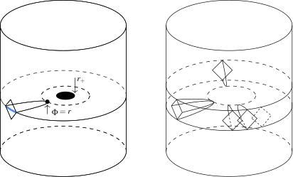
For a 3-dimensional metric that is separable and spherically symmetric,
| (102) |
one has and , so that the 3-dimensional Einstein-Hilbert action takes the form
| (103) |
A solution of the form (102) then directly gives rise to a solution of the 2-dimensional dilaton gravity action [38]
| (104) |
where the dilaton measures the radial coordinate in (102). For example, the BTZ solution
| (105) |
with horizon
| (106) |
given in terms of the radius of the conformal boundary of BTZ () and the inverse temperature , gives rise to the AdS2-black hole solution
| (107) |
with the same parameter . The dilaton in (103) will always appear in the dimensionless combination . It is then useful to introduce a dimensionless dilaton so that
| (108) |
defines a type of effective, running gravitational constant . In terms of the action (103) takes the JT form, and the AdS2-black hole solution above matches the notation in (142)-(143) (with ) if we define
| (109) | ||||
| (110) |
Here the arbitrary length scale was introduced to extract a dimensionless dilaton from (it is related to the arbitrary mass scale of [39] via ). Note also that matches the expression for the depth reached by a geodesic anchored to a BTZ boundary interval of length , as it should.
It follows directly from (108) that the dilaton
| (111) |
measures the area of the ‘hole’ of radius in the 3-dimensional background. It is argued in [40] that, while the area of a Ryu-Takayanagi surface in the locally AdS3 bulk is measured by one-interval entanglement of the dual CFT, the area of the hole in the bulk has to be measured as the envelope of a collection of Ryu-Takayanagi geodesics of fixed opening angle as illustrated in figure 5. It is then the quantity or ‘differential entropy’ that forms the CFT dual of the gravitational entropy of the hole,
| (112) |
and thus by the previous relation . This establishes equation (100). In particular, the relation in (100) between and the (effective) central charge of the dual CFT follows from the standard 3d/2d holographic dictionary entry [41]
| (113) |
and equation (109) for as a function of . The same relation appeared in [32] as a condition under which the Bekenstein-Hawking entropy of the JT solution takes the form of a Cardy formula. Indeed, this similarly follows from spherical dimensional reduction of the statement [42] that the Bekenstein-Hawking entropy of BTZ maps to the Cardy formula for the entropy of a thermal CFT2 counting the number of states with a given conformal dimension on the cylinder.
In the dual CFT, has the interpretation of ‘entanglement’ of the strip of width in the time direction, with caveats for referring to it as an actual entanglement discussed in [40, 43]. Let us remark here that equation (100) is then suggestive of the JT dilaton being holographically dual to the ‘entanglement’ of a time-like interval of length . It is unclear how to interpret such an object in the 1-dimensional dual theory. In this context it is perhaps important to stress that the one-interval entanglement in (100)-(101) is the one for a small interval compared to the size of the system. This means that for e.g. the BTZ background with conformal boundary the torus , it is given by
| (114) |
This is the correct expression for the entanglement in the high temperature limit or for small enough intervals. For intervals larger than a certain threshold known as the ‘entanglement shadow’, measures the length of winding geodesics in the bulk or ‘entwinement’ [44] in the dual CFT (rather than the length of the minimal geodesic in the bulk or entanglement in the dual CFT). The 1-dimensional theory dual to JT is obtained from the Liouville description of the 2-dimensional dual of asymptotically AdS3 in the limit [45, 46], where becomes pure entwinement.
Relevance to kinematic space
The interpretation of the vacuum contribution to the dilaton in (98) as the amount of entanglement removed as a result of a displacement of the boundary, is used in [6] to obtain an entropic derivation of the Schwarzian theory that describes the dynamics of the boundary in JT gravity. The argument makes use of entanglement renormalization, and is reminiscent of the concept of cMERA [47], short for continuous Multiscale Entanglement Renormalization Ansatz, with MERA a real-space renormalization group method in quantum many-body physics [48]. The description of kinematic space as a JT theory makes the relation between cMERA and the Schwarzian theory particularly natural, given the kinematic space/MERA proposal put forward in [1], which argues to consider MERA a discretization of kinematic space. It would be interesting to study the relation between cMERA and the Schwarzian theory further.
7 Discussion
We have discussed the JT dynamics of the kinematic space of 2-dimensional CFT’s with or without a boundary. The corresponding kinematic space respectively has an AdS or dS metric. The motivation for treating the ‘kinematic space identities’ in (24)-(27) and (43)-(46) as equations of motion initially was the mere observation that they coincided with the JT equations of motion. Doing so results in the concept of treating entanglement itself as a dynamic field. The goal of the paper is to provide an interpretation for the resulting JT theory, which turned out to be more straightforward in the case of boundary kinematic space, without claiming a complete analysis of the construction or a full understanding of its generality. In section 5 it was argued that the constructing principle (56) of boundary kinematic space can be interpreted as a 2-dimensional version of Jacobson’s maximal entanglement principle that couples the given bCFT to JT gravity on AdS. This discussion complements the results on the entanglement dynamics of a boundary CFT in [6] by providing a kinematic space point of view. It remains less clear however if a similar statement can be made for the de Sitter kinematic space discussed in section 3. What can be repeated for de Sitter, with the same conclusions, is the JT gravity discussion in section 6 leading to equation (94), with the remark that being a spacelike rather than a timelike Killing vector renders the ‘thermodynamic quantities’ of section 6.2 less physical meaning.
There is another context in which the coupling of a CFT to JT(-like) gravity appears, namely in the theory obtained by turning on a deformation of the CFT [49, 50, 51]. It would be interesting to study any connection of the theory to this work.
We would also like to understand better the relations between the different Liouville theories that appear in the AdS3/CFT2 context: the kinematic space Liouville theory of section 2 and the Liouville theory describing the asymptotic dynamics of AdS3, as well as the Liouville theory associated with complexity of [52]. Related questions are raised by the discussion of the interpretation of the JT dilaton from a dimensional reduction from AdS3 standpoint in section 6.4.
We leave these problems for future study.
Acknowledgements.
I am very grateful to Herman Verlinde for many insightful discussions and collaboration on a closely related paper. I further would like to thank Thomas Mertens in particular, for many helpful comments and discussions, as well as Steve Carlip, Bartek Czech, Ted Jacobson, Finn Larsen, Aitor Lewkowycz, Seth Lloyd, Mark Mezei, Charles Rabideau, Antony Speranza, Joaquin Turiaci, and Zhenbin Yang. This work is supported by the Research Foundation-Flanders (FWO Vlaanderen).Appendix A Jackiw-Teitelboim gravity
JT action and equations of motion
The Jackiw-Teitelboim theory [53, 54] is the dilaton gravity theory
| (115) |
with a linear potential
| (116) |
and a matter action that describes a field theory coupled to the metric . We assume that field theory to be conformal, and furthermore assume to be independent of the dilaton, such that variation with respect to the dilaton inforces the constant curvature equation
| (117) |
Variation with respect to the metric gives
| (118) |
with
| (119) | ||||
| (120) |
The equation of motion
| (121) |
can be split up in a traceless and a trace part
| (122) | ||||
| (123) |
For (classical) conformal matter, , and in ‘AdS’ conformal gauge (, ), the JT equations of motion (EOM) read
| (124) | ||||
| (125) | ||||
| (126) | ||||
| (127) |
If we change the sign of the potential to such that is imposed, then in ‘dS’ conformal gauge (, ), the JT EOM (124)-(127) are unchanged up to the sign of :
| (128) | ||||
| (129) | ||||
| (130) | ||||
| (131) |
Semi-classically, the trace anomaly is taken into account by considering the effective action , with the Polyakov action [55, 32]
| (132) |
with large. The semi-classical JT EOM then become (in AdS conformal gauge)
| (133) | ||||||
| (134) | ||||||
| (135) | ||||||
| (136) |
with covariant stress tensor components , and in particular so that, upon use of the Liouville equation , the last EOM reads
| (137) |
It follows that the solution is related to a solution of the classical EOM by (and replaced by ). Assuming the constant shift can be absorbed in the vacuum contribution , the vacuum-subtracted semi-classical dilaton obeys
| (138) | ||||
| (139) |
as if it were a classical dilaton , with the vacuum-subtracted, covariant stress tensor expectation value.
Solutions of JT
The general solution of the homogeneous JT EOM, (121) with , is given by an AdS2-black hole metric and a dilaton profile, which in Poincaré covering coordinates reads
| (140) | ||||
| (141) |
Here and are integration constants with dimension of length and one over length squared respectively, and we use the notation for the dilaton to indicate it is a vacuum solution. The geometry, illustrated in figure 4 (left), spans a triangular region with a boundary at . The quantity is related to the energy of the black hole solution and vanishes in the Poincaré solution.
The solution can alternatively be written in black hole coordinates or that cover the black hole triangle and are natural from a dimensional reduction viewpoint [38],
| (142) | ||||
| (143) |
In these coordinates, the Killing horizon of the solution is at or , where the dilaton takes the value
| (144) |
The transformation to the Poincaré covering coordinates is given by
| (145) |
The general solution of the inhomogeneous JT EOM (121) still has the same constant curvature metric. The dilaton however receives a stress tensor dependent contribution, which we will denote :
| (146) | ||||
| (147) |
To infer this form of the solution from its more general form in terms of integration functions in [55] and [32] requires two remarks. First, we have imposed reflective boundary conditions on the stress tensor
| (148) |
Second, any ambiguity in the choice of integration limit ( in the notation of [55]) can be absorbed in a redefinition of the integration constants in (we are thus free to choose in the notation of [55]).
Appendix B Iyer-Wald formalism
We recall the Iyer-Wald (IW) formalism, following the notation of [25]. Given a Lagrangian , one defines the energy variation through a region as
| (149) |
in terms of the symplectic current
| (150) |
where denotes the equations of motion for the dynamical fields and the symplectic potential (). is the current associated with the invariance of the Lagrangian under diffeomorphisms , and is conserved on-shell. The corresponding Noether charge is defined as
| (151) |
with the constraint equations, such that [56]. An IW first law is obtained when evaluating the relation
| (152) |
for a particular choice of diffeomorphism , usually a Killing vector ( for gravitational fields , so that the symplectic current, which is bilinear in the variations, vanishes).
Now let us apply the IW formalism to a gravitational theory with an action that depends on dynamic gravitational fields (including the metric) and matter fields , for a region and a vector that obeys . On a solution, , and as ,
| (153) |
Following the partition of the action in a gravitational and a matter part, the left hand side splits in a gravitational part and a matter part . The right hand side can be rewritten making use of (151) and assuming the variation is to a nearby solution (so that ), obtaining
| (154) |
This expresses that the on-shell vanishing of the linearized constraint equations is equivalent to the on-shell identity
| (155) |
References
- (1) B. Czech, L. Lamprou, S. McCandlish and J. Sully, Integral Geometry and Holography, JHEP 10 (2015) 175, [1505.05515].
- (2) J. de Boer, M. P. Heller, R. C. Myers and Y. Neiman, Holographic de Sitter Geometry from Entanglement in Conformal Field Theory, Phys. Rev. Lett. 116 (2016) 061602, [1509.00113].
- (3) B. Czech, L. Lamprou, S. McCandlish, B. Mosk and J. Sully, A Stereoscopic Look into the Bulk, JHEP 07 (2016) 129, [1604.03110].
- (4) J. de Boer, F. M. Haehl, M. P. Heller and R. C. Myers, Entanglement, holography and causal diamonds, JHEP 08 (2016) 162, [1606.03307].
- (5) B. Czech, L. Lamprou, S. McCandlish, B. Mosk and J. Sully, Equivalent Equations of Motion for Gravity and Entropy, JHEP 02 (2017) 004, [1608.06282].
- (6) N. Callebaut and H. Verlinde, Entanglement Dynamics in 2D CFT with Boundary: Entropic origin of JT gravity and Schwarzian QM, 1808.05583.
- (7) A. Karch, J. Sully, C. F. Uhlemann and D. G. E. Walker, Boundary Kinematic Space, JHEP 08 (2017) 039, [1703.02990].
- (8) T. Jacobson, Entanglement Equilibrium and the Einstein Equation, Phys. Rev. Lett. 116 (2016) 201101, [1505.04753].
- (9) C. Holzhey, F. Larsen and F. Wilczek, Geometric and renormalized entropy in conformal field theory, Nucl. Phys. B424 (1994) 443–467, [hep-th/9403108].
- (10) N. Seiberg, Notes on quantum Liouville theory and quantum gravity, Prog. Theor. Phys. Suppl. 102 (1990) 319–349.
- (11) A. C. Wall, Testing the Generalized Second Law in 1+1 dimensional Conformal Vacua: An Argument for the Causal Horizon, Phys. Rev. D85 (2012) 024015, [1105.3520].
- (12) S. de Haro, S. N. Solodukhin and K. Skenderis, Holographic reconstruction of space-time and renormalization in the AdS / CFT correspondence, Commun. Math. Phys. 217 (2001) 595–622, [hep-th/0002230].
- (13) M. M. Roberts, Time evolution of entanglement entropy from a pulse, JHEP 12 (2012) 027, [1204.1982].
- (14) O. Coussaert, M. Henneaux and P. van Driel, The Asymptotic dynamics of three-dimensional Einstein gravity with a negative cosmological constant, Class. Quant. Grav. 12 (1995) 2961–2966, [gr-qc/9506019].
- (15) K. Bautier, F. Englert, M. Rooman and P. Spindel, The Fefferman-Graham ambiguity and AdS black holes, Phys. Lett. B479 (2000) 291–298, [hep-th/0002156].
- (16) S. Carlip, Dynamics of asymptotic diffeomorphisms in (2+1)-dimensional gravity, Class. Quant. Grav. 22 (2005) 3055–3060, [gr-qc/0501033].
- (17) H. Casini, M. Huerta and R. C. Myers, Towards a derivation of holographic entanglement entropy, JHEP 05 (2011) 036, [1102.0440].
- (18) C. T. Asplund, N. Callebaut and C. Zukowski, Equivalence of Emergent de Sitter Spaces from Conformal Field Theory, JHEP 09 (2016) 154, [1604.02687].
- (19) J. Cardy and E. Tonni, Entanglement hamiltonians in two-dimensional conformal field theory, J. Stat. Mech. 1612 (2016) 123103, [1608.01283].
- (20) S. Lloyd, The quantum geometric limit, 1206.6559.
- (21) P. Bueno, V. S. Min, A. J. Speranza and M. R. Visser, Entanglement equilibrium for higher order gravity, Phys. Rev. D95 (2017) 046003, [1612.04374].
- (22) S. Gao and R. M. Wald, The ’Physical process’ version of the first law and the generalized second law for charged and rotating black holes, Phys. Rev. D64 (2001) 084020, [gr-qc/0106071].
- (23) M. Spradlin and A. Strominger, Vacuum states for AdS(2) black holes, JHEP 11 (1999) 021, [hep-th/9904143].
- (24) J. Maldacena, D. Stanford and Z. Yang, Conformal symmetry and its breaking in two dimensional Nearly Anti-de-Sitter space, PTEP 2016 (2016) 12C104, [1606.01857].
- (25) V. Iyer and R. M. Wald, Some properties of Noether charge and a proposal for dynamical black hole entropy, Phys. Rev. D50 (1994) 846–864, [gr-qc/9403028].
- (26) P. D. Hislop and R. Longo, Modular Structure of the Local Algebras Associated With the Free Massless Scalar Field Theory, Commun. Math. Phys. 84 (1982) 71.
- (27) C. R. Nappi and A. Pasquinucci, Thermodynamics of two-dimensional black holes, Mod. Phys. Lett. A7 (1992) 3337–3346, [gr-qc/9208002].
- (28) D. Grumiller and R. McNees, Thermodynamics of black holes in two (and higher) dimensions, JHEP 04 (2007) 074, [hep-th/0703230].
- (29) R. B. Mann and S. F. Ross, The D 2 limit of general relativity, Class. Quant. Grav. 10 (1993) 1405–1408, [gr-qc/9208004].
- (30) M. Cadoni, Conformal equivalence of 2-D dilaton gravity models, Phys. Lett. B395 (1997) 10–15, [hep-th/9610201].
- (31) D. Grumiller and R. Jackiw, Liouville gravity from Einstein gravity, in Recent developments in theoretical physics, S. Gosh, G. Kar, 2010. World Scientific, Singapore,2010, p.331, 2007. 0712.3775.
- (32) J. Engelsoy, T. G. Mertens and H. Verlinde, An investigation of AdS2 backreaction and holography, JHEP 07 (2016) 139, [1606.03438].
- (33) K. Jensen, Chaos in AdS2 Holography, Phys. Rev. Lett. 117 (2016) 111601, [1605.06098].
- (34) T. M. Fiola, J. Preskill, A. Strominger and S. P. Trivedi, Black hole thermodynamics and information loss in two-dimensions, Phys. Rev. D50 (1994) 3987–4014, [hep-th/9403137].
- (35) J. Gegenberg, G. Kunstatter and D. Louis-Martinez, Observables for two-dimensional black holes, Phys. Rev. D51 (1995) 1781–1786, [gr-qc/9408015].
- (36) R. B. Mann, Conservation laws and 2-D black holes in dilaton gravity, Phys. Rev. D47 (1993) 4438–4442, [hep-th/9206044].
- (37) M. D. McGuigan, C. R. Nappi and S. A. Yost, Charged black holes in two-dimensional string theory, Nucl. Phys. B375 (1992) 421–450, [hep-th/9111038].
- (38) A. Achucarro and M. E. Ortiz, Relating black holes in two-dimensions and three-dimensions, Phys. Rev. D48 (1993) 3600–3605, [hep-th/9304068].
- (39) D. Grumiller, W. Kummer and D. V. Vassilevich, Dilaton gravity in two-dimensions, Phys. Rept. 369 (2002) 327–430, [hep-th/0204253].
- (40) V. Balasubramanian, B. D. Chowdhury, B. Czech, J. de Boer and M. P. Heller, Bulk curves from boundary data in holography, Phys. Rev. D89 (2014) 086004, [1310.4204].
- (41) J. D. Brown and M. Henneaux, Central Charges in the Canonical Realization of Asymptotic Symmetries: An Example from Three-Dimensional Gravity, Commun. Math. Phys. 104 (1986) 207–226.
- (42) A. Strominger, Black hole entropy from near horizon microstates, JHEP 02 (1998) 009, [hep-th/9712251].
- (43) B. Czech, P. Hayden, N. Lashkari and B. Swingle, The Information Theoretic Interpretation of the Length of a Curve, JHEP 06 (2015) 157, [1410.1540].
- (44) V. Balasubramanian, B. D. Chowdhury, B. Czech and J. de Boer, Entwinement and the emergence of spacetime, JHEP 01 (2015) 048, [1406.5859].
- (45) T. G. Mertens, G. J. Turiaci and H. L. Verlinde, Solving the Schwarzian via the Conformal Bootstrap, JHEP 08 (2017) 136, [1705.08408].
- (46) T. G. Mertens, The Schwarzian Theory - Origins, JHEP 05 (2018) 036, [1801.09605].
- (47) J. Haegeman, T. J. Osborne, H. Verschelde and F. Verstraete, Entanglement Renormalization for Quantum Fields in Real Space, Phys. Rev. Lett. 110 (2013) 100402, [1102.5524].
- (48) G. Vidal, Entanglement Renormalization, Phys. Rev. Lett. 99 (2007) 220405, [cond-mat/0512165].
- (49) F. A. Smirnov and A. B. Zamolodchikov, On space of integrable quantum field theories, Nucl. Phys. B915 (2017) 363–383, [1608.05499].
- (50) S. Dubovsky, V. Gorbenko and M. Mirbabayi, Asymptotic fragility, near AdS2 holography and , JHEP 09 (2017) 136, [1706.06604].
- (51) S. Dubovsky, V. Gorbenko and G. Hernández-Chifflet, partition function from topological gravity, JHEP 09 (2018) 158, [1805.07386].
- (52) P. Caputa, N. Kundu, M. Miyaji, T. Takayanagi and K. Watanabe, Liouville Action as Path-Integral Complexity: From Continuous Tensor Networks to AdS/CFT, JHEP 11 (2017) 097, [1706.07056].
- (53) R. Jackiw, Lower Dimensional Gravity, Nucl. Phys. B252 (1985) 343–356.
- (54) C. Teitelboim, Gravitation and Hamiltonian Structure in Two Space-Time Dimensions, Phys. Lett. 126B (1983) 41–45.
- (55) A. Almheiri and J. Polchinski, Models of AdS2 backreaction and holography, JHEP 11 (2015) 014, [1402.6334].
- (56) V. Iyer, Lagrangian perfect fluids and black hole mechanics, Phys. Rev. D55 (1997) 3411–3426, [gr-qc/9610025].