Phase ordering kinetics of the long-range Ising model
Abstract
We use an efficient method that eases the daunting task of simulating dynamics in spin systems with long-range interaction. Our Monte Carlo simulations of the long-range Ising model for the nonequilibrium phase ordering dynamics in two spatial dimensions perform significantly faster than the standard Metropolis approach and considerably more efficiently than the kinetic Monte Carlo method. Importantly, this enables us to establish agreement with the theoretical prediction for the time dependence of domain growth, in contrast to previous numerical studies. This method can easily be generalized to applications in other systems.
Generic models of statistical physics exhibiting a transition from disordered to ordered states have been proved to be instrumental for understanding the dynamics in diverse fields, from species evolution [1] to traffic flow [1], from economic dynamics [2] to rainfall dynamics [3]. An extensively used paradigm is the Ising model with nearest-neighbor (NNIM) interaction [4, 5]. Even the complex neural dynamics of brain depends on similar underlying mechanisms [6]. The maximum entropy models obtained from experimental data upon mapping the spiking activities of the neurons onto spin variables are equivalent to Ising models [7]. However, it is believed that the neuron activities are effectively modelled by long-distance communications [6]. In nature, also many other intermolecular interactions are evidently long-range, e.g., electrostatic forces, polarization forces, etc. Hence, a more complete picture calls for employing models that consider long-range interactions.
The simplest generic model system is the long-range Ising model (LRIM), which on a -dimensional lattice is described by the Hamiltonian
| (1) |
where spins , is the distance between the spins at site and , and is the interaction strength. The model exhibits a para- to ferro-magnetic phase transition. Naturally, simulations of such systems with long-range interaction are computationally far more expensive than its short-range counterpart. For equilibrium studies, the advent of various collective updates based on the Swendsen-Wang cluster algorithm [8] allows one to perform efficient Monte Carlo (MC) simulations [9, 10, 11]. Conversely, for understanding the nonequilibrium ordering kinetics following a quench from the high-temperature disordered phase into the ordered phase below the critical temperature , one is restricted to use only local moves, viz., single spin flips. This makes MC simulations of ordering kinetics in LRIM severely expensive even with present-day computational facilities, and therefore, they have rarely been attempted [12].
The understanding of ferromagnetic ordering kinetics in NNIM is well developed [4, 5]. It is characterized by formation and growth of domains of like spins and is a scaling phenomenon, i.e., the characteristic length scale a.k.a. the domain size at time follows the Lifshitz-Cahn-Allen (LCA) law [4]: which can be derived by considering that grows via reduction of the curvature of the domain walls. Similarly for the LRIM the growth is likely to be driven by interactions between domain walls. Assuming this growth as a scaling phenomenon and using an “energy scaling” argument it has been predicted that [13, 14, 15]
| (2) |
i.e., (i) in the “truly” long-range regime for , the growth exponent is dependent, (ii) at the crossover point , the growth follows the LCA law with a multiplicative logarithmic correction, and (iii) for , LRIM behaves asymptotically as the NNIM with . There exist few attempts to confirm these predictions via numerical solution of Ginzburg-Landau-type [16] or Langevin-type [17, 18] dynamical equations. The only available results from MC simulations [12] in this regard tackles the expensive calculation of the local energy involving all the spins by using a cut-off distance for in (1). Importantly, in disagreement with (2), is found there to be no different than in NNIM for all , thus suggesting a universal nonequilibrium behavior. In equilibrium it is well established both theoretically [19, 20, 21] and in simulations [22, 23, 24] that critical exponents are not universal. For example, in the LRIM, for the critical exponent takes its mean-field value, followed by an intermediate range where it is -dependent, and for it behaves like in the NNIM. The value of the crossover point is still disputed [24] and predicted to be [20] or [21]. In this Letter, we present results from MC simulations for the ordering kinetics of LRIM in using our efficient approach with the aim to check the -dependence of the growth exponent .
In a standard Metropolis simulation [25] for kinetics of LRIM one attempts to flip a randomly chosen spin with probability , where is the Boltzmann constant, is the temperature and is the change in energy due to the flip. The aim of our approach is to avoid the expensive calculation of at every attempt. Instead we store the effective field, assigned to each spin, and only update other spin flips to this effective field 11 1 We thank A. Hucht for informing us after completion of this work, that such an approach has already been very briefly mentioned in Ref. [42] where the method was used to simulate the Heisenberg model with dipolar interactions..
| Clocks () |
|---|
When simulating a long-range interacting system using periodic boundary conditions (via minimum-image convention), one encounters strong finite-size effects. We circumvent this problem by using Ewald summation [27, 24, 11] for calculating the effective interaction . To prepare an initial configuration that mimics a high-temperature paramagnetic phase () we choose a square lattice having linear dimension with randomly up and down spins. Next, for each spin , we store the effective field
| (3) |
The Metropolis simulation at any given temperature can now be done efficiently with the advantage of having these stored , in the following way. Using Eq. (3) one can write down the change in energy due to an attempted flip of a randomly chosen spin as
| (4) |
Now if the spin is flipped the effective field of any other spin accounts for a change of , thus . This operation can be performed with roughly the same computational effort as calculating a single in the traditional approach. However, one does this only for accepted spin flips. Thus many spin-flip attempts can be made without this update of , facilitating a significant speedup.
The above approach is reminiscent of the -fold way or kinetic MC (KMC) simulations [28, 29], which have been extensively used for short-range models. In KMC for the NNIM the major advantage lies in categorizing the local spin environment into classes. To the best of our knowledge, KMC has never been applied in the LRIM, presumably because construction of classes is impossible in the long-range case and the probability of every spin flip needs to be calculated at each step. Combining the idea of updating the effective fields or the probabilities during KMC, of course, improves the performance, but even then, our approach provides times better performance 22 2 In our approach the average waiting time between spin-flips is , as it can be shown that for the coarsening period the average acceptance . Thus we have to calculate involving the computationally expensive exponential function, only times, whereas in KMC, the exponential function has to be calculated times always. at quench temperature 33 3 The value of for the LRIM is extracted by a power-law fit of form to the data presented in Ref. [24]. For the purpose of nonequilibrium simulations the precise value of is not important and this rather crude estimate is sufficient., which will be used subsequently for all our simulations. For this and all following analyses, the unit of time is one MC step (MCS) that consists of spin-flip attempts. The results for the ordering kinetics are averaged over independent realizations for and realizations for .

In Table 1 we tabulated the number of CPU clocks needed for our method to perform MCS for different . Roughly the clock time for all the is . To run the same number of MCS using the standard approach the clock time is . Thus an improvement factor can be achieved with this algorithm for the LRIM at the chosen quench temperature. Since for our method the lower the acceptance rate the more one gains in speed, at lower temperatures the efficiency gain with respect to the standard approach becomes higher, whereas at both of them should have identical run time. Note that our algorithm becomes faster as the simulation moves on because of the lower acceptance rates when the system approaches the ordered phase, and we emphasize it does not use any cut-off in .
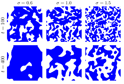
Having the new methodology in place, we move on to explore the kinetics of the ferromagnetic ordering in LRIM. In Fig. 1 we present evolution snapshots for three different values of from a typical quench. Apparently the structural changes during the evolution are no different than in NNIM [4]. From the snapshots at the same time for different it is evident that the smaller the value of the faster is the growth. However, one needs to estimate the growth exponents in order to overrule the claim of the scaling equivalence for different reported in Ref. [12].


We now check the scaling of the morphology-characterizing two-point equal-time correlation function and its Fourier transform, the structure factor . Figure 2(a) presents at different times for , showing the signature of a growing length scale with time. The multiplicative scaling during the growth is confirmed by the data collapse as shown in Fig. 2(b), on plotting the against where the length scale is extracted from the criterion . The data at large for the latest time seems to show some discrepancy attributed to finite-size effects. However, the scaling of the structure factor that forms a basic assumption when deriving the theoretical growth laws for LRIM [14, 15], is confirmed convincingly as shown in Fig. 2(c). Similar respective behavior is observed when scaled and at the same time are plotted for different in Fig. 3. The slower decay of for smaller values of could be an indication of the inverse relation of the growth exponent with , as predicted in Eq. (2). Contrasting, the scaled for different in Fig. 3(b) show reasonably good overlap. The solid lines in Fig. 2(c) and Fig. 3(b) depict the consistency of the data with the Porod tail [32]: at large wave number .
The multiplicative scaling of the morphology-characterizing functions indeed suggests the presence of scaling of the growing length scale. Hence, shifting our focus on the growth exponent in Fig. 4(a) we present the time dependence of the length scale for . The behavior is certainly not (shown by the dashed line), but in fact the data for all follow the predicted behavior of until they show deviations due to finite-size effects. This already indicates that the underlying scaling behavior is indeed consistent with (2). Nevertheless, to further strengthen the claim and to gauge the effect of a finite system size we call for a finite-size scaling (FSS) analysis [33, 34] which recently has been successfully employed in kinetics of other systems [35, 36, 37]. Quantifying the growth including an initial crossover time and length one can write down the ansatz and construct a FSS function with the scaling variable . In the scaling regime one expects . Thus on plotting as a function of for different one must observe a data collapse with behavior for large provided is chosen appropriately. We did this exercise for different choosing from (2). However, not all of them are presented here, but rather a representative plot for is shown in the inset of Fig. 4(a). The collapsed data is consistent with the underlying master curve . Considering the collapsed data for all and fitting the ansatz by treating () as a fit parameter, we obtain with reasonable reduced chi-squared within the range . Similarly, if we fix according to (2) and use the same fit range as above we again get a reasonable .
In Fig. 4(b) we present the time dependence of the length scale for different . Our data clearly indicates that becomes larger as decreases. Importantly in each case the data follows the theoretically predicted behavior (2) shown as solid lines, in contradiction with results [12] reporting independent of . At the crossover point our data follows the LCA growth with multiplicative logarithmic correction: , albeit a power-law growth with cannot unprejudiced be ruled out. However, in accordance with (2) for in the post-crossover regime () the growth appears to be , as expected for the NNIM. To consolidate the visual validation we also performed for each case least-square fits of prediction (2) and verified the predicted exponent values [38]. In the inset of Fig. 4(b) we show a plot of the length scale obtained from simulations using different cut-off radii in Eq. (1) for . For the largest the data follows behavior as is observed without any cut-off, whereas the cases with smaller obey the LCA law. Thus, in conjunction with the previously reported simulation [12] one can infer that the use of a relatively small make the spins interact only on short range leading to -independent growth exponents.
To conclude, we have studied the kinetics of ferromagnetic ordering using the long-range Ising model in spatial dimensions via MC simulations using an efficient method. We have introduced the idea of storing the effective field for each spin that helps to reduce the expensive calculation of local energy changes involving all the spins at every step. Our approach speeds up the simulation by a factor of compared to the standard Metropolis algorithm, and is even considerably faster than the efficient kinetic MC method. This enables us to simulate systems as big as spins without using any cut-off radius in the distance-dependent power-law interaction. Results obtained from our simulations are the first confirmation of the theoretical prediction in (2) for the growth laws in the long-range Ising model [14, 13, 15]. We have also demonstrated that the inappropriate use of a cut-off radius in the local-energy calculation may lead to a different growth exponent, explaining the mismatch between previous simulation results [12] and theory.
In equilibrium, the long-range Ising model has a dimension-dependent crossover behavior of the critical exponents [19, 20, 21, 22, 23, 24], while in nonequilibrium the prediction (2) is expected to be independent of the dimension. In this light, we take the ordering kinetics of the case as our next endeavor to check this dimension independence 44 4 Work in progress. Our method shall trigger interests to explore other aspects associated with ordering phenomena in the long-range Ising model, viz., aging and related dynamical scaling [40]. The generic simple feature of the method shall ensure its facile adoptions to nonequilibrium simulations of other models, viz., -state Potts and clock models. In view of the delicate cut-off dependence, it would also be interesting to revisit the ordering phenomenon in long-range liquid crystals [41]. Although originally designed for simulating dynamics, our method should be proven to be handy for equilibrium simulations of systems with long-range interactions, for which there (currently) exist no cluster algorithms, e.g., (lattice-) polymers [31].
Acknowledgements.
This project was funded by the Deutsche Forschungsgemeinschaft (DFG) under Grant Nos. JA 483/33-1 and SFB/TRR 102 (project B04), and further supported by the Leipzig Graduate School of Natural Sciences “BuildMoNa”, the Deutsch-Französische Hochschule (DFH-UFA) through the Doctoral College “” under Grant No. CDFA-02-07, and the EU Marie Curie IRSES network DIONICOS under Grant No. PIRSES-GA-2013-612707. We thank Stefan Schnabel for a very important suggestion.References
- [1] P. Bak, How Nature Works (Oxford University Press, Oxford, 1997).
- [2] T. Lux and M. Marchesi, “Scaling and criticality in a stochastic multi-agent model of a financial market,” Nature 397, 498 (1999).
- [3] O. Petrs and D. Neelin, “Critical phenomena in atmospheric precipitation,” Nat. Phys. 2, 393 (2006).
- [4] A.J. Bray, “Theory of phase-ordering kinetics,” Adv. Phys. 51, 481 (2002).
- [5] S. Puri and V. Wadhawan, eds., Kinetics of Phase Transitions (CRC Press, Boca Raton, 2009).
- [6] J.M. Beggs and D. Plenz, “Neuronal avalanches in neocortical circuits,” J. Neurosci. 24, 11167 (2003).
- [7] E. Schneidman, M.J. Berry, R. Segev, and W. Bialek, “Weak pairwise correlations imply strongly correlated network states in a neural population,” Nature 440, 1007 (2006).
- [8] R.H. Swendsen and J.S. Wang, “Nonuniversal critical dynamics in Monte Carlo simulations,” Phys. Rev. Lett. 58, 86 (1987).
- [9] E. Luijten and H.W.J. Blöte, “Monte Carlo method for spin models with long-range interactions,” Int. J. Mod. Phys. C 6, 359 (1995).
- [10] K. Fukui and S. Todo, “Order- cluster Monte Carlo method for spin systems with long-range interactions,” J. Comput. Phys. 228, 2629 (2009).
- [11] E. Flores-Sola, M. Weigel, R. Kenna, and B. Berche, “Cluster Monte Carlo and dynamical scaling for long-range interactions,” Eur. Phys. J. Spec. Top. 226, 581 (2017).
- [12] J. Gundh, A. Singh, and R.K.B. Singh, “Ordering dynamics in neuron activity pattern model: An insight to brain functionality,” PloS one 10, e0141463 (2015).
- [13] A. J. Bray, “Domain-growth scaling in systems with long-range interactions,” Phys. Rev. E 47, 3191 (1993).
- [14] A.J. Bray and A.D. Rutenberg, “Growth laws for phase ordering,” Phys. Rev. E 49, R27 (1994).
- [15] A.D. Rutenberg and A.J. Bray, “Phase-ordering kinetics of one-dimensional nonconserved scalar systems,” Phys. Rev. E 50, 1900 (1994).
- [16] H. Hayakawa, T. Ishihara, K. Kawanishi, and T.S. Kobayakawa, “Phase-ordering kinetics in nonconserved scalar systems with long-range interactions,” Phys. Rev. E 48, 4257 (1993).
- [17] B.P. Lee and J.L. Cardy, “Phase ordering in one-dimensional systems with long-range interactions,” Phys. Rev. E 48, 2452 (1993).
- [18] I. Ispolatov, “Persistence in systems with algebraic interaction,” Phys. Rev. E 60, R2437 (1999).
- [19] G. Stell, “Extension of the Ornstein-Zernike theory of the critical region. II,” Phys. Rev. B 1, 2265 (1970).
- [20] M.E. Fisher, S. Ma, and B.G. Nickel, “Critical exponents for long-range interactions,” Phys. Rev. Lett. 29, 917 (1972).
- [21] J. Sak, “Recursion relations and fixed points for ferromagnets with long-range interactions,” Phys. Rev. B 8, 281 (1973).
- [22] E. Luijten and H.W.J. Blöte, “Classical critical behavior of spin models with long-range interactions,” Phys. Rev. B 56, 8945 (1997).
- [23] E. Luijten and H.W.J. Blöte, “Boundary between long-range and short-range critical behavior in systems with algebraic interactions,” Phys. Rev. Lett. 89, 025703 (2002).
- [24] T. Horita, H. Suwa, and S. Todo, “Upper and lower critical decay exponents of Ising ferromagnets with long-range interaction,” Phys. Rev. E 95, 012143 (2017).
- [25] D.P. Landau and K. Binder, A Guide to Monte Carlo Simulations in Statistical Physics (Cambridge University Press, Cambridge, 2014).
- [26] We thank A. Hucht for informing us after completion of this work, that such an approach has already been very briefly mentioned in Ref. [42] where the method was used to simulate the Heisenberg model with dipolar interactions.
- [27] P. Ewald, “Die Berechnung optischer und elektrostatischer Gitterpotentiale,” Ann. Phys. 369, 253 (1921).
- [28] A.B. Bortz, M.H. Kalos, and J.L. Lebowitz, “A new algorithm for Monte Carlo simulation of Ising spin systems,” J. Comput. Phys. 17, 10 (1975).
- [29] A. F. Voter, “Introduction to the kinetic Monte Carlo method,” in Radiation Effects in Solids, edited by K. E. Sickafus, E. A. Kotomin, and B. P. Uberuaga (Springer, Dordrecht, 2007) p. 1.
- [30] In our approach the average waiting time between spin-flips is , as it can be shown that for the coarsening period the average acceptance . Thus we have to calculate involving the computationally expensive exponential function only times, whereas in KMC, the exponential function has to be calculated times always.
- [31] The value of for the LRIM is extracted by a power-law fit of form to the data presented in Ref. [24]. For the purpose of nonequilibrium simulations the precise value of is not important and this rather crude estimate is sufficient.
- [32] G. Porod, “General theory,” in Small Angle X-ray Scattering, edited by O. Glatter and O. Kratky (Academic Press, London, 1982) p. 17.
- [33] S. Majumder and S.K. Das, “Domain coarsening in two dimensions: Conserved dynamics and finite-size scaling,” Phys. Rev. E 81, 050102 (2010).
- [34] S.K. Das, S. Roy, S. Majumder, and S. Ahmad, “Finite-size effects in dynamics: Critical vs. coarsening phenomena,” Europhys. Lett. 97, 66006 (2012).
- [35] S. Majumder and W. Janke, “Cluster coarsening during polymer collapse: Finite-size scaling analysis,” Europhys. Lett. 110, 58001 (2015).
- [36] S. Majumder, J. Zierenberg, and W. Janke, “Kinetics of polymer collapse: Effect of temperature on cluster growth and aging,” Soft Matter 13, 1276 (2017).
- [37] H. Christiansen, S. Majumder, and W. Janke, “Coarsening and aging of lattice polymers: Influence of bond fluctuations,” J. Chem. Phys. 147, 094902 (2017).
- [38] W. Janke, H. Christiansen, and S. Majumder, “Coarsening in the long-range Ising model: Metropolis versus Glauber criterion,” to appear in J. Phys.: Conf. Ser. (2019).
- [39] Work in progress.
- [40] M. Henkel and M. Pleimling, Non-Equilibrium Phase Transitions, Vol. 2: Ageing and Dynamical Scaling far from Equilibrium (Springer, Heidelberg, 2010).
- [41] A. Singh, S. Ahmad, S. Puri, and S. Singh, “Ordering kinetics in liquid crystals with long-ranged interactions,” Eur. Phys. J. E 37, 2 (2014).
- [42] A. Hucht, A. Moschel, and K.D. Usadel, “Monte-Carlo study of the reorientation transition in Heisenberg models with dipole interactions,” J. Magn. Magn. Mater 148, 32 (1995).