Centroid estimation based on symmetric KL divergence for Multinomial text classification problem
Abstract
We define a new method to estimate centroid for text classification based on the symmetric KL-divergence between the distribution of words in training documents and their class centroids. Experiments on several standard data sets indicate that the new method achieves substantial improvements over the traditional classifiers.
Index Terms:
centroid estimation, KL divergence, text classification, naive bayesI Introduction
Text classification problem has long been an interesting research field, the aim of text classification is to develop algorithm to find the categories of given documents. Text classification has many applications in natural language processing (NLP), such as spam filtering, email routing, and sentimental analysis. Despite intensive work,remains an open problem today.
This problem has been studied for many aspects, including: supervised classification problem, if we are given the labeled training data; unsupervised clustering problem, if we only have documents without labeling; as well as feature selection.
For supervised problem, if we assume that all the categories are independent multinomial distributions, and each document is a sample generated by that distribution, a straight forward idea is to using some linear models to distinguish them, such as support vector machine (SVM)[3, 6], which is used to find the ”maximum-margin hyperplane” that divides the documents with different labels. The algorithm is defined so that the distance between the hyperplane and the nearest sample from either group is maximized. The hyperplane can be written as the set of documents vector satisfying:
where is the normal vector to the hyperplane. Under the same assumption, another effective classifier, using scores based on the probability of given documents conditioned on the categories, is called naive Bayesian classifier[4, 7]. This classifier learns from training data to estimate the distribution of each categories, then we can compute the conditional probability of each documents given the class label by applying Bayes rule, then the predicting of the classes is done by choosing the highest posterior probability. The algorithm to get the label for a given document is given by:
When we understand the documents as sequence of words, to understand the order of the words, given the data set large enough, we can using deep learning models such as Recurrent Neural Network (RNN)[12, 8].
For unsupervised problem. We have traditional method SVD (Singular Value Decomposition)[1] for the dimension reduction and clustering. There also exist some algorithms based on EM algorithm, such as pLSA (Probabilistic latent semantic analysis)[5], which consider the probability of each co-occurrence as a mixture of conditionally independent multinomial distributions:
where and are observed words and documents, and been the words’ topic. As we mentioned, the parameters are learned by EM algorithm. Using the same idea, but assuming that the topic distribution has sparse Dirichlet prior, we have algorithm LDA (Latent Dirichlet allocation)[2]. The sparse Dirichlet priors encode the intuition that documents cover only a small set of topics and that topics use only a small set of words frequently. In practice, this results in a better disambiguation of words and a more precise assignment of documents to topics.
There are also many results in feature engineering, such as tf-idf[10], n-gram, or inproved tf-idf with other feature selection[11].
In this paper, we still assume that documents are generated according to a multinomial event model[9]. We defined a new method to estimate centroid based on the symmetric KL-divergence between the distribution of documents and their class centroids, which works better than original average estimated centroid in naive Bayes method.
Notations: In this paper, document belong to class with index is represented as a vector of word counts where is the vocabulary, and each indicates how often occurs in . denotes the centroid of the class , since we use the assumption that documents are generated according to a multinomial event model, satisfies:
II Our model
Let , be two multinomial distributions, the KL-divergence is defined as:
KL-divergence measures how much one probability distribution is different from another, it is strongly connected with naive bayes classifier. Given class prior probabilities and assuming independence of the words, normalize of document vector of , the most likely class for a document satisfying is computed as:
| (II.1) | |||||
To make it symmetric of and , we add in another term related to as regularizer to get symmetric KL-divergence:
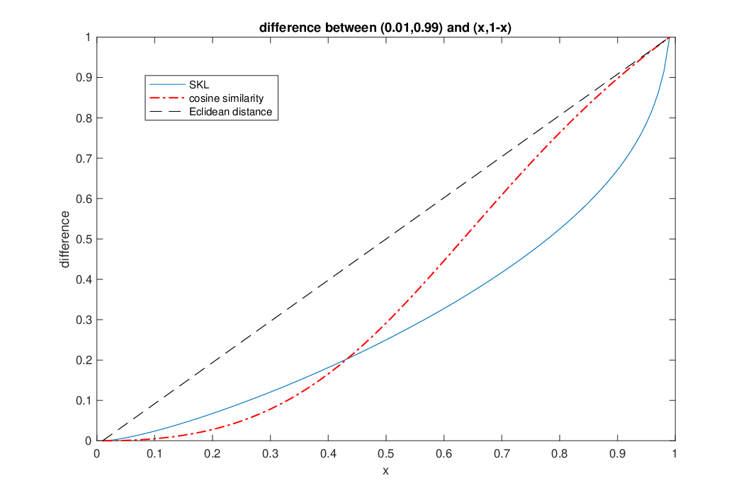
To compare several measures of difference of two distributions, let , , Figure.1 shows how the difference of two vectors change under different measures. We can see that for and far from each other, the difference of SKL decay faster, and for closer distributions, it decreases slower than linear speed. So SKL should be a good choice to distinguish distributions.
In the labeled training set, for each classes, we use SKL to find the centroid, whose sum of symmetric KL-divergence to all documents in that class reaches minimum, more specifically, the centoid is defined as following:
| (II.2) |
Let , since:
Take partial derivative to we obtain:
Thus:
III Minimization problem
To solve II.2 on the discrete probability manifold, the Wasserstein is used to get the gradient system. To this ends, suppose the graph structure is given where are nodes set containing all the words involved and defines the edge set which links the graph to be a connected graph. And in the examples below, the simplest histogram structure is used, that is, all the words are linked one by one in some order in a line. Also denote be the number of nodes on the graph.
Now consider a energy function , let
define the orientation on to be that for , the direction is from to if and that is arbitrary if , denoting as . Then the construction of the gradient of a potential function based on the orientation is
Then, an inner product can be written as
where
and the gradient flow under this metric is known as discrete 2-Wasserstein gradient flow since the discrete 2-Wasserstein distance is defined as
Now consider the energy function to be
and the gradient flow can be written as
Solving this ODE obtains the solution for problem II.2.
IV Experiment
We applied our method on seven topics of single labeled documents in Reuters-21578, we find the accuracy of naive bayes using our centroid estimator increasing faster than original method, see Figure.2, and when training size is large enough, our method achieves substantial improvements over the traditional method.

For each single class, the behave of our method versus traditional naive bayes estimator can be find in Figure.3. We can a clear increasing trend for topics as training size becoming larger.
| coffee | sugar | trade | ship | crude | interst | money-fx |
| 9.0348 | 8.9305 | 6.2703 | 9.1293 | 7.3662 | 7.4778 | 6.9361 |
Table.I shows the average SKL to other classes, from Figure.3 we can see that class ’trade’ is the only one doesn’t have trend of increasing, that might because it is very closed to other classes, and SKL cannot distinguish it well based on our observation in Figure1.

V Open problems
- •
We find better estimator for centroid using naive bayes, can we find similar result for other estimators?
- •
Can this centroid estimator be extended to be used in unsupervised learning problem?
- •
When we solve the minimization problem, we have a graph structure for each feature. We are using a connecting graph now, can we use the partially connected graph to demonstrate correlation of words?
References
- [1] Russ Albright. Taming text with the svd. SAS Institute Inc, 2004.
- [2] David M Blei, Andrew Y Ng, and Michael I Jordan. Latent dirichlet allocation. Journal of machine Learning research, 3(Jan):993–1022, 2003.
- [3] Corinna Cortes and Vladimir Vapnik. Support-vector networks. Machine learning, 20(3):273–297, 1995.
- [4] Nir Friedman, Dan Geiger, and Moises Goldszmidt. Bayesian network classifiers. Machine learning, 29(2-3):131–163, 1997.
- [5] Thomas Hofmann. Probabilistic latent semantic analysis. In Proceedings of the Fifteenth conference on Uncertainty in artificial intelligence, pages 289–296. Morgan Kaufmann Publishers Inc., 1999.
- [6] Thorsten Joachims. Text categorization with support vector machines: Learning with many relevant features. In European conference on machine learning, pages 137–142. Springer, 1998.
- [7] Pat Langley, Wayne Iba, Kevin Thompson, et al. An analysis of bayesian classifiers. In Aaai, volume 90, pages 223–228, 1992.
- [8] Pengfei Liu, Xipeng Qiu, and Xuanjing Huang. Recurrent neural network for text classification with multi-task learning. arXiv preprint arXiv:1605.05101, 2016.
- [9] Andrew McCallum, Kamal Nigam, et al. A comparison of event models for naive bayes text classification. In AAAI-98 workshop on learning for text categorization, volume 752, pages 41–48. Citeseer, 1998.
- [10] Juan Ramos et al. Using tf-idf to determine word relevance in document queries. In Proceedings of the first instructional conference on machine learning, volume 242, pages 133–142, 2003.
- [11] Karl-Michael Schneider. A new feature selection score for multinomial naive bayes text classification based on kl-divergence. In Proceedings of the ACL 2004 on Interactive poster and demonstration sessions, page 24. Association for Computational Linguistics, 2004.
- [12] Duyu Tang, Bing Qin, and Ting Liu. Document modeling with gated recurrent neural network for sentiment classification. In Proceedings of the 2015 conference on empirical methods in natural language processing, pages 1422–1432, 2015.