LYCEN 2018-08
Vacuum misalignment and pattern of scalar masses in the SU(5)/SO(5) composite Higgs model
Abstract
Composite Higgs models based on are characterised by the presence of custodial triplets, like the Georgi-Machacek model. We classify all the operators giving rise to the top mass and Higgs potential in presence of fermion partial compositeness, with top partners in two-index representations of . A detailed study of each operator allows us to find correlations in the couplings of Higgs and non-Higgs pseudo-Nambu-Goldstone bosons, which depend only on one, two or three independent parameters. We also analyse the Higgs potential, finding that a misalignment along the custodial invariant triplet direction is forbidden by CP conservation. Avoiding custodial breaking allows us to select a handful of feasible models, which feature universal patterns in the scalar masses related to their transformation properties under the custodial symmetry. Finally, we briefly study the LHC phenomenology of the scalars, which are always below 1 TeV even for multi-TeV condensation scales, and find promising same-sign lepton final states enriched by hard photons.
1 Introduction
The discovery of a scalar particle with properties compatible with those of the Standard Model (SM) Higgs boson – announced by the ATLAS [1] and CMS [2] collaborations in 2012 – has crowned with success the efforts made by a large community of physicists during more than forty years. Although the SM explains with extremely high precision almost all the data collected at particle colliders, there are still many aspects that are poorly understood or that cannot find an explanation within the current established framework. Leaving aside issues related to Naturalness and the Hierarchy problem, we mention that the SM does not provide any dynamical explanation to the mechanism of electroweak symmetry breaking (EWSB), the latter being a feature that plays a major role in the theory of interactions between fundamental particles. Since a large part of the theoretical issues in the SM, including triviality and stability [3, 4], are related to the scalar sector, all such problems do not affect theories in which the scalar states are of composite nature. Of course, complying with the experimental data requires to account for the existence of a scalar mode compatible with the discovered Higgs boson.
The Composite Higgs (CH) scenario represents a suitable framework for introducing a non-elementary scalar sector in the SM. We will consider the class of CH models in which the Higgs arises as a pseudo-Nambu-Goldstone boson (pNGB) of some spontaneously broken symmetry [5], related to a new confining sector. In particular, in CH models that admit an underlying fermionic theory, which we will denote as ‘realistic models’, the symmetry is assumed to be broken by the formation of a bilinear condensate of the new “hyperfermions” (HF) , interacting via a “hypercolour” (HC) dynamics that is responsible for the confinement. The underlying theories are selected in order to have a vacuum of the HC dynamics that does not break the SM gauge symmetry. Its alignment, leading to the EWSB, is then determined by the low-energy dynamics [5]. Remarkably, in realistic models, the Higgs is always accompanied by at least one additional pNGB [6], implying that the potential of the scalar sector is richer than the minimal one used in the SM. For instance, it can exhibit mass mixing among the different pNGBs, depending on their quantum numbers and on the alignment direction of the vacuum. In fact, the vacuum is usually assumed to be misaligned only along the Higgs direction, even though this is not the most general scenario. In this case, the relation between the vacuum misalignment angle [7] and the condensate scale is simply given by , where is the electroweak vacuum expectation value (VEV) in the SM. Furthermore, the Higgs does not mix with other pNGBs and its couplings are modified in a universal way (see, for instance, examples in Refs [8, 9]). 11 1 Mixing of the Higgs to other light scalars can be induced by adding ad-hoc couplings, like in Refs [10, 11], or by misaligning the vacuum in non-minimal ways, as shown in Ref. [9]. A mixing to a light composite spin-0 resonance, if present, is also inevitable [12]. However, especially in models where many neutral pNGBs are present, a more general vacuum structure cannot be excluded a priori neither by electroweak precision data, specifically the bounds on the parameter, nor by the measurement of Higgs couplings. In fact, the vacuum misalignment is not arbitrary, but fully determined by the couplings of the SM fields to the strong dynamics, and non-minimal alignments are in some cases unavoidable (see Ref. [9]).
All the features mentioned above are present in the CH model [7, 13, 14] that we consider in this work. The pNGBs can be conveniently classified on the (non-physical) vacuum that preserves the electroweak (EW) symmetry: in addition to a composite Higgs doublet, the other fields include a gauge singlet pseudo-scalar and three triplets, of hypercharge and . The low energy field content, therefore, resembles that of the Georgi-Machacek model [15, 16], with the addition of a singlet [17]. 22 2 In the composite case, however, the singlet cannot be Dark Matter, as it decays via topological anomalies [7]. The physical eigenstates, however, due to the mixing, do not correspond to the gauge ones. In fact, a simpler way to describe the mass spectrum is to use the custodial eigenstates [7], where the three triplets combine into a five-plet, a triplet and a singlet. This approach is quite useful because the diagonal custodial symmetry is preserved by the vacuum misaligned along the Higgs direction and, therefore, in such vacuum every source of mixing between different eigenstates can be traced back to an explicit breaking of this symmetry, as for instance the gauging of hypercharge.
A link between the composite and SM elementary fermion sector is provided via the Fermion Partial Compositeness (FPC) paradigm [18], which assumes the existence of linear mixing between the SM fermions and some composite spin-1/2 states that share the same quantum numbers. In the realistic models we consider in this paper, FPC requires the presence of additional HFs , which are charged under both QCD colour and hypercolour (while the HFs remain not charged under the QCD colour) [19, 20]. In this way, the heavy fermionic resonances needed by the FPC paradigm emerge as “chimera” bound states [21] of three fermions, which can schematically be of the kind or . It is worth noting that such resonances are vector-like, namely the HC dynamics generates a mass term for them without breaking the SM gauge symmetry, as opposed to what happens for SM elementary fields. As the heavy resonances, which naturally talk to the composite scalar sector, mix with the SM elementary fields, the light physical fermions corresponding to the SM quarks and leptons are a superpositions between them. In particular, the heavier the fermion the higher its degree of compositeness.
A classification of all the possible minimal realisations of FPC that give a fermionic partner with the same quantum numbers of the top (a top partner) can be found in Ref. [22]. The strict requirement that the underlying theory at low energies (i.e., around the condensation scale) is not conformal leaves only 7 models with the symmetry breaking pattern [22]. It is remarkable that some of these models are being studied on the lattice for HC groups [23, 24] and [25, 26]. Throughout this paper we will only consider chimera baryons of the form , leading to composite fermionic partners transforming in two-index irreducible representations of . This case has also been studied in Ref. [27] in connection with lattice studies, while some results for the case with top partners in the fundamental of can be found in Refs [14, 21].
We will follow the approach of Refs [21, 27, 28] where the heavy resonances are integrated out, and we write down effective operators in terms of spurionic couplings and of the pNGB and SM fields only. Thus, we derive the most general basis of operators for the effective fermion (top) mass and the scalar pNGB potential. The latter also receives contributions from loops of gauge bosons and from the bare mass terms for the HFs. We consider all the possible embeddings of the third generation left- and right-handed quarks, respectively and , into different two-index irreducible representations of . These are given by the adjoint , the (anti-) symmetric , and the singlet . We study in detail the pNGB masses and couplings expanding the operators around a vacuum misaligned only along the Higgs direction, thus extending the analysis of Ref. [27]. A common issue of CH models based on is that the vacuum also tends to be misaligned along the custodial triplet thanks to the top Yukawas [29], and we therefore look for combinations of embeddings for the left- and right-handed tops that do not induce such a misalignment. We find that this is indeed possible in a few cases. Furthermore, a more general misalignment of the vacuum is also considered. Our goal here is to give the most general characterisation of viable pNGB spectra and couplings.
The paper is organised as follows: after summarising the main features of the model in Section 2, we give the most general form of the top mass and Yukawa couplings in Section 3. Afterwards, Section 4 describes four phenomenologically viable cases at LO, while in Section 5 we give the results for the anti-symmetric representation at NLO. In Section 6, we discuss the vacuum misaligned along the custodial triplet. Finally, in Section 7 a brief analysis of some interesting signatures that could be observed at the LHC and beyond is given, before presenting our conclusions in Section 8. In the Appendix A we give some more details about the structure of the model.
2 Description of the model
The basic group-theory structure of composite models based on has been widely discussed in the literature [7, 13, 14], thus here we will limit ourselves to summarise the main properties. For the embedding of the EW symmetry, we choose the generators of the custodial to be identified with the following generators:
| (1) |
With this choice, the bi-doublet of the custodial symmetry can be associated to the first four components of the fundamental of , while the fifth is a singlet. In a fermionic underlying theory, these would be the quantum numbers of the fermions generating the global symmetry, which can therefore be written as
| (2) |
where are doublets with hypercharge respectively and is a neutral singlet, while forms a doublet of . The Lagrangian for the underlying theory would thus read:
| (3) |
where the covariant derivative contains both the HC generators and the EW gauge interactions:
| (4) |
The matrix gives the most general gauge invariant mass term [13]:
| (5) |
which thus contains a Dirac mass for the charged doublets and a Majorana mass for the neutral singlet. In general, this mass term breaks , while for a larger group will be preserved. Note, therefore, that the HF mass term cannot explicitly break the custodial symmetry in this model.
We also assume the presence of an additional U under which the top partners are charged, so that the hypercharge generator is defined as . This charge is carried by the additional underlying states that form the so-called “chimera” baryons together with the ’s. They can be either fermions [19, 20], called , or scalars [30, 31]. The fermion multiplet carries zero charge, which implies that the condensate does not break . As the ’s belong to a different representation of the ’s under HC, by gauge symmetry, the and fermions cannot have a mass mixing. The symmetry is therefore unaffected by the spontaneous breaking in the EW sector giving rise to the pNGBs under study.
Our reference vacuum matrix, , that leaves the EW symmetry unbroken and transforms as a real two-index symmetric representation of , is chosen as
| (6) |
Note that there is a second inequivalent choice for a real vacuum, defined by the same matrix with , as shown in Eq. (155). The two real vacua are related to each other via a rotation and an overall phase redefinition, and the choice is mainly correlated with the sign of the masses in Eq.(5): for positive equal mass parameters, , the mass term is proportional to the vacuum in Eq.(6), while for the mass is proportional to the other vacuum.
The low-energy dynamics is described in terms of a linearly transforming matrix , defined as
| (7) |
where is the pion matrix ( being the generators broken by the vacuum and normalised as ) and is the physical scale generated by the strong dynamics (i.e., the pNGB decay constant). The rotation describes the misalignment of the vacuum that breaks the EW symmetry, and is given explicitly in Eq.(123) of Appendix A.1. Thus, we follow a different approach from most of the CH literature, including Ref. [27], as we define the pNGBs around the true vacuum of the theory, , and we do not allow for any pNGB to develop a VEV. The explicit form of depends on the potential generated for the pNGBs: the minimal case is when the only misalignment happens along the direction of the Higgs boson and it can be described by a single parameter that encodes the breaking of the EW symmetry. The lowest order chiral Lagrangian reads:
| (8) |
where the normalisation is chosen such that the relation between the misalignment angle, and the EW vacuum energy is [32].
Besides the doublet that plays the role of the Higgs doublet, the pion matrix contains ten additional pNGBs: nine of them constitute a bi-triplet of the custodial symmetry, , while the remaining one is a singlet of . The pion matrix defined in Eq.(7) is thus given by
| (9) |
where , and the triplet matrices are defined as and . Note however that the identification of the triplets with eigenstates of the custodial symmetry can be strictly done on the EW preserving vacuum : the misalignment parametrised by will also misalign the triplets with respect to the partially-gauged custodial symmetry. It is, therefore, more convenient to define a basis of eigenstates of the diagonal symmetry which is left unbroken by the Higgs VEV. The bi-triplet decomposes as
| (10) |
In the following, therefore, we will replace the fields with the following:
| (11) |
More details about this change of basis can be found in Appendix A.3.
To complete the characterisation of the model, we now turn our attention to the explicit breaking of . Besides the gauging of the electroweak symmetry, encoded in the covariant derivative, and the HF mass term of Eq. (5), we will consider here the couplings generating the top mass. For the top quark, we work under the assumption of FPC [18]: we consider top partners transforming under two-index representations of , as obtained in some underlying completions [20]. More specifically, this situation occurs in the models M3 and M4 as defined in Table 1 of Ref. [32] (see also Ref. [27] for an analysis of this class of models).
2.1 Fermion partial compositeness
The form of the effective potential depends on the way the SM fermions are embedded into spurions transforming as complete representations of the group. In the following, we consider two-index representations of , i.e. the singlet , the (anti)-symmetric , and the adjoint . These spurions are based on “chimera” baryons in the form , thus the charge assigned to the fermions is in order to give the right hypercharge to the right-handed-top partners. 33 3 This is straightforward in the underlying theories we are dealing with. At the effective level, this choice corresponds to assigning a charge to the spurions the quarks belong to. The decompositions of the above representations of are summarised in Table 1. Note that it is most convenient to write the SM fermion fields in Weyl notation, so that we will associate the spurions to the left-handed spinors and .
The left-handed quark doublet has a unique embedding in the symmetric and anti-symmetric representations, given by the matrices below
| (12) |
The symmetric and anti-symmetric irreducible representations (irreps), being complex, come with their conjugates, respectively and . For the adjoint, there are two possible embeddings:
| (13) |
The first embedding belongs to the anti-symmetric (adjoint) of , as it can be seen by the relation , while the second belongs to the symmetric of , as . In general, therefore, the left-handed quarks will correspond to a linear combination of the two
| (14) |
where and and we allow for a relative phase between the two coefficients. Note that the operators should be written in terms of this linear combination in order to better separate the parameters of the effective Lagrangian that originate from the underlying theory (like and , in this case), and the coefficients generated by the strong dynamics. 44 4 Our approach differs from Ref. [27], where the two spurions are used to define separate operators. Of course, the physics consequences are not affected by this choice.
Similarly, the singlet can have the following embedding in the symmetric and anti-symmetric representations
| (15) |
together with their conjugates, respectively and . Note also that , being aligned to the vacuum , corresponds to the singlet of , while to the symmetric . For the two embeddings in the symmetric (and the conjugate), the linear combinations
| (16) |
need to be used to define the operators. The embeddings in the adjoint read
| (17) |
and we define a linear combination
| (18) |
The first embedding can be associated to the anti-symmetric of as , while the second to the symmetric as . Finally, the singlet can be written in matrix form as
| (19) |
The spurions we defined above contain the SM spinors, thus they are suitable to define the effective top mass operators. To define operators where the SM fermions are integrated in loops, like in the case of the pNGB potential, it is useful to define a corresponding set of field-independent spurions as follows:
| (20) |
where . Technically, the spurions carry indices of the SM gauge symmetries (EW and QCD colour) that are contracted with the ones of the SM fields, as well as indices of the global symmetries of the strong dynamics. For instance, forms an anti-doublet of . In the following we will omit such indices and the tilde to simplify the notation, and we will leave understood that the spurions appearing in the pNGB potential are the tilded ones defined above.
3 General form of the top mass term and pNGB potential
In this section, we will provide a classification of all the operators contributing to the mass of the top and to the pNGB potential. Our results match the classification in Refs [27] and [28]. Furthermore, we provide the expansion of each operator around the vacuum misaligned along the Higgs direction. This will allow us to study the couplings of the pNGBs, the stability of the vacuum alignment, the presence of tadpoles for other pNGBs (as a sign that a more general vacuum misalignment is needed) and the scalar spectra.
3.1 Top Yukawa (mass) operators
The mass for the top quark is generated by operators containing one and one field-dependent spurions. In general, the list of operators can be written as
| (21) |
where the indices and cover all the allowed spurion representations, and the factor of comes from naïve dimensional analysis (NDA) [33, 34]. As we will explicitly see below, the operators in the first sum are defined in terms of a single trace over the indices, while the primed ones contain two traces. At leading order, operators with two spurions do not exist for all the combinations of representations. The list contains 5 operators with the same irrep for both, given by:
| (22) |
followed by 8 containing one adjoint and one (anti)-symmetric:
| (23) |
and 2 containing the singlet irrep:
| (24) |
Finally, the primed operators contain a double-trace, and count 4 operators only involving the symmetric irrep:
| (25) |
Note that we have built a basis of operators that is explicitly invariant under the unbroken group . In principle, a more appropriate procedure would consist in constructing operators that are only invariant under the unbroken , following for instance the procedure highlighted in Refs [35, 36]. This fact may rise the question if some operators are missing, especially for spurions that contain more than one irrep, like the adjoint and symmetric (see Table 1). However, we explicitly checked that our basis of operators is complete and equivalent to a basis constructed in terms of invariants (see Appendix B for a detailed proof). In particular, the two operators constructed in terms of the symmetric and anti-symmetric components of the adjoint are equivalent to up to a trivial pNGB-independent operator. For the symmetric, the double-trace operator contains the singlet component, while the single trace one is a linear combination of the symmetric and singlet components.
In total, therefore, there are 19 independent operators contributing to the top mass. Note that the coefficients defined in Eq. (21) contain a form factor and the couplings (aka pre-Yukawa) of the elementary fields to the strong dynamics operators. The former is only determined by the strong dynamics and can be, in principle, computed on the lattice once the underlying theory is defined. The latter are determined by the UV physics generating the linear mixing à la partial compositeness. Each coefficient can thus be factorised as
| (26) |
where it is clear that an unambiguous separation of the two is not possible (the pre-Yukawas originate, for instance, from four-fermion operators in the UV). We will thus keep the most compact notation of the coefficients and leave as understood their scaling with the various pre-Yukawa couplings. It is noteworthy that some ratios of the coefficients are independent of the pre-Yukawas, thus uniquely determined by the strong dynamics. For example:
| (27) |
and similarly for . Naively, all the ratios, like the ones above, are numbers, thus they can be used as indicators of violations of the NDA counting if they are phenomenologically needed to be much larger or smaller than unity. Finally, it is only the strong dynamics that determines their size, thus they cannot be freely tuned to the desired value. On the contrary, the value of the pre-Yukawas (or, pre-Yukawa dependent coefficients) can be tuned to the desired value.
In general, the contribution of the above operators to the top mass has the form
| (28) |
with
| (29) |
The coupling of the would-be Higgs to the top can be extracted from the form of the top mass:
| (30) |
where is the SM value. Note that the operators will, in general, also generate couplings of the other pNGBs to the top (and left-handed bottom). The 19 operators can be grouped in 4 classes, depending on how many parametrically independent coefficients appear in the linear couplings of the pNGBs.
Class A: Single- operators and anti-symmetric spurions
This first class is populated by operators that have a single coupling determining both the top mass and the couplings of all the other pNGBs: this coupling is the defined in Eq.(28) as the contribution to vanishes. Furthermore, couplings of the singlets and of the custodial triplet are also generated, proportional to the top mass coupling: all operators with a single- insertion in Eqs (23) and (24) belong to this class. The couplings of the non-Higgs pNGBs can be written as:
| (31) |
The upper signs () belong to the 6 operators , , , , and . The respective coefficients read:
| (32) |
The lower signs () belong to the operators , , and , with coefficients
| (33) |
The 2 operators containing only anti-symmetric spurions in Eq.(22) also belong to this class, with the difference that couplings to the custodial 5-plet are also generated. The pNGB couplings read
| (34) |
with the upper signs belonging to and the lower ones to , and coefficients
| (35) |
Class B: Double-trace operators with symmetric spurions
This second class comprises operators that generate only the two couplings in the top mass, i.e. and , which also determine the linear couplings to the singlets and custodial triplets. It is populated by the double-trace operators with the symmetric spurion. For operators and , the couplings read
| (36) |
with
| (37) |
For operators and , the couplings read
| (38) |
with
| (39) |
Class C: Single-trace operators with symmetric spurions
The third class also comprises contributions with two independent couplings, however only one appears in the top mass (, while ), and another independent one appears in the pNGB couplings. The two operators with a single trace and symmetric spurions populate this class. The couplings of the pNGBs read
| (40) |
with
| (41) |
Class D: Adjoint spurions
Finally, this class comprises operators generating three independent couplings: the only operator in this class is the one with the adjoint spurions. We can define the following couplings:
| (42) |
which are related by
| (43) |
The pNGB couplings also include the five-plet, and are given by the following Lagrangian:
| (44) |
It is noteworthy that the pNGB couplings can be set to zero by choosing the embedding of the top left- and right-handed components into different irreps of the adjoint: in the anti-symmetric and in the symmetric (i.e., , ) for which , and in the symmetric and in the anti-symmetric (i.e., , ) for which . This is the only scenario where the pNGBs can decouple from the SM fermions, barring cancellations between different operators.
3.2 Discrete symmetries and the topological term
As we have seen in the previous section for the Yukawa Lagrangian, there are some features that are specific to the coset under consideration. Among these, we mention that the custodial triplet is the only field – except the Higgs – exhibiting linear couplings to scalar currents, while all the other pNGBs couple to the pseudo-scalar combination of the top/bottom spinors. Of course, this is true only if no CP-violating phases appear in the underlying pre-Yukawa sector. For instance, in the case described by Eq. (31), making the top mass real via a suitable choice of basis, uniquely determines the CP-parity of all the pNGBs. However, when the couplings to fermions are sufficiently uncorrelated from the top mass coefficients and – such is the case of the adjoint described by Eq. (44) – the Yukawa Lagrangian alone cannot determine the CP-parity of the pNGBs. On the other hand, the Wess-Zumino-Witten (WZW) term [37, 38], when present, gives linear couplings only to CP-odd pNGBs, therefore fixing the CP properties of all the pNGBs. In realistic models with a fermionic underlying description the WZW term is always present, and it allows us to determine that the custodial triplet is the only CP-even state, while all the others are CP-odd. Explicit coefficients of the WZW term in the custodial basis can be found in Ref. [7]. This fact has important consequences, as it implies that the vacuum cannot be misaligned along the singlet direction of the triplets without violating CP.
3.3 General pNGB potential
The potential for the pNGBs, that determines both the misalignment of the vacuum (i.e. the angle ) and the scalar spectrum, is generated by loops of the SM fields. Both tops and gauge fields will contribute. At LO, we include all the operators that are quadratic in the spurions. To this class it belongs also the LO operator generated by the underlying fermion mass.
In general the potential can be expanded in powers of , and at LO it only contains terms and : this can be easily understood as all the operators contain at most 2 insertions of the vacuum , which is at most quadratic in and . We find convenient to write the potential in the equivalent form:
| (45) |
The phase space of the theory as a function of the two coefficients is shown in Fig. 1. The region where a small misalignment angle can be obtained is for and a negative close to the boundary . In that region, the mass of the Higgs can be computed from the second derivative of the above potential, and it can be expressed as
| (46) |
This simple analysis unveils the two tunings that are needed in the potential: on the one hand, obtaining a small misalignment requires ; on the other hand, the correct value of the Higgs mass requires a small coefficient :
| (47) |
While the above issues are common to all composite pNGB Higgs models, we anticipate that, analysing the contribution of the top to the potential, another issue arises in the specific model, namely one needs to avoid a misalignment of the vacuum along the custodial triplet, which would generate a tree level contribution to the parameter.
In the rest of the section, we will analyse in detail the contribution to the potential from the gauge, underlying HF mass and top couplings.
3.3.1 Gauge loops
The contribution of gauge loops to the pNGB potential can be written as [39, 40]:
| (48) |
where is an undetermined low energy constant. Expanding up to linear terms in the pNGB fields, we get
| (49) |
Thus, if this were the only contribution to the potential, the minimum would be at (as , ) for : the assumption on the sign of the coefficient relies on the fact that gauge loops typically tend not to break the gauge symmetry itself. Note that the tadpole for the Higgs vanishes at the minimum.
3.3.2 Mass term
The contribution of the HF mass term to the potential can be written following the standard chiral Lagrangian formalism as
| (50) |
Expanding up to linear terms in the pNGB fields:
| (51) |
where we have chosen the masses to be real via an appropriate definition of the HF phases. Similarly to the gauge loops, if and for positive masses, the minimum from this term is also at : this is again expected, as the mass of the underlying fermions should simply give a mass to the pNGBs, if defined around the correct vacuum.
It is tantalising that, by changing the sign of the mass terms, the alignment of the theory may change: for instance, if we keep , turning the other mass negative will change the sign of the potential for and thus push the minimum at . The breaking of the EW symmetry by HF mass terms alone is, however, only a consequence of the inappropriate choice of the EW preserving vacuum, as we prove in Appendix A.4. It is in fact enough to define the theory around the second inequivalent vacuum, defined in Eq.(155), to flip all the signs in front of . Thus, the theory becomes equivalent to the one with positive defined around , with minimum at . In the Appendix we also show that for negative the singlet acquires a tachyonic mass around the wrong vacuum, and that the connection between the two vacua is given by a misalignment along the singlet direction.
This example shows how important it is to study the theory on the correct vacuum, and that the presence of tachyonic mass terms cannot simply be cured by assuming a VEV for the corresponding pNGB but needs a change of vacuum. Examples of this sort have also been pointed out in the CH models in Ref. [28].
3.3.3 Top couplings
At LO, we can construct operators that are bilinear in the top spurions and contribute to the pNGB potential. The templates for the operators are the same as for the top mass, with the difference that we need to use the spurions that do not contain external fields (see discussion at the end of Sec. 2.1) and that they need to contain only spurions either from or from in order to preserve the SM gauge invariance. We will employ the following notation for the operators:
| (52) |
where are generic spurions and the bar indicates the hermitian conjugate spurion. The most general form of the potential can thus be written as
| (53) |
where the factor follows from NDA, and the prime indicates double-trace operators. We remark that, by construction, operators with reversed indices are related by the hermitian conjugate:
| (54) |
It follows that operators containing the same spurions, i.e. are self-hermitian. As in the case of the top mass, the pre-Yukawas are absorbed in the coefficients and the fact that each coefficient scales with powers of them allows to define pre-Yukawa independent ratios.
The only single-trace operators that are self-hermitian are generated by the adjoint spurions:
| (55) |
It follows two single-trace operators containing (anti-)symmetric spurions:
| (56) |
four containing one adjoint
| (57) |
ad two right-handed ones containing the singlet
| (58) |
Finally, four double-trace operators can also be built with the symmetric spurions:
| (59) |
Similarly to the case of the top mass operators in Section 3.1, it can be shown that our basis is equivalent to one constructed in terms of invariants (see Appendix B for an explicit proof). Therefore, there are in total 11 operators associated to the left-handed spurions, and 13 associated to the right-handed ones. The contribution of the operators to the potential in Eq. (45) can be written, in analogy to Eq. (29), as
| (60) |
and analogously for . The result for the 24 independent operators are listed in Tables 2 and 3.
| Operator | potential | tadpoles | |||||
| Coefficients | |||||||
| Operator | potential | tadpoles | |||||
| Coefficients | |||||||
The operators in Eq. (53) also contain tadpoles for the Higgs (that vanish at the minimum) and for other neutral pNGBs. The presence of such tadpoles for each individual operator is also indicated in Tables 2 and 3. For the pseudo-scalars , and , the tadpoles are always proportional to a phase which is present in the underlying theory: either the phase between two embeddings of the tops into the same spurion, or the phase of the overall coefficient (i.e., the phase of the pre-Yukawas). Thus, such spurions are naturally zero if no overall CP-violating phases are present in the pre-Yukawas. 55 5 Note that the CP violating phase in the CKM does not contribute here. In fact, only relative phases between the pre-Yukawas of the same generation count. On the other hand, the tadpole for the CP-even scalar is proportional to the real part of the coefficients, and its presence is dangerous as it would lead to a VEV for the custodial triplet, i.e. a misalignment of the vacuum along its direction, thus breaking the custodial invariance. This tadpole is generated by only 4 operators: , , and . The most general expression is
| (61) |
It is essential, for the phenomenological viability of the model, to suppress such tadpole in order to avoid large contributions to the parameter. In the case of the adjoint spurions, this can be done by choosing and . Interestingly, in these cases the couplings of the non-Higgs pNGBs to top and bottom vanish. For the symmetric spurion, it would be needed to suppress the double-trace operators with respect to the single trace ones or require a cancellation between the operators with and .
From the general results we found in this section, we can thus identify the following scenarios:
- -
Adjoint: When both spurions are in the adjoint representation, it is possible to generate the mass of the top and avoid the triplet tadpole by choosing the and in two different irreps. However, only the choice ( in the anti-symmetric) and ( in the symmetric) allows for a term in the potential, which is essential in order to achieve a minimum at small . No linear couplings of the non-Higgs pNGBs to tops (and bottom) are generated.
- -
Anti-symmetric: When both spurions are in the anti-symmetric (or both in the conjugate), the LO potential for the vacuum is not generated. Thus, one needs to study operators at NLO. The additional suppression of from NDA helps in achieving a naturally light Higgs mass (see Ref. [28] for an analogous observation for CH models).
- -
Symmetric: The left-handed top in the symmetric should be avoided as it generates tadpoles for the triplet via the double-trace operators. One possibility is that the double-trace operator is suppressed by some effects of the strong dynamics (for instance, at large number of hypercolours). The potential would then be generated dominantly by the right-handed spurions or single-trace operators. Alternatively, a cancellation may occur, needing the presence of both the symmetric and its conjugate.
- -
The remaining combinations of spurions without triplet tadpoles are: –, – and –. As the anti-symmetric does not generate the coefficient (term ), then the adjoints are forced to be in the situation for (i.e., anti-symmetric of ) and for (i.e., symmetric of ). In the case –, both limits , are allowed.
In the next section we will study in detail the cases highlighted above where a tadpole for the custodial triplet can be avoided. In section 5 we will study the NLO potential in the case of the anti-symmetric spurion, while in section 6 we will show some results for the general vacuum misaligned along the custodial triplet.
4 Special cases with LO potential
We start with the four cases where the potential from the top spurions is generated at LO.
4.1 Adjoint in the absence of tadpoles
We consider here the case where both the left- and right-handed fermions are embedded in the adjoint representation of . 66 6 This case has also been studied in Ref.[22], with which our results are in agreement. The minimal LO potential contains the two operators and , plus the gauge contribution. To simplify the notation we call and the coefficients of the two operators respectively. As already discussed in the previous section, the absence of tadpoles for pNGBs other than the Higgs plus the presence of the coefficient in the potential of Eq. (45) requires that we choose and (and real coefficients). We recall that this corresponds to embedding the left-handed doublet in the anti-symmetric of and the right handed top in the symmetric, and that this choice guarantees that the couplings of the pNGBs (except for the Higgs) to top and bottom vanish. The coefficients of the potential can be read off from Tables 2 and 3:
| (62) |
We can immediately see that, to obtain the correct vacuum, the coefficient needs to be positive and that the following inequalities must hold:
| (63) |
Assuming that the correct vacuum is attained, the two coefficients can be fixed by imposing the minimisation condition and the value of the Higgs mass :
| (64) |
The expressions above can be used to define Yukawa-free ratios of coefficients, as explained in the previous section, which in the present case amounts to a single ratio
| (65) |
Numerically , thus showing that the form factors associated to the potential operators are required to be significantly smaller than the NDA estimate.
We are now ready to study the spectrum of the scalar pNGB sector of the theory. The Higgs candidate, as expected, does not mix with the other pNGBs. Similarly, the only other CP-even scalar, , does not mix and has mass
| (66) |
The three pseudo-scalars, , and enjoy non-zero mixing. The mass matrix can be parametrised as
| (67) |
with
The term encodes custodial invariant corrections generated by gauge loops to the mass term proportional to the Higgs mass, i.e. . As such, it cannot contain mixing between the three states, while a mixing between the two singlets is contained in , though suppressed by . Finally, the third term contains custodial violating contributions, thus proportional to , and it’s the only source of mixing for .
The structure of the spectrum becomes clearer in an expansion for small , where mixing terms are negligible except for the mixing between and in the third term of Eq. (67). The mass of the singlet is thus equal to
| (79) |
while the other two give mass eigenstates
| (80) | |||||
| (81) |
Note that, for , the singlet is heavier than the other two states by a factor , whereas it receives a negative correction from the gauge sector. There will therefore be a value of where the singlet state becomes tachyonic, so that consistency of the minimum is only maintained for
| (82) |
The other two states receive positive corrections from and they are lighter than the singlet for small gauge loops. We see all these features in the left plot of Figure 2. The singlet is clearly recognisable as the line that decreases with increasing and significantly mixes with the other two only when the masses are very close. The other two states are a mixture of and . Finally, the dashed red line represents the scalar triplet , which does not mix with any of the other states. We remark that, even though we chose , for which the compositeness scale TeV, the masses are below a TeV in most of the parameter space, with the singlet becoming increasingly light while approaching the tachyonic bound.
The spectrum of the charged scalars features one exact mass eigenstate, namely the doubly charged field , with mass
| (83) |
The remaining two singly-charged custodial eigenstates, and , have a mixing matrix that can be parametrised, similarly to the neutral sector:
| (84) |
where the matrices are given by
In a small expansion we remark that, at leading order,
| (88) |
where are the two mass eigenvalues in the singly charged sector. Note, also, that the charged triplet and five-plet are exact mass eigenstates only when the hypercharge coupling vanishes, and that in the same limit all the fields belonging to the triplet and five-plet are completely degenerate.
The charged spectrum is illustrated in the right panel of Figure 2. The doubly-charged field, represented by the dashed-blue line, is the heaviest state, while the other two fields are almost equal mixtures (the mixing is large and the difference between the diagonal terms is ) of the singly-charged triplet and five-plet fields.
4.2 Other cases with only one adjoint
We now list the remaining cases that are free of triplet tadpoles. Note that the cases with the irreps conjugate to the (anti-)symmetric give similar results.
4.2.1 Anti-symmetric plus adjoint
The anti-symmetric does not induce any potential at LO, thus the potential for this model is similar to the – case in Eq. (62), with ( remains the only choice that keeps ). As long as , the potential has the correct minimum. However, in the absence of HF masses, there is always a tachyonic state in the pNGB spectrum, meaning that the vacuum misalignment is not stable. Therefore, in this case it is necessary to include the contribution of the HF masses, in such a way to give a positive contribution to the pNGB masses and remove tachyons. We remark that this is not an ad-hoc choice, as the HF masses are always present in all models. For simplicity, we also set the coefficient to one, as this is equivalent to reabsorbing it into the definition of the mass parameters . We also define the quantity , which measures the amount of explicit breaking due to the HF mass term, and an average mass . The minimum and Higgs mass conditions are easily enforced by solving for two of the free parameters: in the following, we chose to solve for – and –, alternatively, in order to give a broader picture of the available parameter space.
In Fig. 3 we show the allowed parameter space for the two choices, thus as a function of the remaining free parameters – and –, and for fixed . The grey region is not accessible due to the presence of (at least) one tachyon, while the red shading indicates the presence of a charged tachyonic state. While we impose as a necessary condition (see discussion in Section 3.3.1), the absence of tachyons implies that and shows that, for each value of , there is an upper limit on , as we already observed in the – case. The blue shading in the left panel indicates , thus showing that negative values of the average mass are also allowed. The right panel of Fig. 3 shows the same parameter space in terms of –, where corresponds to the blue shaded area.
4.2.2 Adjoint plus anti-symmetric
This case is similar to the previous one, but with the left-handed being non zero ( to avoid the triplet tadpole while guaranteeing ). However, even when adding the contribution of the fermion masses, there is always a tachyon in the spectrum, meaning that the simple vacuum misalignment is not consistent. We will therefore discard this case.
4.2.3 Adjoint plus symmetric

This case is a bit more involved, because the potential features two operators: besides the L adjoint, there is the double-trace operator . Furthermore, both choices are feasible, as the double-trace operator always induces . The coefficients in the potential read
| (89) |
We choose to solve the minimum and Higgs mass conditions in terms of and . Thus, for either choice of , the two free parameters are and (note that we have fixed to preserve CP). The allowed parameter space in the two cases is shown in Fig. 4 for . For simplicity and to reduce the number of free parameters, we will neglect the HF masses in this case.
4.3 Spectra
We now turn our attention to the mass spectra in the two cases, – and –.
In the former case, we first consider the dependence on the HF mass parameters and . In the top row in Fig. 5 we show the masses as a function of for fixed GeV (thus, we solved for –). We see that the masses grow with , quickly reaching the few TeV scale. Thus we can conclude that the pNGB masses tend to be larger than in the adjoint – case, unless is close to the minimum allowed value for each . Interestingly, the plots feature the same ordering and patterns as we saw in Fig. 2. The similarities are more clear when we plot the spectra as a function of for fixed value of : the result is shown in the middle row of Fig. 5 for and in the bottom one for . The value of has been chosen such that the value of the masses nearly coincide with those in the adjoint case in Fig. 2. For different values of , the pattern remains unchanged with the general rule that the allowed range of increases and the masses grow with growing .
A similar pattern of masses emerges in the – case (for negligible HF masses). To test this, we fixed (both for and ) in order to match the value of the mass at with the adjoint case, and studied the spectrum as a function of . We found that the mass differences between this case and the adjoint one in Fig. 2 are always of the order of to for both . The two spectra, thus, perfectly overlap with each other. We have verified that, with , for the spectra are qualitatively unchanged, the overall effect being a shift of all the pNGBs along the axis. The same holds with , for . On the contrary, a qualitative change in the pattern of masses can be observed for some values of , especially in the internal allowed (white) slices in Fig. 4 (), or for small positive values of (). Two such benchmark points are shown in Fig. 6, and are illustrated in the caption. We remark that there are cases where the corrections of the gauge loops to the and triplets have inverted signs, as it can be seen in the top row of the figure for a benchmark at .
To summarise, we found that the spectra of the pNGBs follow an approximately universal pattern, illustrated by Fig. 2 for the adjoint case, independently of the specific representations of the top partners. Also, in the - case, for , we found an interesting alternative pattern, described by Fig. 6, where the gauge singlet mass increases with , unlike it did in all the other cases. This leads to a “mirror image” of the universal pattern, which retains its distinctive features. Such universality remains true for the cases where the potential is generated at LO, and in absence of tadpole for the custodial triplet. Nevertheless, some features of the model will not be the same: for instance, the couplings of the non-Higgs pNGBs to fermions (top and bottom) are different in the 3 models. This in turn will affect the phenomenology of the new states at the LHC, as we will discuss in Section 7, and allow to distinguish the various cases.
5 Anti-symmetric: a case with NLO potential
When both the left- and right-handed fermions are embedded into the anti-symmetric representation of or its conjugate, we have shown that no potential is generated from the top sector at LO. Thus, no vacuum misalignment away from the extremes can be achieved. It is therefore needed to include the effect of the top spurions at NLO. This has a double advantage. On the one hand, the violation of NDA that we observed in the cases with LO operators, such as in Eq. (65), is eased because now the coefficients in the potential are naturally suppressed compared to the top mass ones. On the other hand, more operators and structures arise, thus giving us more handles that can help misaligning the vacuum. We stress here that this advantageous situation is only obtained for the anti-symmetric representation of both spurions. At NLO, the operator coefficients scale with the fourth power of the pre-Yukawas, and one can identify three classes of operators scaling as , and . We will also include in the analysis the LO operators from gauge and fermion masses: this is justified, numerically, by the fact that the pre-Yukawas are needed to be fairly large in order to obtain the correct top mass, thus they will enhance the contribution of the top operators. We will, thus, discard NLO operators containing gauge couplings and mass insertions, including the ones belonging to the classes and , where is a generic gauge coupling. A complete list of NLO operators can be found in Ref. [28], from which we extract the following 8 independent operators:
| (90a) | ||||
| (90b) | ||||
| (90c) | ||||
| (90d) | ||||
| (90e) | ||||
| (90f) | ||||
| (90g) | ||||
| (90h) | ||||
The resulting potential originating from the top quark contribution is:
| (91) |
and, setting the fields to zero, the dependence of the potential is still the same as in Eq. (45) with:
| (92) | ||||
An important point is that the tadpole for the field does not vanish, and is given by:
| (93) |
In order to avoid the breaking of custodial invariance, therefore, a cancellation between the coefficients of the operators in the classes and needs to occur. The other possibility, that we will investigate in Section 6, is that the vacuum is finally misaligned along the custodial triplet thus violating custodial invariance.
In the remaining of this section, for simplicity of notation, we replace the 8 coefficients of the top operators with five pre-Yukawa independent ratios, , and , defined as
| (94) |
and two ratios that scale with the pre-Yukawas
| (95) |
and leave as an overall coefficient. Note that the first 5 parameters are of the same type of the pre-Yukawa independent ratios defined in Eq. (27), which we expect to be of order one, following NDA. Two more pre-Yukawa independent ratios can be defined, namely
| (96) |
where in this case.
In general, to find the correct minimum, we need to ensure the vanishing of the triplet tadpole (93), the minimisation of the –potential and match the value of the Higgs mass to the measured value. This allows to fix 3 parameters as a function of the misalignment angle . Let us first discuss the vanishing of the tadpole. One possible way to achieve it is to tune the values of the pre-Yukawas, leading to the following relation between the ratios defined above:
| (97) |
from which it follows
| (98) |
Thus a value of natural in terms of NDA can be easily obtained. Note that this solution requires that the contributions of two classes of operators compensate each other by tuning parameters external to the strong dynamics, i.e. the pre-Yukawas.
Another interesting possibility is that the contributions of each class of operators vanish individually, thus leading to the relations below:
| (99) |
Note that this solution is qualitatively different from the one above, as the cancellation would be due uniquely to the strong dynamics. We also remark that the latter choice cannot be described by Eq. (97) as the ratio would be undetermined.
5.1 Spectrum in the tuned case
We now attempt to characterise the spectrum of the pNGBs when the triplet tadpole is tuned away by the condition in Eq. (97). We complement the top potential by adding the contribution of the fermion masses, while neglecting the contribution of the gauge loops. As already mentioned, the conditions of the minimum and the Higgs mass allow to determine 3 parameters in terms of (we choose , and ), but still the spectrum will depend on too many free parameters to allow for a complete analytical analysis:
| (100) |
plus the angle . In the next Section 5.2 we will probe the full parameter space by employing a numerical scan. Here, we will focus on a special case, i.e. the limit where the masses are approximately custodial invariant. In practice, this means that all the states in the same multiplet of the custodial are (nearly) degenerate. This limit is beneficial as it ensures that loop corrections from the pNGBs to electroweak precision tests remain small [41, 42, 43].
In order to find the custodial limit, we first impose that the mixing between states in different multiplets vanishes. This translates into the following two different conditions for the neutral and charged sectors, respectively: 77 7 For simplicity, in the explicit computation presented here, we neglect the gauge contribution (49). However, we will consistently take it into account in the spectrum presented in Fig. 7. Although the presence of leads to a modification of Eq.(101), the main features that will be outlined in the following remain unchanged.
| Neutral | ||||
| Charged | (101) |
We see that the difference between the two conditions is a term proportional to , so if we set to zero one of them, the custodial violation in the other sector will be small for small . We thus choose to enforce custodial invariance in the neutral spectrum by implementing the following condition, in terms of the ratios defined in Eq. (94):
| (102) |
Remarkably, the above condition can be achieved by tuning the value of the pre-Yukawa .
An interesting fact is that, once (102) is implemented, the neutral spectrum does not depend anymore on and . Also, does not appear 88 8 We recall that has already been eliminated. and therefore the neutral spectrum only depends on the left-over parameters and (, introduced in Eq. (51), always multiplies the masses , thus it can be reabsorbed in their definition).
The masses of the neutral components of the triplet and five-plet are respectively given by
| (103) | ||||
| (104) |
As already mentioned, the dependence on has completely dropped out, furthermore the two masses are equal up to corrections of order . The remaining two neutral states -, being both custodial singlets, have a residual mixing. The mass matrix is given by
| (105) |
We note that the first term, proportional to the Higgs mass, has zero determinant, meaning that a massless eigenvalue is present in the spectrum for vanishing , and therefore non-vanishing HF masses are necessary in order to avoid it. We also recognise the same pattern seen for the other two masses: the mixing is suppressed by and, in the small limit, the mass of approaches the mass of the other two neutral states, while the singlet mass only comes from the HF masses.
Among the charged pNGBs, the doubly charged state mass reads:
| (106) |
Contrary to the neutral case, it depends on , nevertheless it coincides with the mass of the neutral component for small . The system of the two singly-charged states, and , is more complex due to the residual mixing that arises at order . The mass matrix is given by
| (107) |
We see that the off-diagonal terms are suppressed by and consistent with what we found in Eq. (102), and that for small the masses are degenerate with the other corresponding states.
At the leading order in , all the pNGB masses only depend on the combination , while the dependence on and on arises at order . Thus, to study the spectrum it is enough to study the dependence on the masses while fixing the value of their ratio, . For instance, the results for ( invariant case) is shown in Figure 7, where we also fixed , corresponding to the limit where, for and small , both the triplet and the five-plet are exactly degenerate multiplets (i.e., custodial symmetry is fully restored at the quadratic order in the Lagrangian). Similarly to previous cases, we see that pNGB masses below TeV are always present, even though the compositeness scale is high, TeV. Furthermore, the five-plet tends to be the heaviest multiplet.
5.2 Numerical scan of the parameter space
Since there are in total 7 free parameters, see Eq. (100), a good way to visualise the most general spectrum is to perform a scan over a relevant region of parameter space, i.e. over a region where the theory makes consistent predictions. The only requirement of consistency that we impose is the absence of negative-valued mass squared (tachyons) appearing in the spectrum. We have already shown in Section 5.1, in a simplified case, that some states receive a negative contribution to their mass squared from or , thus tachyons should appear when they exceed some specific value. It is not easy, however, to identify such region because of the mixing and the large number of free parameters. We will also keep track of the value of the Yukawa-independent ratios defined in Eq. (96), as they indicate departure from NDA when they are much larger or smaller than unity. This is not per se an issue of consistency of the theory, as some form factors may be smaller than what naively expected due to the symmetries of the strong sector.
For the scan, we have fixed , and generated a random sample of points in the parameter space, with the parameters varying within the following ranges:
where we absorb in the value of the masses (i.e., fix . Moreover, the parameter has been set to zero: we have verified that non-tachyonic states are almost all found in a region where (and positive), while the other parameters vary within the intervals specified above.
In the upper panels of Fig. 8, we show the distribution of points corresponding to spectra with tachyons. The colours correspond to different values of the ratios and , defined in Eq. (96), which are shown in the right panels. We remark that most of the tachyonic points lie above a line in the – parameter space, roughly given by GeV, and near .

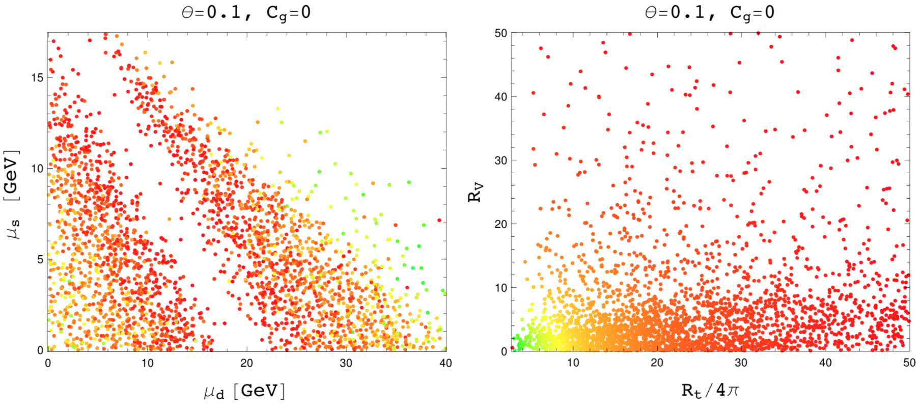
Lower plots: regions allowed by the no-tachyon requirement. The colours correspond to different values of . We have also required that and .
The points corresponding to spectra that are free of tachyons are shown in the lower panels of Fig. 8, where we also restricted
| (108) |
The colours discriminate points depending on how close they are to small ratios, or more precisely we give the same colours to points with the same value of . We see that, as expected, most of the points fill the triangle below the line we identified before. The white band that is missing in the middle, however, is not ruled out by tachyons but by our requirement of small ratios, i.e. it’s a region where NDA is significantly violated. In fact most points are red around this band.


Finally, in Fig. 9 we show correlations between the various mass eigenstates, for the pseudo-scalars ––, for the scalar triplet, for the doubly charged and for the singly charged. The colours keep track of the dominant components of the state in the horizontal axes in terms of the gauge eigenstates, as indicated in the caption. From the top row, relative to the three pseudo-scalars, we see that all the states are lighter than GeV when they are dominantly singlet, in particular the heaviest one, , is always in the range – GeV. This implies that the whole spectrum is light as long as the singlet is the heaviest state. The second row of plots, showing the correlation between the pseudo-scalars and the neutral scalar , highlights a more interesting correlation: the neutral triplet is always degenerate with the mass eigenstate that is dominantly custodial singlet in yellow. Note that the exact equality we observe here is mainly due to our choice in the scan, as a non-zero value of this parameter will induce a splitting due to gauge loops. This effect can also be seen in Fig. 7 for the custodial case, where all the masses (except the singlet ) would become equal in the limit. A looser correlation can be observed between the triplet and the mostly singlet mass eigenstate (red). The bottom row shows correlations among the charged states: we see again a nice correlation between the doubly charged state and the singly charged eigenstate that is mainly from the triplet in blue, even though there are points that lie outside of the line.
In general, a remarkable feature of this model is the presence of light states, whose mass can be as low as GeV, even though we have fixed TeV in the scan. This situation makes the model very promising for searches of new light scalars at the LHC in direct production, or via decays of the top partners [44].
6 General vacuum
The remaining option to eliminate the tadpole of the -field is to allow for a more general vacuum than the one defined in Section 2. Following this approach, one is not forced anymore to require a precise cancellation among the parameters in the potential in order to set the tadpole to zero. Thus, instead of a relation between the parameters, one of them is simply traded with an additional misalignment angle, that we shall denote as . Let us remark that, contrary to what is usually done in elementary models containing triplets, such as the Georgi-Machacek model [15], it is not possible here to generate a custodial symmetric VEV for the triplets (i.e. misalignment). Firstly, this is due to the intrinsic CP-parity carried by the scalars, as discussed in Section 3.2: only the custodial triplet contains a CP-even neutral scalar along which a misalignment can be generated without violating CP. We stress again that a misalignment along any other direction, corresponding to a custodial singlet, would break CP spontaneously. Secondly, a misalignment along the custodial singlet automatically generates a tadpole for the five-plet field , which can only be removed by giving it a VEV (barring exact cancellations between different operators).
The misalignment matrix , defined in Eq. (123) needs to be generalised as follows
| (109) |
where the two generators are given explicitly in Appendix A.1. However, a more convenient parametrisation can be used by observing that the two generators corresponding to the Higgs and neutral triplet directions, together with their commutator, form a algebra [9]:
| (110) |
where the unbroken generator has the following matrix representation:
| (111) |
The generators , given in Appendix A.2, together with and the six generators , provide a complete adjoint representation of the unbroken group on the vacuum . As a consequence of the group structure elucidated above, the vacuum alignment matrix can be conveniently re-parameterised as
| (112) |
where
| (113) |
The explicit form of is given in Appendix A.1. Thus, the linearly transforming pion matrix reads [9]
| (114) |
where is defined on the Higgs vacuum, Eq. (7). As discussed in Ref. [9], the rotation acts on the pion matrix as a mere change of basis, due to the fact that the generator is not broken by the vacuum . Here, we choose to work in the basis where the pion matrix is given by
| (115) |
with given in Eq. (9). In this basis, the field we call has couplings close to the ones of the doublet, while matches approximately the custodial triplet. We remind the reader that the misalignment by the angles and induces a mismatch between the pNGBs and gauge eigenstates.
The masses of the EW gauge bosons have now the following expressions
| (116) |
which gives a tree-level correction to the parameter (the Weinberg angle is not affected at tree-level):
| (117) |
which vanishes either for or for . Also, we remark that for and for , and that it is symmetric under change of sign of . The mass of the top quark is also modified in the new vacuum, but its explicit form depends on the chosen spurions. Here we will focus on the anti-symmetric irrep of as in Section 5, for which it reads:
| (118) |
Besides the tree level correction to the parameter, the new vacuum alignment also modifies the couplings of the would-be Higgs to , and tops, in a non-custodial way. We define the modified couplings with respect to the SM ones as
| (119) |
where is defined by matching the expression of the mass to the SM formula, yielding
| (120) |
and . For the , we obtain
| (121) |
The corresponding expressions for and top are more complicated, and we report them in Appendix A.1. In the limit , where the vacuum is misaligned along the Higgs direction only, we recover the familiar expression while the coupling of the triplet vanishes. On the contrary, for , where the vacuum is only misaligned along the triplet, while the coupling of vanishes. This confirms our expectation that, in the chosen basis, matches the doublet and the custodial triplet.
From Eq. (117) we observed that vanishes for , besides the obvious region near vanishing triplet misalignment . It is, therefore, tantalising to think that such a large region may be still allowed by the Higgs data and by precision tests. The most recent determination of the parameter gives [45], where the fit is marginalised on contributions to other oblique observable such as the parameter. Thus, we will impose a bound on at , which gives the following range: . This is but a rough estimate of the impact of electroweak physics in this model, because at one loop level additional contributions will emerge coming from the modifications of the Higgs couplings and from loops of heavier resonances. For examples of this kind of calculations in other models, we refer the reader to Refs [46, 47, 12]. A detailed analysis of this issue is, however, beyond the scope of this paper, because it heavily relies on the details of the model. One interesting feature is that corrections to the parameters are typically positive [48, 49, 35, 50], and due to the correlation in the EW fit, a positive contribution to (i.e. ) is welcome as it may push the model back into the allowed region [51]. In the model under study, this happens for . It is the deviation on the couplings of the Higgs that will tell us if such a region is still viable.
A mixing between the two scalars and is always generated, while the details depend on the representation of the top spurions and on the free parameters in the pNGB potential. As an example, in Appendix A.5 we briefly discuss the case of the anti-symmetric. Here, however, we simply introduce an angle that rotates the basis into the mass eigenstate one , defined as follows
| (122) |
where we allow to span . Note that both mass eigenstates, and , can, in principle, be identified with the GeV scalar observed at the LHC. The modifications to the Higgs coupling depend on three parameters: the two misalignment angles – and the mixing angle . To compare with the most recent LHC results, we will adopt a very conservative approach and only compare with the most direct available measurements. The reason is that in general additional contribution to the Higgs couplings will arise from loops, which will be especially relevant for the loop induced couplings to gluons and photons. Thus, we need to disentangle the impact of the precise determination of such couplings, via the production rate and the di-photon decay, from the determination of the couplings to ’s and tops. For the couplings to gauge bosons, the most recent measurements at the LHC provide errors of about [52, 53, 54, 55], thus we will conservatively allow a variation of about . For the top coupling, we use the direct measurement coming from the observation of the associated production [56, 57], which gives an error of about on the coupling, thus we show a band of about at . As a first exploration, we show in Fig. 10 the deviations for the doublet (left plot) and triplet (middle plot) for vanishing mixing, and the same for a small mixing angle (right plot). We allow couplings with flipped signs, shown with lighter colours in the plot. The region where all Higgs couplings are compatible with the measurement is thus compared to the most recent best fit of the parameter, with the region within the black lines. We see that the bound on provides an upper limit on for small , while an upper bound on around comes from the top coupling. This is an example of the importance of a direct measurement of the top coupling in CH models. As expected, for a pure triplet there is no region where the Higgs couplings can match the experimental results, while the plot on the right shows that increasing the mixing angle tends to shift the region matching the Higgs couplings outside of the band allowed by the parameter.
In Fig. 11 we show the same allowed regions for fixed values of . For small , as shown in the left plot, besides a limit on coming from , the Higgs couplings to vectors give a bound on the mixing angle of roughly . In the middle and right plots, we show values of close to , where the contribution to is small. For values below , a small region is still allowed by the Higgs couplings, however remaining marginal as it always entails large deviations to the couplings. It also corresponds to negative mixing angles, and it shrinks to a point for . The right plot shows a value above , where a positive contribution to is obtained. However, the values of the would-be Higgs completely exclude this case, as there is no overlap between the allowed regions of the various couplings.
7 LHC phenomenology
As we have seen in the previous sections, apart from the singlet, the light scalar content of the CH model is the same as that of the Georgi-Machacek model [15, 16], GM for short in the remainder of this section. The LHC phenomenology, therefore, shares some common features to the widely studied one of the GM, see Refs [58, 59, 60] and references therein. There are, however, important differences between GM and its composite counterpart: the main one, already highlighted in Section 3.2, is the fact that the CP properties of the triplets are exchanged. Namely, it is the neutral component of the custodial triplet that is CP-even, while the others (including the singlet) are CP-odd. This property can be determined thanks to the fermionic underlying theory. As a consequence, the custodial singlet VEV of the triplets is forbidden in CP-conserving cases, thus a three level coupling of the new scalars to two massive gauge bosons, and , are not generated. We remark that the presence of such couplings plays a leading role in the GM phenomenology, as it allows for single production of the scalars via Vector Boson Fusion (VBF) with further decays in di-bosons [58]. In particular, a benchmark scenario has been identified, for which the fiveplet is the lightest state of the spectrum, thus providing a motivation for scalar di-boson interpretations of LHC searches [61]. This benchmark, as already stressed, is however not allowed in the CH model, where couplings to a pair of gauge bosons are only generated at one loop level by the WZW anomaly and thus yield negligibly small cross sections. The leading production mode for the new composite scalars is, therefore, pair production via gauge interactions, which is dominated by Drell-Yan processes [62, 63].
Couplings to fermions are more model sensitive, as they crucially depend on the origin of the SM fermion masses in the CH model. One difference with respect to the GM model is that couplings of the five-plet to top and bottom quarks are present in some cases, depending on the operator that generates the top mass, while the five-plet is fermiophobic in the GM model. We refer to Section 3.1 for model details. Note, nevertheless, that all fermion couplings are suppressed by , thus they tend to be small. There is also a special case, for top partners in the adjoint of , where all linear couplings of the pNGBs to the top and bottom vanish. Note that the presence of couplings to tops would induce a coupling to gluons, at one loop level, for the neutral (pseudo-)scalars, thus allowing for single production via gluon fusion. If the couplings of the light quarks and leptons are also generated via FPC, the same rules apply as for the top. There is also the other possibility that their couplings are generated by direct bilinear interactions with the strong dynamics, as in Ref. [64]. In this case, the structure of the couplings is more similar to the GM case, as shown in Appendix A.6, as only the five-plet remains fermiophobic. Those couplings would, however, be suppressed by the small Yukawa couplings.
The presence of a doubly-charged state has been identified as a crucial feature of this model since the beginning [15], as it potentially leads to low background final states with same-sign leptons [58, 59]. This signature is also present in the composite model, as the doubly charged scalar, , can only decay in final states that contain two same-sign (virtual) ’s. The main decays are thus into a pair, or into a singly charged state . This pattern matches with the GM case [59]. However, the fact that the coupling is induced by an anomaly (thus being loop suppressed) and suppressed by [15] implies that the cascade decays are always preferred, as long as the mass splitting is large enough. Furthermore, the decays of the singly charged and neutral states into gauge bosons are also induced by the anomaly, implying that final states with photons are equally probable as final states with massive gauge bosons, contrary to the GM case where the couplings involving photons are loop induced [60]. 99 9 The high probability of finding photons in the final state is also enhanced by the fact that the only gauge-invariant WZW coupling of the triplets is of the form , thus it always contains a hypercharge gauge field. Finally, it is always possible to add a direct lepton-number violating bilinear coupling of the triplets to leptons, as shown in Appendix A.6. If the vacuum has a very small misalignment along the triplet, as studied in Section 6, this would lead to a composite type-II see-saw mechanism [65]. From the phenomenology side, the presence of this coupling is very important, as it would allow unsuppressed tree-level decays of the doubly charged scalar into a resonant pair of same-sign leptons [66].
To summarise, the main differences between the CH model and GM are:
- i)
The main production mechanism is pair production via Drell-Yann, as the couplings of a single pNGB to vector bosons are suppressed, being generated by the WZW anomaly. In the GM model, on the contrary, they are induced at tree level by the custodial-invariant -triplet VEV.
- ii)
The couplings to fermions depend on the irrep of the top partners and origin of light fermion masses. In general, the couplings are suppressed by , and they vanish for top partners in the adjoint. The five-plet is not always fermiophobic.
- iii)
Decays to a pair of gauge bosons, of which at least one is a photon, are abundant, as all such couplings are generated by loops. Thus, final states with photons are common for any mass of the scalars. In GM, couplings to photons are loop induced thus relevant only for very low masses below or .
To quantify the above statements, we studied in some more detail a benchmark scenario, which gives rather typical predictions. As we already stressed, the spectra follow a universal pattern, independently of the specific top partner representation, if we limit ourselves to viable models with LO potential. We thus choose to study the model with adjoints, for which the couplings to tops vanish for all pNGBs. The spectrum is shown in Fig. 2, as we also chose in our numerical study. We computed the pair production cross sections via Drell-Yann using our own implementation of the model within the Feynrules package [67], and using the UFO output to generate diagrams and cross sections via MADGRAPH5_aMC@NLO [68]. A more accurate determination of the cross sections, including QCD NLO effects, can be found in Refs [62, 63]. In the top row of Fig. 12 we show the result as a function of the mass for the dominant pair production of doubly charged states, at the LHC Run-II energy and for the projected energy of a future high-energy LHC option. We recall that in this model the mass depends on the parameter , the coefficient of the gauge contribution to the pNGB masses. The doubly charged scalar can decay either into same-sign ’s, or chain decay to a singly-charged scalar plus a virtual . The branching ratios (BRs) are shown in the lower row of Fig. 12, which shows how the final state dominates only for small masses below – GeV. The singly charged state further decays to gauge boson pairs via the anomaly, with a probability of about – approximately flat in the considered range of – of having a photon in the final state.
Lower plots: Branching ratios for the and pNGBs, as functions of their masses. For the BRs of , stands for both and .
The same-sign dilepton (SSL) rate of the doubly charged scalar can be estimated to be , where (and we include leptonic decays of the tau). Thus, roughly 12% of the pair production events yield SSL final states, for cross sections of roughly fb for the smallest mass in our benchmark scenario. The low mass range may, therefore, be accessible to LHC Run-II searches based on SSL, like for instance in Refs [69, 70, 71, 72]. At higher masses, above GeV, decays involving photons become very abundant: using the BRs from Fig. 12, we see that pair production events with two photons in the final state occur around 60% of the times. This means that a new search based on hard photons may be more effective in covering this mass range.1010 10 For an analysis of final states featuring several photons using LHC data, see Ref. [73]. We leave a detailed study of the SSL recast and photon signature for future work. Finally we should mention that, in presence of a Majorana coupling to leptons, resonant decays are also possible, leading to a well-studied signature [66]. To conclude the discussion, in Table 4, we provide some specific numbers for two benchmark points, based on and .
| Process | @13TeV (fb) | @27TeV (fb) | ||
|---|---|---|---|---|
| 0.91 | 0.12 | 5.1 | 0.16 | |
| 0.10 | 0.014 | 0.58 | 0.12 | |
| Masses (GeV) | ||||
| 1112.2 | 853.6 | – | – | |
| 538.0 | 783.2 | – | – | |
| 532.2 | 742.2 | – | – | |
| 538.0 | 782.8 | – | – | |
| 537.8 | 781.6 | – | – | |
| 533.2 | 749.1 | – | – | |
| 538.7 | 787.6 | – | – | |
| BR | ||||
| 0.95 | 0.003 | – | – | |
| 0.03 | 0.67 | – | – | |
| 0.01 | 0.22 | – | – | |
| 0.004 | 0.11 | – | – | |
| 0.79 | 0.78 | – | – | |
| 0.21 | 0.22 | – | – | |
8 Conclusions and outlook
In this work, we illustrated some key features of the composite Higgs model, which was first introduced in [7]. The pNGB spectrum resembles that of the Georgi-Machacek model [15, 16] by the presence of 3 triplets related by the custodial symmetry. We characterise the model by studying not only the embedding of the electroweak symmetry and its breaking, but also the explicit breaking of the symmetry using the spurion formalism. For the top quark we used the paradigm of partial compositeness and considered embeddings transforming under complete two-index representations of . This choice is backed up by realistic models based on gauge-fermion underlying theories. For light quarks and leptons, the mass can be generated either by partial compositeness or by direct bilinear couplings, generated at a higher energy scale than the top ones. We classified all the operators at leading order in the chiral expansion contributing to the top mass (Yukawa) and to the pNGB potential. We then studied their effect on the vacuum stability and pNGB spectra, thus largely extending the work of Ref. [27]. We present the first comprehensive analysis of the properties of this class of models.
We obtained the most general form of the Yukawa interactions between the pNGBs and the top and (left-handed) bottom quarks, showing that, for general embeddings, the couplings of the Higgs and non-Higgs pNGBs are highly correlated. The linear couplings, in fact, are governed in some cases by only one, two or three coefficients, depending on the operator(s) generating the top mass.
We then performed the same general analysis for the potential, and analysed the effect of each operator in the vacuum that has been misaligned along the Higgs direction only. We showed that a misalignment along any custodial singlet direction is forbidden by CP invariance, thus proving that the custodial preserving triplet VEV allowed in the elementary Georgi-Machacek model is not allowed in the CP-conserving composite version. The general analysis of the LO potential led us to identify a few viable scenarios, satisfying the requirements of vacuum misalignment together with the absence of a tadpole for the CP-even pNGB . The misalignment along the triplet needs to be suppressed in order to avoid dangerous corrections to the value of the parameter, and also for consistency with the choice of the Higgs vacuum. The three models correspond to embedding both the left- and right-handed tops into the adjoint of , or embedding the left-handed in the anti-symmetric or the right-handed in the symmetric (and the other in the adjoint). In all other cases, a triplet tadpole is inevitable, thus inducing a more general vacuum misalignment that is highly constrained by electroweak precision tests. In studying the scalar spectra for the three allowed cases, we found a universal pattern related to the transformation properties of the pNGBs under the custodial symmetry. Remarkably, the gauge singlet always receives a negative contributions from loops of gauge bosons as opposed to the rest of the scalars, except in the one case outlined at the end of Sec. 4.3. Moreover, the presence of tachyons often largely restricts the available parameter space, signalling a wrong choice for the minimum.
The case of the anti-symmetric representation offers an example of NLO potential, and we have shown that a limit exists in which the custodial symmetry is restored, at least at the level of the spectrum. The pNGB masses show, however, a different pattern than in the LO cases, which we studied in detail. A common feature, very promising for the LHC phenomenology, is that pNGB masses below 1 TeV are always allowed, even when the condensation scale is in the multi-TeV range.
Finally, we also briefly discuss the LHC phenomenology of the non-Higgs pNGBs, highlighting the differences with respect to the Georgi-Machacek model. Besides the spectrum, it is remarkable the absence of tree-level couplings of the non-Higgs pNGBs to gauge bosons, which thus reduces single production at colliders. The main production mode is, therefore, production in pairs, via gauge interactions. Furthermore, the fact that couplings to gauge bosons are generated by topological anomalies implies that decay final states with photons are very probable, and even dominant, thus providing a new signature with hard photons. Couplings to fermions are model dependent, and, contrary to the elementary case, they can be set to zero in the adjoint-adjoint case. In other cases, including direct bilinear couplings to the strong dynamics, they are always generated. It turns out that there exist cases where the five-plet is not fermiophobic. We leave a more detailed study of the LHC phenomenology for future work. Besides the direct pair production that we discuss here, another interesting production mode derives from the decays of the top partners, if they are light enough to be produced at the LHC, or at future higher energy hadron colliders.
Acknowledgements
We thank Daniele Barducci for suggestions concerning the Feynrules implementation of the model. AD is partially supported by the Institut Univérsitaire de France. AD and GC also acknowledge partial support from the Labex-LIO (Lyon Institute of Origins) under grant ANR-10-LABX-66 (Agence Nationale pour la Recherche), and FRAMA (FR3127, Fédération de Recherche “André Marie Ampère”). AA thanks the IPNL for hospitality during the completion of this work.
Appendices
Appendix A Details of the model
A.1 Choice of the vacuum
The misalignment rotation, is generated by the generator associated to the VEV of the Higgs, , and equals
| (123) |
The Higgs vacuum thus reads:
In Section 6 we introduced a more general rotation , which is also misaligned along the generator , corresponding to the neutral custodial triplet field , given by:
We found that , with
In this new vacuum, the couplings of the scalars and to and top, normalised to the SM values, read:
| (134) | |||||
| (135) | |||||
| (136) | |||||
| (137) |
In the limit , we recover the results in the Higgs vacuum, namely and for the vectors, and and for the top. In the limit , where the vacuum is misaligned along the triplet, the couplings of to vectors vanish while and . In the same limit, the coupling diverges due to the fact that the mass of the top vanishes.
A.2 generators
We list here the missing generators mentioned in Section 6:
A.3 Custodial basis
The real triplet and the complex triplet can be rewritten in terms of the custodial , which is the diagonal of . The bi-triplet decomposes as . The triplet components are mapped to the new basis as:
| (153) |
We recall that , , and .
A.4 Mass term and vacuum alignment
In this paragraph we briefly clarify the link between the choice of the mass matrix for the HFs and the choice of the vacuum, which we mentioned in Section 3.3.2. To this aim, consider a toy model where the only contribution to the pNGB potential comes from the HF mass term, like in Eq. (51). For , the minimum is at , and it generates the following masses for the Higgs doublet, triplets and singlet :
| (154) |
We clearly see that for , the Higgs doublet squared mass turns negative, thus justifying the expectation that the minimum of the potential would be moved away fro zero. However, the above expressions show that the singlet becomes tachyonic for less negative values of , i.e. . This implies that the vacuum needs to be misaligned along the singlet even before the Higgs direction is destabilised.
We will show now that this destabilisation along the singlet, that occurs for negative , calls for choosing the second inequivalent EW preserving vacuum
| (155) |
which, compared to the one in Eq. (6), has a minus sign corresponding to the negative singlet squared mass. One can go from the vacuum to the new one with a transformation by the generator associated to (times an overall phase shift):
| (156) |
The relation is, therefore,
| (157) |
Let us now consider a theory with an HF mass term with and . If we define the EW vacuum , all the equations for the vacuum alignment Eq. (51) and (154) would be the same but for a flipped sign in front of . That is, the results are the same as we would obtain for a theory with and around the vacuum . Thus, also for , once the correct EW preserving vacuum is chosen, the theory is well defined at the minimum . This analysis proves that the HF term alone cannot trigger EWSB. As a final remark, we would like to remind that the broken generator bases in the two vacua are not the same, thus one needs to define a new pNGB basis on , which is related to the basis for in Eq.(9) by
| (158) |
A.5 Potential in the general vacuum for top anti-symmetric spurions
Restricting to the case of the - top partner irrep, the scalar potential generated by the NLO operators, given in Eq.(91), takes the following simple form:
| (159) |
with
| (160) |
Only five of the ten coefficients given above are linearly independent, being related by the following five linear constraints:
| (161) |
Note that, as opposed to the case of the -vacuum, terms proportional to and now also appear in the potential. By looking at the explicit form of the matrix it can be argued that Eq. (159) already gives the most general expansion in , since the operators generating the potential have four insertions of , and the latter only contains trigonometric functions of that can be re-expressed in terms of and (up to unimportant constant shifts).
A.6 Effective Yukawa couplings and type-II see-saw
For completeness, we list here the effective Yukawa couplings between the SM fermions and the strong dynamics, which may be responsible for generating the masses of the light fermions, while PFC is responsible for the top mass [64]. We define the projectors on the pNGB matrix such that
| (162) |
where is any of the pNGB fields. This will allow us to define gauge-invariant couplings between the pNGB matrix and the SM fermions.
Up-type fermions
For up-type quarks, the effective Yukawa couplings read
| (163) |
where, up to linear pNGB terms, the traces read:
| (164) | |||||
| (165) |
The up-type fermion mass, thus, reads
| (166) |
and couplings to all pNGBs are generated, except for the five-plet. This result matches the ones for the elementary Georgi-Machacek model.
Down-type fermions
For down-type quarks and charged leptons, the effective Yukawa couplings read
| (167) |
where, up to linear pNGB terms, the traces read:
| (168) | |||||
| (169) |
The down-type fermion mass, thus, reads
| (170) |
and, again, couplings to all pNGBs are generated, except for the five-plet.
Neutrino masses and type-II see-saw mechanism
Due to the presence of a charged triplet in the pNGB spectrum, direct couplings to a leptonic operator is allowed, in analogy to what is done in type-II see-saw models [65]. This operator can be generated either by a direct bi-linear coupling or by integrating out fermionic partners in partial compositeness, thus allowing a direct Majorana mass for the left-handed neutrinos. For the former case, the effective couplings read:
| (171) |
with
| (172) | |||||
| (173) | |||||
| (174) |
The constant term in the first line indicates that a mass for the neutrinos is generated, and the proportionality to suggests that this is equivalent to the dimension-5 Weinberg operator in the SM. If this term were absent, as it may be in case of partial compositeness, a Majorana mass term may be generated by giving a small VEV to the triplet . Also, this coupling can potentially generate sizeable couplings of the five-plet to leptons, in particular for the doubly charged, thus allowing decays at tree level.
Appendix B Proof of equivalence between our basis of invariant operators and a basis of invariant ones
Instead of constructing explicitly a basis of invariant operators following the procedure defined in Refs [35, 36], we will prove the equivalence of the two bases by tracing the contribution of the various components inside the invariant operators defined in the main text.
Firstly, we observe that for each pair of spurions in Table 1 there exists a single component in common. Thus, operators that contain two different spurions can only correspond to a single operator constructed in terms of invariants. The same is true for operators containing only the anti-symmetric. In the following we will therefore only focus on operators containing two adjoints, or two symmetric (and/or the conjugate) irreps.
For the adjoint, the only LO template operator has the form
| (175) |
To isolate the contribution of the two components, we first observe that the adjoint spurions can be mapped into a 2-index irrep of by multiplying them by the pNGB matrix , namely taking the combination (and for the conjugate). The symmetric and anti-symmetric components can thus be extracted as follows:
| (176) |
We can construct, therefore, two operators from the template in Eq. (175):
| (177) | |||||
The last line thus shows that the two operators constructed with the symmetric and anti-symmetric components of the adjoint are equivalent, up to a pNGB-independent operator that only contains the trace of the two spurions. Note that such trace vanishes for the top mass operator in Section 3.1, while it simply gives a constant term in the potential in Section 3.3.
For the symmetric spurion, and its conjugate irrep, it is most convenient to map it into a matrix transforming like the adjoint, (and ). The traceless component of such matrix will contain the symmetric component, as this is the only irrep in common to the adjoint, while the remaining term corresponds to the singlet component. We can thus decompose it as follows:
| (178) |
and similarly for the conjugate spurion. From the above decomposition, it is clear that the double-trace operators will only pick up the singlet component of the symmetric (and conjugate) spurions. On the other hand, the single-trace operator gives
| (179) |
and similarly for the operator containing the conjugate. This shows that the operator constructed in terms of the symmetric component is equivalent to a linear combination of the single and double trace operators.
The considerations above show that a basis constructed in terms of invariants at LO is equivalent to a basis constructed in terms of invariants.
References
- (1) ATLAS collaboration, R. D. Harrington, “Observation of an excess of events in the Higgs boson search in ATLAS,”Nucl. Phys. Proc. Suppl. 234 (2013) 15–20.
- (2) CMS collaboration, S. Chatrchyan et al., “Observation of a new boson with mass near 125 GeV in pp collisions at = 7 and 8 TeV,”JHEP 06 (2013) 081, [1303.4571].
- (3) G. Degrassi, S. Di Vita, J. Elias-Miro, J. R. Espinosa, G. F. Giudice, G. Isidori et al., “Higgs mass and vacuum stability in the Standard Model at NNLO,”JHEP 08 (2012) 098, [1205.6497].
- (4) D. Buttazzo, G. Degrassi, P. P. Giardino, G. F. Giudice, F. Sala, A. Salvio et al., “Investigating the near-criticality of the Higgs boson,”JHEP 12 (2013) 089, [1307.3536].
- (5) D. B. Kaplan and H. Georgi, “SU(2) x U(1) Breaking by Vacuum Misalignment,”Phys. Lett. 136B (1984) 183–186.
- (6) G. Cacciapaglia and F. Sannino, “Fundamental Composite (Goldstone) Higgs Dynamics,”JHEP 04 (2014) 111, [1402.0233].
- (7) M. J. Dugan, H. Georgi and D. B. Kaplan, “Anatomy of a Composite Higgs Model,”Nucl. Phys. B254 (1985) 299–326.
- (8) T. Ma and G. Cacciapaglia, “Fundamental Composite 2HDM: SU(N) with 4 flavours,”JHEP 03 (2016) 211, [1508.07014].
- (9) C. Cai, G. Cacciapaglia and H.-H. Zhang, “Vacuum alignment in a composite 2HDM,” 1805.07619.
- (10) J. Serra, “Beyond the Minimal Top Partner Decay,”JHEP 09 (2015) 176, [1506.05110].
- (11) A. Banerjee, G. Bhattacharyya and T. S. Ray, “Improving Fine-tuning in Composite Higgs Models,”Phys. Rev. D96 (2017) 035040, [1703.08011].
- (12) A. Arbey, G. Cacciapaglia, H. Cai, A. Deandrea, S. Le Corre and F. Sannino, “Fundamental Composite Electroweak Dynamics: Status at the LHC,”Phys. Rev. D95 (2017) 015028, [1502.04718].
- (13) E. Katz, A. E. Nelson and D. G. E. Walker, “The Intermediate Higgs,”JHEP 08 (2005) 074, [hep-ph/0504252].
- (14) G. Ferretti, “UV Completions of Partial Compositeness: The Case for a SU(4) Gauge Group,”JHEP 06 (2014) 142, [1404.7137].
- (15) H. Georgi and M. Machacek, “Doubly charged Higgs bosons,”Nucl. Phys. B262 (1985) 463–477.
- (16) M. S. Chanowitz and M. Golden, “Higgs Boson Triplets With M () = M () ,”Phys. Lett. 165B (1985) 105–108.
- (17) R. Campbell, S. Godfrey, H. E. Logan and A. Poulin, “Real singlet scalar dark matter extension of the Georgi-Machacek model,”Phys. Rev. D95 (2017) 016005, [1610.08097].
- (18) D. B. Kaplan, “Flavor at SSC energies: A New mechanism for dynamically generated fermion masses,”Nucl. Phys. B365 (1991) 259–278.
- (19) J. Barnard, T. Gherghetta and T. S. Ray, “UV descriptions of composite Higgs models without elementary scalars,”JHEP 02 (2014) 002, [1311.6562].
- (20) G. Ferretti and D. Karateev, “Fermionic UV completions of Composite Higgs models,”JHEP 03 (2014) 077, [1312.5330].
- (21) M. Golterman and Y. Shamir, “Top quark induced effective potential in a composite Higgs model,”Phys. Rev. D91 (2015) 094506, [1502.00390].
- (22) G. Ferretti, “Gauge theories of Partial Compositeness: Scenarios for Run-II of the LHC,”JHEP 06 (2016) 107, [1604.06467].
- (23) E. Bennett, D. K. Hong, J.-W. Lee, C.-J. D. Lin, B. Lucini, M. Piai et al., “Higgs compositeness in Sp(2N) gauge theories ? Determining the low-energy constants with lattice calculations,”EPJ Web Conf. 175 (2018) 08011, [1710.06941].
- (24) E. Bennett, D. K. Hong, J.-W. Lee, C. J. D. Lin, B. Lucini, M. Piai et al., “Sp(4) gauge theory on the lattice: towards SU(4)/Sp(4) composite Higgs (and beyond),”JHEP 03 (2018) 185, [1712.04220].
- (25) V. Ayyar, T. DeGrand, M. Golterman, D. C. Hackett, W. I. Jay, E. T. Neil et al., “Spectroscopy of SU(4) composite Higgs theory with two distinct fermion representations,”Phys. Rev. D97 (2018) 074505, [1710.00806].
- (26) V. Ayyar, T. Degrand, D. C. Hackett, W. I. Jay, E. T. Neil, Y. Shamir et al., “Baryon spectrum of SU(4) composite Higgs theory with two distinct fermion representations,”Phys. Rev. D97 (2018) 114505, [1801.05809].
- (27) M. Golterman and Y. Shamir, “Effective potential in ultraviolet completions for composite Higgs models,” 1707.06033.
- (28) T. Alanne, N. Bizot, G. Cacciapaglia and F. Sannino, “Classification of NLO operators for composite-Higgs models,” 1801.05444.
- (29) L. Vecchi, “The Natural Composite Higgs,” 1304.4579.
- (30) F. Sannino, A. Strumia, A. Tesi and E. Vigiani, “Fundamental partial compositeness,”JHEP 11 (2016) 029, [1607.01659].
- (31) G. Cacciapaglia, H. Gertov, F. Sannino and A. E. Thomsen, “Minimal Fundamental Partial Compositeness,” 1704.07845.
- (32) A. Belyaev, G. Cacciapaglia, H. Cai, G. Ferretti, T. Flacke, A. Parolini et al., “Di-boson signatures as Standard Candles for Partial Compositeness,”JHEP 01 (2017) 094, [1610.06591].
- (33) H. Georgi, “Generalized dimensional analysis,”Phys. Lett. B298 (1993) 187–189, [hep-ph/9207278].
- (34) G. Buchalla, O. Catá and C. Krause, “On the Power Counting in Effective Field Theories,”Phys. Lett. B731 (2014) 80–86, [1312.5624].
- (35) R. Contino, “The Higgs as a Composite Nambu-Goldstone Boson,” in Physics of the large and the small, TASI 09, proceedings of the Theoretical Advanced Study Institute in Elementary Particle Physics, Boulder, Colorado, USA, 1-26 June 2009, pp. 235–306, 2011. 1005.4269. DOI.
- (36) J. Mrazek, A. Pomarol, R. Rattazzi, M. Redi, J. Serra and A. Wulzer, “The Other Natural Two Higgs Doublet Model,”Nucl. Phys. B853 (2011) 1–48, [1105.5403].
- (37) J. Wess and B. Zumino, “Consequences of anomalous Ward identities,”Phys. Lett. 37B (1971) 95–97.
- (38) E. Witten, “Global Aspects of Current Algebra,”Nucl. Phys. B223 (1983) 422–432.
- (39) M. E. Peskin, “The Alignment of the Vacuum in Theories of Technicolor,”Nucl. Phys. B175 (1980) 197–233.
- (40) J. Preskill, “Subgroup Alignment in Hypercolor Theories,”Nucl. Phys. B177 (1981) 21–59.
- (41) J. F. Gunion, R. Vega and J. Wudka, “Naturalness problems for rho = 1 and other large one loop effects for a standard model Higgs sector containing triplet fields,”Phys. Rev. D43 (1991) 2322–2336.
- (42) C. Englert, E. Re and M. Spannowsky, “Triplet Higgs boson collider phenomenology after the LHC,”Phys. Rev. D87 (2013) 095014, [1302.6505].
- (43) S. Blasi, S. De Curtis and K. Yagyu, “Effects of custodial symmetry breaking in the Georgi-Machacek model at high energies,”Phys. Rev. D96 (2017) 015001, [1704.08512].
- (44) N. Bizot, G. Cacciapaglia and T. Flacke, “Common exotic decays of top partners,”JHEP 06 (2018) 065, [1803.00021].
- (45) Particle Data Group collaboration, M. Tanabashi et al., “Review of Particle Physics,”Phys. Rev. D 98 (2018) 030001.
- (46) M. Carena, E. Ponton, J. Santiago and C. E. M. Wagner, “Light Kaluza Klein States in Randall-Sundrum Models with Custodial SU(2),”Nucl. Phys. B759 (2006) 202–227, [hep-ph/0607106].
- (47) R. Barbieri, B. Bellazzini, V. S. Rychkov and A. Varagnolo, “The Higgs boson from an extended symmetry,”Phys. Rev. D76 (2007) 115008, [0706.0432].
- (48) M. E. Peskin and T. Takeuchi, “A New constraint on a strongly interacting Higgs sector,”Phys. Rev. Lett. 65 (1990) 964–967.
- (49) J. Hirn and V. Sanz, “A Negative S parameter from holographic technicolor,”Phys. Rev. Lett. 97 (2006) 121803, [hep-ph/0606086].
- (50) G. Panico and A. Wulzer, “The Composite Nambu-Goldstone Higgs,”Lect. Notes Phys. 913 (2016) pp.1–316, [1506.01961].
- (51) C. Grojean, O. Matsedonskyi and G. Panico, “Light top partners and precision physics,”JHEP 10 (2013) 160, [1306.4655].
- (52) CMS collaboration, A. M. Sirunyan et al., “Measurements of properties of the Higgs boson decaying into the four-lepton final state in pp collisions at TeV,”JHEP 11 (2017) 047, [1706.09936].
- (53) CMS collaboration, A. M. Sirunyan et al., “Measurements of properties of the Higgs boson decaying to a W boson pair in pp collisions at 13 TeV,”Submitted to: Phys. Lett. (2018) , [1806.05246].
- (54) ATLAS collaboration, M. Aaboud et al., “Measurement of the Higgs boson coupling properties in the decay channel at = 13 TeV with the ATLAS detector,”JHEP 03 (2018) 095, [1712.02304].
- (55) ATLAS collaboration, M. Aaboud et al., “Constraints on off-shell Higgs boson production and the Higgs boson total width in and final states with the ATLAS detector,”Submitted to: Phys. Lett. (2018) , [1808.01191].
- (56) ATLAS collaboration, M. Aaboud et al., “Observation of Higgs boson production in association with a top quark pair at the LHC with the ATLAS detector,”Phys. Lett. B784 (2018) 173–191, [1806.00425].
- (57) CMS collaboration, A. M. Sirunyan et al., “Observation of H production,”Phys. Rev. Lett. 120 (2018) 231801, [1804.02610].
- (58) C. Englert, E. Re and M. Spannowsky, “Pinning down Higgs triplets at the LHC,”Phys. Rev. D88 (2013) 035024, [1306.6228].
- (59) C.-W. Chiang, A.-L. Kuo and T. Yamada, “Searches of exotic Higgs bosons in general mass spectra of the Georgi-Machacek model at the LHC,”JHEP 01 (2016) 120, [1511.00865].
- (60) C. Degrande, K. Hartling and H. E. Logan, “Scalar decays to , , and in the Georgi-Machacek model,”Phys. Rev. D96 (2017) 075013, [1708.08753].
- (61) H. E. Logan and M. B. Reimer, “Characterizing a benchmark scenario for heavy Higgs boson searches in the Georgi-Machacek model,”Phys. Rev. D96 (2017) 095029, [1709.01883].
- (62) T. Han, B. Mukhopadhyaya, Z. Si and K. Wang, “Pair production of doubly-charged scalars: Neutrino mass constraints and signals at the LHC,”Phys. Rev. D76 (2007) 075013, [0706.0441].
- (63) C. Degrande, K. Hartling, H. E. Logan, A. D. Peterson and M. Zaro, “Automatic predictions in the Georgi-Machacek model at next-to-leading order accuracy,”Phys. Rev. D93 (2016) 035004, [1512.01243].
- (64) G. Cacciapaglia, H. Cai, T. Flacke, S. J. Lee, A. Parolini and H. Serodio, “Anarchic Yukawas and top partial compositeness: the flavour of a successful marriage,”JHEP 06 (2015) 085, [1501.03818].
- (65) E. Ma and U. Sarkar, “Neutrino masses and leptogenesis with heavy Higgs triplets,”Phys. Rev. Lett. 80 (1998) 5716–5719, [hep-ph/9802445].
- (66) A. G. Akeroyd, C.-W. Chiang and N. Gaur, “Leptonic signatures of doubly charged Higgs boson production at the LHC,”JHEP 11 (2010) 005, [1009.2780].
- (67) A. Alloul, N. D. Christensen, C. Degrande, C. Duhr and B. Fuks, “FeynRules 2.0 - A complete toolbox for tree-level phenomenology,”Comput. Phys. Commun. 185 (2014) 2250–2300, [1310.1921].
- (68) J. Alwall, R. Frederix, S. Frixione, V. Hirschi, F. Maltoni, O. Mattelaer et al., “The automated computation of tree-level and next-to-leading order differential cross sections, and their matching to parton shower simulations,”JHEP 07 (2014) 079, [1405.0301].
- (69) CMS collaboration, V. Khachatryan et al., “Search for supersymmetry in events with a photon, a lepton, and missing transverse momentum in pp collisions at 8 TeV,”Phys. Lett. B757 (2016) 6–31, [1508.01218].
- (70) CMS collaboration, A. M. Sirunyan et al., “Search for physics beyond the standard model in events with two leptons of same sign, missing transverse momentum, and jets in proton–proton collisions at ,”Eur. Phys. J. C77 (2017) 578, [1704.07323].
- (71) ATLAS collaboration, M. Aaboud et al., “Search for supersymmetry in final states with two same-sign or three leptons and jets using 36 fb-1 of TeV collision data with the ATLAS detector,”JHEP 09 (2017) 084, [1706.03731].
- (72) ATLAS collaboration, M. Aaboud et al., “Search for photonic signatures of gauge-mediated supersymmetry in 13 TeV collisions with the ATLAS detector,”Phys. Rev. D97 (2018) 092006, [1802.03158].
- (73) D. Barducci, S. De Curtis, M. Redi and A. Tesi, “An almost elementary Higgs: Theory and Practice,”JHEP 08 (2018) 017, [1805.12578].