跳到论文正文
W Papers独立论文阅读器 arXiv:1808.10065 论文正文 计算阅读时间 · 0%
引用这篇论文根据当前论文元数据生成,正式投稿前建议核对。


License: arXiv.org perpetual non-exclusive license
arXiv:1808.10065v1 [math.ST] 29 Aug 2018

Quadratic Discriminant Analysis under Moderate Dimension

Qing Yang11 1 Postdoctoral Researcher, Department of Statistics, Purdue University, West Lafayette, IN 47906. (Email: qyang1@e.ntu.edu.sg).    Guang Cheng22 2 Corresponding Author. Professor, Department of Statistics, Purdue University, West Lafayette, IN 47906. (E-mail: chengg@purdue.edu). Research Sponsored by NSF DMS-1712907, DMS-1811812, DMS-1821183, and Office of Naval Research, (ONR N00014-18-2759).
Abstract

Quadratic discriminant analysis (QDA) is a simple method to classify a subject into two populations, and was proven to perform as well as the Bayes rule when the data dimension pp is fixed. The main purpose of this paper is to examine the empirical and theoretical behaviors of QDA where pp grows proportionally to the sample sizes without imposing any structural assumption on the parameters. The first finding in this moderate dimension regime is that QDA can perform as poorly as random guessing even when the two populations deviate significantly. This motivates a generalized version of QDA that automatically adapts to dimensionality. Under a finite fourth moment condition, we derive misclassification rates for both the generalized QDA and the optimal one. A direct comparison reveals one “easy” case where the difference between two rates converges to zero and one “hard” case where that converges to some strictly positive constant. For the latter, a divide-and-conquer approach over dimension (rather than sample) followed by a screening procedure is proposed to narrow the gap. Various numerical studies are conducted to back up the proposed methodology.

Keywords: Misclassification rate; moderate dimension; quadratic discriminant analysis; random matrix theory.

1 Introduction

Suppose we have two pp-variate classes with mean vectors and covariance matrices (𝝁1,Σ1)({\bm{\mu}}_{1},\Sigma_{1}) (class 1) and (𝝁2,Σ2)({\bm{\mu}}_{2},\Sigma_{2}) (class 2) respectively. The aim is to identify to which class a new observation 𝐳{\bf z} belongs, on the basis of two sets of training samples {𝐱1,⋯,𝐱n1}\{{\bf x}_{1},\cdots,{\bf x}_{n_{1}}\} and {𝐲1,⋯,𝐲n2}\{{\bf y}_{1},\cdots,{\bf y}_{n_{2}}\}. This problem has been well studied in the fixed dimensional setting, see [1] for example. Some recent high dimensional studies allow the data dimension pp to be much larger than the sample sizes, but heavily rely on the sparsity or other structural assumptions on the population parameters 𝝁i{\bm{\mu}}_{i} and Σi\Sigma_{i} (i=1,2)(i=1,2). For example, (𝝁2−𝝁1)({\bm{\mu}}_{2}-{\bm{\mu}}_{1}) is sparse or Σi\Sigma_{i}s satisfy special structures such that better estimators (e.g. thresholding, diagonalization) can be constructed – many improvements have been made over the classical classification rules. One may refer to [5, 13, 15, 17, 22, 25] among others for such improvements over the well-known Fisher’s linear discriminant analysis (LDA) when Σ1=Σ2\Sigma_{1}=\Sigma_{2}; and see [7, 14, 20] and [26], to list but a few for the modifications over the quadratic discriminant analysis (QDA) when Σ1≠Σ2\Sigma_{1}\neq\Sigma_{2}.

Despite these recent progress, there has been relatively fewer development for classification in the moderate dimension regime, by which we mean that p/ni→ci∈(0,1)p/n_{i}\rightarrow c_{i}\in(0,1) and there is no structural assumption on the parameters 𝝁i{\bm{\mu}}_{i} and Σi\Sigma_{i}. One exception is moderate-dimensional LDA by [24]. Clearly, their analyses do not apply to QDA that mainly relies on a quadratic form. Another somehow related line is the study of logistic regression that can be used as a classification rule; see [23, 6]. However, these works mostly focused on the inference results on the parameter itself, e.g., log-likelihood ratio test, rather than classification performances. One can also refer to [8, 9, 10, 11, 12, 16, 18] and [19] for other moderate dimensional results in the linear regression models.

It is well known that the state of the art quadratic discriminant rule classifies 𝐳{\bf z} to class 1 if and only if

d1​(𝐳)+log⁡|Σ1|<d2​(𝐳)+log⁡|Σ2|,d_{1}({\bf z})+\log|\Sigma_{1}|<d_{2}({\bf z})+\log|\Sigma_{2}|, (1.1)

where “|A||A|” denotes the determinant of the matrix AA and

di(𝐳)=(𝐳−𝝁i)TΣi−1(𝐳−𝝁i),i=1,2.d_{i}({\bf z})=({\bf z}-{\bm{\mu}}_{i})^{T}\Sigma_{i}^{-1}({\bf z}-{\bm{\mu}}_{i}),\quad i=1,2. (1.2)

We call it “optimal QDA,” which serves as a performance benchmark in our paper. In practice, the population parameters need to be estimated from training samples, leading to what we call as “sample QDA” as follows. That is to say, the new observation 𝐳{\bf z} is classified to class 1 if and only if

D1​(𝐳)+log⁡|S1|<D2​(𝐳)+log⁡|S2|,D_{1}({\bf z})+\log|S_{1}|<D_{2}({\bf z})+\log|S_{2}|, (1.3)

where

D1​(𝐳)=(𝐳−𝐱¯)T​S1−1​(𝐳−𝐱¯),D2​(𝐳)=(𝐳−𝐲¯)T​S2−1​(𝐳−𝐲¯),\displaystyle D_{1}({\bf z})=({\bf z}-\bar{\bf x})^{T}S_{1}^{-1}({\bf z}-\bar{\bf x}),\quad D_{2}({\bf z})=({\bf z}-\bar{\bf y})^{T}S_{2}^{-1}({\bf z}-\bar{\bf y}),
S1=1n1−1​∑i=1n1(𝐱i−𝐱¯)​(𝐱i−𝐱¯)T,S2=1n2−1​∑i=1n2(𝐲i−𝐲¯)​(𝐲i−𝐲¯)T.\displaystyle S_{1}=\frac{1}{n_{1}-1}\sum\limits_{i=1}^{n_{1}}({\bf x}_{i}-\bar{\bf x})({\bf x}_{i}-\bar{\bf x})^{T},\quad S_{2}=\frac{1}{n_{2}-1}\sum\limits_{i=1}^{n_{2}}({\bf y}_{i}-\bar{\bf y})({\bf y}_{i}-\bar{\bf y})^{T}. (1.4)

We next conduct a simple experiment to empirically examine the classification performances of sample QDA when pp is moderately large compared with the sample size. Specifically, we generate n1n_{1} and n2n_{2} samples from two classes Np​(𝟎,𝐈p)N_{p}({\bf 0},{\bf I}_{p}) and Np​(𝟎,2​𝐈p)N_{p}({\bf 0},2{\bf I}_{p}), respectively. Set n1=n2=nn_{1}=n_{2}=n with nn varying from 100100 to 15001500. The misclassification rate is defined as

R=12​[ℙ2|1+ℙ1|2],ℙi|j≜ℙ⁡{classify​𝐳​to​class ​i|𝐳∈class ​j}.R=\frac{1}{2}\left[\mathbb{P}_{2|1}+\mathbb{P}_{1|2}\right],\qquad\mathbb{P}_{i|j}\triangleq\mathbb{P}\{\text{classify}\ {\bf z}\ \text{to}\ \text{class }\ i\ |{\bf z}\in\text{class }\ j\}. (1.5)

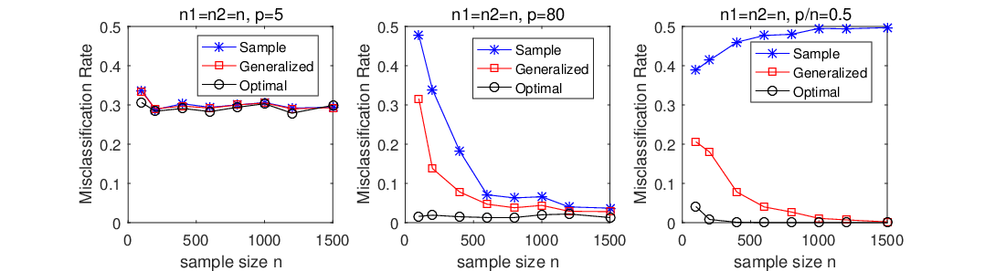
Denote RSR^{S} and ROR^{O} as misclassification rates for sample QDA and optimal QDA** * Throughout this paper, superscripts “O”, “S” and “G” are adopted to denote the values corresponding to the optimal QDA (1.1), the sample QDA (1.3) and our generalized QDA (2.8) introduced later., respectively. From Figure 1 (based on 1000 replications), we observe that the sample QDA matches well with the optimal one when pp is very small compared with nn (the left plot), but the gap between them becomes notable when nn is not significantly large compared with pp (the middle plot) and RSR^{S} even converges to 0.5 (random guessing) when pp is proportional to nn (the right plot). This is an indication of sample QDA’s failure in the moderate-dimensional setting.

Refer to caption
Figure 1: Misclassification rates for two classes Np​(𝟎,𝐈p)N_{p}({\bf 0},{\bf I}_{p}) and Np​(𝟎,2​𝐈p)N_{p}({\bf 0},2{\bf I}_{p}) based on 1000 replications.

The rationale behind the above moderate-dimension phenomenon is simple: the sample mean vectors and sample covariance matrices are no longer consistent in terms of the L2L_{2} norm and the spectral norm, respectively. In fact, a careful analysis of two terms Di​(𝐳)D_{i}({\bf z}) and log⁡|Si|\log|S_{i}| reveals that an extra scaling factor to the former and an extra shift factor to latter need to be introduced to adapt to dimensional effect; see Section 2.1. This leads to a generalized QDA that is built on these two corrected terms; see Section 2.2.

We employ various techniques in the random matrix theory to derive misclassification rates of the generalized QDA, the optimal QDA and the sample QDA in Sections 3.1 and 3.2, without imposing any structural or parametric distribution assumption. This is radically different from the QDA results in the literature that were developed based on normal distribution. In comparison, we only need a finite fourth moment condition on the data, which we believe to be the weakest moment assumption. This can be achieved mainly because we figure out the limiting point of an average squared diagonal entries of a general inverse sample covariance matrix, as formulated in Proposition A.1. Such a result is new to our knowledge. By comparing the misclassification rates between the generalized QDA and the optimal one, we find two cases – the “easy” case where the rate difference converges to zero and the “hard” case where the rate difference converges to some strictly positive constant.

Various simulation studies in Section 4.1 support our theoretical conclusions. To narrow the gap in the “hard” case, two divide-and-conquer approaches are proposed in Section 4.2. In contrast with the conventional partition over samples (which is shown not to work in Supplement S1), our methods are conducted over the dimension followed by a screening procedure. Both show significant improvement over the original generalized QDA. Unless otherwise noted, all the main proofs are relegated to Appendix A. Extra theoretical and numerical results are included in the supplementary material.

2 Methodology – Tame the Dimensionality Effect

In this section, we study the performances of Di​(𝐳)D_{i}({\bf z}) and log⁡|Si|\log|S_{i}| in (1.3) under moderate dimension, see Section 2.1, which motivate a dimension adaptive version of QDA in Section 2.2. A set of mild conditions are needed throughout this paper.

Condition 2.1.

[Population] The class 1 has the form 𝐱i=Σ112​𝐱i0+𝛍1{\bf x}_{i}=\Sigma_{1}^{\frac{1}{2}}{\bf x}_{i}^{0}+{\bm{\mu}}_{1}, i=1,⋯,n1i=1,\cdots,n_{1}, where 𝐱i0=(Xi​1,⋯,Xi​p)T{\bf x}_{i}^{0}=(X_{i1},\cdots,X_{ip})^{T} has pp i.i.d centered and standardized components with finite fourth moments, i.e. m4:=𝔼​|Xi​j|4<∞m_{4}:=\mathbb{E}|X_{ij}|^{4}<\infty. The same form applies to class 2, i.e. 𝐲i=Σ212​𝐲i0+𝛍2{\bf y}_{i}=\Sigma_{2}^{\frac{1}{2}}{\bf y}_{i}^{0}+{\bm{\mu}}_{2}. Moreover, there exist cc and CC s.t. 0<c≤λmin​(Σi)≤λmax​(Σi)≤C<∞0<c\leq\lambda_{\min}(\Sigma_{i})\leq\lambda_{\max}(\Sigma_{i})\leq C<\infty, i=1,2i=1,2.

Condition 2.2.

[Dimensionality] p/n1→c1∈(0,1)p/n_{1}\rightarrow c_{1}\in(0,1) and p/n2→c2∈(0,1)p/n_{2}\rightarrow c_{2}\in(0,1).

Condition 2.3.

[Covariance Matrix] The following limits exist

1p​tr​(Σ1​Σ2−1)→M1,1p​∑i=1p[(Σ112​Σ2−1​Σ112)i​i]2→M2,\frac{1}{p}\mathrm{tr}(\Sigma_{1}\Sigma_{2}^{-1})\rightarrow M_{1},\qquad\frac{1}{p}\sum_{i=1}^{p}[(\Sigma_{1}^{\frac{1}{2}}\Sigma_{2}^{-1}\Sigma_{1}^{\frac{1}{2}})_{ii}]^{2}\rightarrow M_{2},
1p​tr​(Σ2​Σ1−1)→M3,1p​∑i=1p[(Σ212​Σ1−1​Σ212)i​i]2→M4,\frac{1}{p}\mathrm{tr}(\Sigma_{2}\Sigma_{1}^{-1})\rightarrow M_{3},\qquad\frac{1}{p}\sum_{i=1}^{p}[(\Sigma_{2}^{\frac{1}{2}}\Sigma_{1}^{-1}\Sigma_{2}^{\frac{1}{2}})_{ii}]^{2}\rightarrow M_{4},
1p​tr​(Σ1​Σ2−1)2→M5,1p​tr​(Σ2​Σ1−1)2→M6.\frac{1}{p}\mathrm{tr}(\Sigma_{1}\Sigma_{2}^{-1})^{2}\rightarrow M_{5},\qquad\frac{1}{p}\mathrm{tr}(\Sigma_{2}\Sigma_{1}^{-1})^{2}\rightarrow M_{6}.
Remark 2.1.

A simple example to understand the limits in Condition 2.3: if Σ1=κ​Σ2\Sigma_{1}=\kappa\Sigma_{2}, κ>0\kappa>0, then M1=κM_{1}=\kappa, M3=1κM_{3}=\frac{1}{\kappa}, M2=M5=κ2M_{2}=M_{5}=\kappa^{2} and M4=M6=1κ2M_{4}=M_{6}=\frac{1}{\kappa^{2}}.

2.1 Dimension distortion of Di​(𝐳)D_{i}({\bf z}) and log⁡|Si|\log|S_{i}|

One observes that the mean values of d1​(𝐳)d_{1}({\bf z}) and d1​(𝐳)d_{1}({\bf z}) in (1.2) are equal when 𝐳{\bf z} is correctly classified irrespective of data dimension, i.e., if 𝐳{\bf z} belongs to class 1, 𝔼​d1​(𝐳)=p\mathbb{E}d_{1}({\bf z})=p and if 𝐳{\bf z} belongs to class 2, 𝔼​d2​(𝐳)=p\mathbb{E}d_{2}({\bf z})=p. However, such an equivalence does not hold for their sample version Di​(𝐳)D_{i}({\bf z}) in (1.4) when pp diverges proportionally to nn.

To be more precise, we derive the following limiting distributions for Di​(𝐳)D_{i}({\bf z}), i=1,2i=1,2. This weak convergence result is also needed in deriving the misclassification rate in Section 3.

Theorem 2.1.

Under Conditions 2.1 and 2.2, if 𝐳{\bf z} belongs to class 1, we have

1p​D1​(𝐳)−p​s0​n→𝐷N⁡(0,(m4−3)​s02+2​s0′).\frac{1}{\sqrt{p}}D_{1}({\bf z})-\sqrt{p}s_{0n}\xrightarrow{D}N\Big(0,(m_{4}-3)s_{0}^{2}+2s^{\prime}_{0}\Big). (2.1)

If 𝐳{\bf z} belongs to class 2, we have

1p​D2​(𝐳)−p​m0​n→𝐷N⁡(0,(m4−3)​m02+2​m0′).\frac{1}{\sqrt{p}}D_{2}({\bf z})-\sqrt{p}m_{0n}\xrightarrow{D}N\Big(0,(m_{4}-3)m_{0}^{2}+2m^{\prime}_{0}\Big). (2.2)

Here “→𝐷\xrightarrow{D}” denotes convergence in distribution, and

s0​n=11−p/n1,m0​n=11−p/n2,s0=11−c1,s0′=1(1−c1)3,m0=11−c2,m0′=1(1−c2)3,s_{0n}=\frac{1}{1-p/n_{1}},\ m_{0n}=\frac{1}{1-p/n_{2}},\ s_{0}=\frac{1}{1-c_{1}},\ s^{\prime}_{0}=\frac{1}{(1-c_{1})^{3}},\ m_{0}=\frac{1}{1-c_{2}},\ m^{\prime}_{0}=\frac{1}{(1-c_{2})^{3}}, (2.3)

where c1c_{1} and c2c_{2} are given in Condition 2.2.

Theorem 2.1 implies that under moderate dimension, D1​(𝐳)≈p​s0​nD_{1}({\bf z})\approx ps_{0n} when 𝐳{\bf z} belongs to class 1 and D2​(𝐳)≈p​m0​nD_{2}({\bf z})\approx pm_{0n} when 𝐳{\bf z} belongs to class 2 (covering the fixed dimensional case, i.e., s0​n=m0​n=1s_{0n}=m_{0n}=1, as a special case). Hence, to counteract the effects of moderate dimension, we need to rescale the quadratic terms in the sample QDA (1.3) as follows

1s0​n​D1​(𝐳)and1m0​n​D2​(𝐳).\frac{1}{s_{0n}}D_{1}({\bf z})\qquad\text{and}\qquad\frac{1}{m_{0n}}D_{2}({\bf z}). (2.4)

A “re-centering” type of dimension correction will be applied to log⁡|Si|\log|S_{i}| in (1.3). Define

𝐗0=(𝐱10,⋯,𝐱n10),𝐱¯0=1n1​∑i=1n1𝐱i0,𝐗¯0=𝐱¯0⋅𝟏n1T,S10=1n1−1​(𝐗0−𝐗¯0)​(𝐗0−𝐗¯0)T.{\bf X}^{0}=({\bf x}_{1}^{0},\cdots,{\bf x}_{n_{1}}^{0}),\quad\bar{\bf x}^{0}=\frac{1}{n_{1}}\sum_{i=1}^{n_{1}}{\bf x}_{i}^{0},\quad\bar{\bf X}^{0}=\bar{\bf x}^{0}\cdot{\bf 1}_{n_{1}}^{T},\quad S_{1}^{0}=\frac{1}{n_{1}-1}({\bf X}^{0}-\bar{\bf X}^{0})({\bf X}^{0}-\bar{\bf X}^{0})^{T}. (2.5)

Here 𝟏n1{\bf 1}_{n_{1}} is a n1n_{1}-variate vector with all entries being ones. Notations for class 2 can be defined similarly. For example, S20=1n2−1​(𝐘0−𝐘¯0)​(𝐘0−𝐘¯0)TS_{2}^{0}=\frac{1}{n_{2}-1}({\bf Y}^{0}-\bar{\bf Y}^{0})({\bf Y}^{0}-\bar{\bf Y}^{0})^{T}. Moreover, from [2] and [21], we know that with probability 1,

1p​log⁡|Si0|−li​n→0,li​n=p/ni−1p/ni​log⁡(1−p/ni)−1<0.\frac{1}{p}\log|S_{i}^{0}|-l_{in}\rightarrow 0,\quad l_{in}=\frac{p/n_{i}-1}{p/n_{i}}\log(1-p/n_{i})-1<0.

Let S1=Σ112​S10​Σ112S_{1}=\Sigma_{1}^{\frac{1}{2}}S_{1}^{0}\Sigma_{1}^{\frac{1}{2}} and S2=Σ212​S20​Σ212S_{2}=\Sigma_{2}^{\frac{1}{2}}S_{2}^{0}\Sigma_{2}^{\frac{1}{2}}. The relation between SiS_{i} and Si0S_{i}^{0} thus implies that

1plog|Si|−[1plog|Σi|+li​n]→0,i=1,2.\frac{1}{p}\log|S_{i}|-\left[\frac{1}{p}\log|\Sigma_{i}|+l_{in}\right]\rightarrow 0,\quad i=1,2. (2.6)

Note that (2.6) recovers the classical setting that p/ni→0p/n_{i}\rightarrow 0, i.e., l1​n=l2​n=0l_{1n}=l_{2n}=0. However, when p/ni↛0p/n_{i}\nrightarrow 0, we have to re-center log⁡|Si|\log|S_{i}| in (1.3) as follows:

log⁡|S1|−p​l1​nandlog⁡|S2|−p​l2​n.\log|S_{1}|-pl_{1n}\qquad\text{and}\qquad\log|S_{2}|-pl_{2n}. (2.7)

In light of (2.4) with (2.7), we propose a generalized QDA that is adaptive to data dimension.

2.2 A generalized version of QDA

We define the generalized QDA rule: classify a new observation 𝐳{\bf z} to class 1 if and only if

1s0​n​D1​(𝐳)+log⁡|S1|−p​l1​n<1m0​n​D2​(𝐳)+log⁡|S2|−p​l2​n,\frac{1}{s_{0n}}D_{1}({\bf z})+\log|S_{1}|-pl_{1n}<\frac{1}{m_{0n}}D_{2}({\bf z})+\log|S_{2}|-pl_{2n}, (2.8)

where recall that

s0​n=11−p/n1,m0​n=11−p/n2,l1​n=p/n1−1p/n1​log⁡(1−p/n1)−1,l2​n=p/n2−1p/n2​log⁡(1−p/n2)−1.s_{0n}=\frac{1}{1-p/n_{1}},\ m_{0n}=\frac{1}{1-p/n_{2}},\ l_{1n}=\frac{p/n_{1}-1}{p/n_{1}}\log(1-p/n_{1})-1,\ l_{2n}=\frac{p/n_{2}-1}{p/n_{2}}\log(1-p/n_{2})-1. (2.9)

Now we test the classification performances of (2.8) by re-visiting the example considered in Section 1 (more comprehensive numerical analysis will be conducted in Section 4.1). Specifically, Figure 2 demonstrates that the generalized QDA maintains comparable misclassification rates to the sample QDA (without dimension correction) in the low-dimensional regime. While it significantly diminishes the misclassification rate comparing to the sample QDA, and eventually converges to the optimal one in the moderate-dimensional case.
Refer to caption
Figure 2: Misclassification rates for two classes Np​(𝟎,𝐈p)N_{p}({\bf 0},{\bf I}_{p}) and Np​(𝟎,2​𝐈p)N_{p}({\bf 0},2{\bf I}_{p}) based on 1000 replications.

2.3 Another interpretation of generalized QDA

In this section, we offer a more intuitive way to justify generalized QDA, which leads to more rigorous analysis on the misclassification rate in the next section.

Our analysis starts from the optimal rule (1.1). In order to correctly classify the new observation 𝐳{\bf z} to class 1, we need

𝒯2|1O≜d1​(𝐳)+log⁡|Σ1|−d2​(𝐳)−log⁡|Σ2|<0.\mathcal{T}_{2|1}^{O}\triangleq d_{1}({\bf z})+\log|\Sigma_{1}|-d_{2}({\bf z})-\log|\Sigma_{2}|<0.

From the proof of Proposition 3.1 below, we know that

1p​[𝒯2|1O−ℰ2|1O]→𝐷N⁡(0,σ2),\frac{1}{\sqrt{p}}\left[\mathcal{T}_{2|1}^{O}-\mathcal{E}_{2|1}^{O}\right]\xrightarrow{D}N(0,\sigma^{2}),

where ℰ2|1O\mathcal{E}_{2|1}^{O} is the expectation of 𝒯2|1O\mathcal{T}_{2|1}^{O} when 𝐳{\bf z} belongs to class 1, and

ℰ2|1O=tr⁡(𝐈p−Σ1​Σ2−1)+log⁡|Σ1​Σ2−1|−(𝝁1−𝝁2)T​Σ2−1​(𝝁1−𝝁2).\mathcal{E}_{2|1}^{O}=\mathrm{tr}({\bf I}_{p}-\Sigma_{1}\Sigma_{2}^{-1})+\log|\Sigma_{1}\Sigma_{2}^{-1}|-({\bm{\mu}}_{1}-{\bm{\mu}}_{2})^{T}\Sigma_{2}^{-1}({\bm{\mu}}_{1}-{\bm{\mu}}_{2}).

Note that one can write tr⁡(𝐈p−Σ1​Σ2−1)+log⁡|Σ1​Σ2−1|=∑i=1p(1−λi+log⁡λi),\mathrm{tr}({\bf I}_{p}-\Sigma_{1}\Sigma_{2}^{-1})+\log|\Sigma_{1}\Sigma_{2}^{-1}|=\sum_{i=1}^{p}\big(1-\lambda_{i}+\log\lambda_{i}\big), where λi>0\lambda_{i}>0 are the eigenvalues of the matrix (Σ1​Σ2−1)(\Sigma_{1}\Sigma_{2}^{-1}). Define the function f⁡(x)=1−x+log⁡xf(x)=1-x+\log x, x>0x>0. It is easy to see that f⁡(x)≤0f(x)\leq 0 and f⁡(x)=0f(x)=0 if and only if x=1x=1. Therefore, as long as Σ1≠Σ2\Sigma_{1}\neq\Sigma_{2}, tr⁡(𝐈p−Σ1​Σ2−1)+log⁡|Σ1​Σ2−1|<0.\mathrm{tr}({\bf I}_{p}-\Sigma_{1}\Sigma_{2}^{-1})+\log|\Sigma_{1}\Sigma_{2}^{-1}|<0. Together with the fact that −(𝝁1−𝝁2)T​Σ2−1​(𝝁1−𝝁2)≤0,-({\bm{\mu}}_{1}-{\bm{\mu}}_{2})^{T}\Sigma_{2}^{-1}({\bm{\mu}}_{1}-{\bm{\mu}}_{2})\leq 0, we can see ℰ2|1O<0,\mathcal{E}_{2|1}^{O}<0, which prompts the correct identification 𝒯2|1O<0\mathcal{T}_{2|1}^{O}<0.

We next apply similar analysis to the sample QDA (1.3). From the proofs of Lemmas 3.1 and 3.2 below, the counterparts to 𝒯2|1O\mathcal{T}_{2|1}^{O} and ℰ2|1O\mathcal{E}_{2|1}^{O} are

𝒯2|1S=D1​(𝐳)+log⁡|S1|−D2​(𝐳)−log⁡|S2|and
\mathcal{T}_{2|1}^{S}=D_{1}({\bf z})+\log|S_{1}|-D_{2}({\bf z})-\log|S_{2}|\quad\text{and}\\
ℰ2|1S=s0​n​tr​𝐈p−m0​n​tr​(Σ1​Σ2−1)+log⁡|Σ1​Σ2−1|+p​l1​n−p​l2​n−m0​n​(𝝁1−𝝁2)T​Σ2−1​(𝝁1−𝝁2),\mathcal{E}_{2|1}^{S}=s_{0n}\mathrm{tr}{\bf I}_{p}-m_{0n}\mathrm{tr}(\Sigma_{1}\Sigma_{2}^{-1})+\log|\Sigma_{1}\Sigma_{2}^{-1}|+pl_{1n}-pl_{2n}-m_{0n}({\bm{\mu}}_{1}-{\bm{\mu}}_{2})^{T}\Sigma_{2}^{-1}({\bm{\mu}}_{1}-{\bm{\mu}}_{2}),

which reduces to ℰ2|1O<0\mathcal{E}_{2|1}^{O}<0 when pp is fixed, i.e., s0​n=m0​n=1s_{0n}=m_{0n}=1 and l1​n=l2​n=0l_{1n}=l_{2n}=0. However, when pp diverges, the sign of ℰ2|1S\mathcal{E}_{2|1}^{S} is no longer determined. For example, let 𝝁1=𝝁2{\bm{\mu}}_{1}={\bm{\mu}}_{2}, Σ1=κ​Σ2\Sigma_{1}=\kappa\Sigma_{2}, 0<κ<10<\kappa<1 and n1=n2n_{1}=n_{2}, then ℰ2|1S=s0​n​p−s0​n​p​κ+p​log⁡κ\mathcal{E}_{2|1}^{S}=s_{0n}p-s_{0n}p\kappa+p\log\kappa.

  • (i)

    If s0​n>−log⁡k1−ks_{0n}>\frac{-\log k}{1-k}, then ℰ2|1S>0\mathcal{E}_{2|1}^{S}>0.

  • (ii)

    If s0​n=−log⁡k1−ks_{0n}=\frac{-\log k}{1-k}, then ℰ2|1S=0\mathcal{E}_{2|1}^{S}=0.

  • (iii) †† † Note that −log⁡κ>1−κ-\log\kappa>1-\kappa when 0<κ<10<\kappa<1.

    If 1<s0​n<−log⁡k1−k1<s_{0n}<\frac{-\log k}{1-k}, then ℰ2|1S<0\mathcal{E}_{2|1}^{S}<0.

However, by adopting the generalized QDA in (2.8), we have (based on proofs of Lemmas 3.1 and 3.2, again)

ℰ2|1G=ℰ2|1O<0,\mathcal{E}_{2|1}^{G}=\mathcal{E}_{2|1}^{O}<0,

which justifies the similar misclassification rates as the optimal QDA.

3 Misclassification Rate Results

In this section, we derive the asymptotic misclassification rates of the generalized QDA and the optimal QDA. By comparing rate difference, we specify two cases – the “easy” case when the difference converges to zero and the “hard” case when a non-degenerate difference exists.

3.1 Misclassification rate of the generalized QDA

The misclassification rate of the generalized QDA is written as

RG=12​[ℙ2|1G+ℙ1|2G],R^{G}=\frac{1}{2}\left[\mathbb{P}_{2|1}^{G}+\mathbb{P}_{1|2}^{G}\right],

where Lemmas 3.1 and 3.2 give the limits of ℙ2|1G\mathbb{P}_{2|1}^{G} and ℙ1|2G\mathbb{P}_{1|2}^{G}, respectively.

Lemma 3.1.

When 𝐳{\bf z} belongs to class 1, under Conditions 2.1-2.3, we have

ℙ2|1G→i.p1−Φ⁡(Tψ),\displaystyle\mathbb{P}_{2|1}^{G}\xrightarrow{i.p}1-\Phi\left(\frac{T}{\psi}\right),

where

T=t2+t3,t2=−limp→∞T2,t3=−limp→∞T3T=t_{2}+t_{3},\quad t_{2}=-\lim_{p\rightarrow\infty}T_{2},\quad t_{3}=-\lim_{p\rightarrow\infty}T_{3} (3.1)

and

T2=1p​tr​(𝐈p−Σ1​Σ2−1)+1p​log⁡|Σ1​Σ2−1|<0,T3=−1p​(𝝁1−𝝁2)T​Σ2−1​(𝝁1−𝝁2)≤0.T_{2}=\frac{1}{\sqrt{p}}\mathrm{tr}({\bf I}_{p}-\Sigma_{1}\Sigma_{2}^{-1})+\frac{1}{\sqrt{p}}\log|\Sigma_{1}\Sigma_{2}^{-1}|<0,\quad T_{3}=-\frac{1}{\sqrt{p}}({\bm{\mu}}_{1}-{\bm{\mu}}_{2})^{T}\Sigma_{2}^{-1}({\bm{\mu}}_{1}-{\bm{\mu}}_{2})\leq 0.

Here “→i.p\xrightarrow{i.p}” denotes convergence in probability. The parameter ψ>0\psi>0 is given by

ψ2=(m4−3)​(1−2​M1+M2)+2​(11−c1−2​M1+M5+c21−c2​M12),\psi^{2}=(m_{4}-3)(1-2M_{1}+M_{2})+2\left(\frac{1}{1-c_{1}}-2M_{1}+M_{5}+\frac{c_{2}}{1-c_{2}}M_{1}^{2}\right),

where M1,M2,M5M_{1},M_{2},M_{5} are given in Condition 2.3.

Similarly, Lemma 3.2 holds by swapping Σ1\Sigma_{1} with Σ2\Sigma_{2} and n1n_{1} with n2n_{2} in Lemma 3.1.

Lemma 3.2.

When 𝐳{\bf z} belongs to class 2, under Conditions 2.1-2.3, we have

ℙ1|2G→i.p1−Φ⁡(T~ψ~),\displaystyle\mathbb{P}_{1|2}^{G}\xrightarrow{i.p}1-\Phi\left(\frac{\widetilde{T}}{\widetilde{\psi}}\right),

where T~\widetilde{T} and ψ~\widetilde{\psi} are calculated by swapping Σ1\Sigma_{1} with Σ2\Sigma_{2}, M1M_{1} with M3M_{3}, M2M_{2} with M4M_{4}, M5M_{5} with M6M_{6} and c1c_{1} with c2c_{2} in the expressions of TT and ψ\psi in Lemma 3.1.

Combing the above two lemmas, we can directly conclude the asymptotic property of the misclassification rate of (2.8) in Theorem 3.1.

Theorem 3.1.

Under Conditions 2.1-2.3, the misclassification rate of our generalized QDA

RG=12​[ℙ2|1G+ℙ1|2G]→i.p1−12​[Φ⁡(Tψ)+Φ⁡(T~ψ~)],R^{G}=\frac{1}{2}\left[\mathbb{P}_{2|1}^{G}+\mathbb{P}_{1|2}^{G}\right]\xrightarrow{i.p}1-\frac{1}{2}\left[\Phi\left(\frac{T}{\psi}\right)+\Phi\left(\frac{\widetilde{T}}{\widetilde{\psi}}\right)\right],

where (T,ψ)(T,\psi) and (T~,ψ~)(\widetilde{T},\widetilde{\psi}) are given in Lemma 3.1 and Lemma 3.2 respectively.

To better understand RGR^{G}, we consider specific cases in Corollary 3.1 below. Let λi>0\lambda_{i}>0 (i=1,⋯,p)(i=1,\cdots,p) be the eigenvalues of the matrix (Σ1​Σ2−1)(\Sigma_{1}\Sigma_{2}^{-1}), and thus λi−1\lambda_{i}^{-1} (i=1,⋯,p)(i=1,\cdots,p) are the eigenvalues of the matrix (Σ2​Σ1−1)(\Sigma_{2}\Sigma_{1}^{-1}). Denote

s=#{λi≠1,i=1,⋯,p},s(ϵ)=#{|λi−1|>ϵ>0,i=1,⋯,p},s=\#\{\lambda_{i}\neq 1,\quad i=1,\cdots,p\},\quad s(\epsilon)=\#\{|\lambda_{i}-1|>\epsilon>0,\quad i=1,\cdots,p\},

where ϵ>0\epsilon>0 is any positive constant. There exist an γ=γ⁡(ϵ)>0\gamma=\gamma(\epsilon)>0 such that

#{|1λi−1|>γ>0,i=1,⋯,p}=s(ϵ).\#\{|\frac{1}{\lambda_{i}}-1|>\gamma>0,\quad i=1,\cdots,p\}=s(\epsilon).

The parameters ss and s⁡(ϵ)s(\epsilon) describe the deviation between Σ1\Sigma_{1} and Σ2\Sigma_{2}. For example, if Σ1=Σ2\Sigma_{1}=\Sigma_{2}, then s=s⁡(ϵ)=0s=s(\epsilon)=0; and if Σ1=κ​Σ2\Sigma_{1}=\kappa\Sigma_{2}, κ>0\kappa>0 is a constant, then s=s⁡(ϵ)=ps=s(\epsilon)=p.

Corollary 3.1.

Suppose Conditions 2.1-2.3 hold. Consider the following three terms:

ζ1=1p​‖𝝁1−𝝁2‖2,ζ2=sp,ζ⁡(ϵ)=s⁡(ϵ)p.\zeta_{1}=\frac{1}{\sqrt{p}}\|{\bm{\mu}}_{1}-{\bm{\mu}}_{2}\|^{2},\qquad\zeta_{2}=\frac{s}{\sqrt{p}},\qquad\zeta(\epsilon)=\frac{s(\epsilon)}{\sqrt{p}}. (3.2)
  • (i)

    When either ζ1\zeta_{1} or ζ⁡(ϵ)\zeta(\epsilon) (given any ϵ>0\epsilon>0) diverges to infinity, we have

    RG→i.p0.R^{G}\xrightarrow{i.p}0.
  • (ii)

    When both ζ1\zeta_{1} and ζ2\zeta_{2} degenerate to zero, we have

    RG→i.p12,random guessing.R^{G}\xrightarrow{i.p}\frac{1}{2},\quad\text{random guessing}.
  • (iii)

    If both ζ1\zeta_{1} and ζ2\zeta_{2} are bounded, and at least one of ζ1\zeta_{1} and ζ⁡(ϵ)\zeta(\epsilon) does not degenerate to zero, we have

    RG→i.pC~∈(0,12).R^{G}\xrightarrow{i.p}\widetilde{C}\in(0,\frac{1}{2}).
Remark 3.1.

Corollary 3.1 implies that when the Euclidean norm of the mean difference between the two classes is of a larger order than p1/4p^{1/4}, regardless of the covariance matrices, the misclassification rate converges to zero. On the other hand, if the difference between the two covariance matrices is significant in the sense that ζ⁡(ϵ)→∞\zeta(\epsilon)\rightarrow\infty, then regardless of the mean vectors, the misclassification rate also tends to zero. However, if the two classes are too close to each other in the sense that both ζ1\zeta_{1} and ζ2\zeta_{2} degenerate to zero, the classification rule behaves as random guessing, which is reasonable. In between these two extreme cases, we show that RGR^{G} tends to some constant between (0,1/2)(0,1/2), which is not surprising.

Remark 3.2.

Based on the proof of Theorem 3.1, we also derive the asymptotic misclassification rate for the sample QDA (1.3) under moderate dimension. The detailed theoretical results and some plots for easy comparison are deferred to Supplement S2. Note that ℰ2|1S\mathcal{E}_{2|1}^{S} in Section 2.3 is related to the parameter TST_{S} in Proposition S2.1, specifically, ℰ2|1S=−p​TS\mathcal{E}_{2|1}^{S}=-\sqrt{p}T_{S}.

3.2 Comparison with the optimal QDA

In this section, we compare the generalized QDA (2.8) with its oracle version (1.1) in terms of misclassification rates. In particular, we find that their limits are the same in the first two cases of Corollary 3.1, but different in the last case.

We first derive the misclassification rate for the optimal QDA.

Proposition 3.1.

Under Conditions 2.1-2.3, the misclassification rate of the optimal QDA (1.1)

RO=12​[ℙ2|1O+ℙ1|2O]→i.p1−12​[Φ⁡(Tψ0)+Φ⁡(T~ψ~0)],R^{O}=\frac{1}{2}\left[\mathbb{P}_{2|1}^{O}+\mathbb{P}_{1|2}^{O}\right]\xrightarrow{i.p}1-\frac{1}{2}\left[\Phi\left(\frac{T}{\psi_{0}}\right)+\Phi\left(\frac{\widetilde{T}}{\widetilde{\psi}_{0}}\right)\right],

where TT and T~\widetilde{T} are the same as the ones in Lemma 3.1 and Lemma 3.2 respectively. The parameters ψ0\psi_{0} and ψ~0\widetilde{\psi}_{0} are nonnegative constants given by

ψ02=(m4−3)​(1−2​M1+M2)+2​(1−2​M1+M5),\psi_{0}^{2}=(m_{4}-3)(1-2M_{1}+M_{2})+2\left(1-2M_{1}+M_{5}\right),
ψ~02=(m4−3)​(1−2​M3+M4)+2​(1−2​M3+M6).\widetilde{\psi}_{0}^{2}=(m_{4}-3)(1-2M_{3}+M_{4})+2\left(1-2M_{3}+M_{6}\right).

Proposition 3.1 implies the following analogue of Corollary 3.1.

Corollary 3.2.

Under the same conditions and cases as in Corollary 3.1, we have

(i)(i) RO→i.p0.R^{O}\xrightarrow{i.p}0. (i​i)(ii) RO→i.p12R^{O}\xrightarrow{i.p}\frac{1}{2}, random guessing. (i​i​i)(iii) RG→i.pC∈(0,12)R^{G}\xrightarrow{i.p}C\in(0,\frac{1}{2}).

Based on Theorem 3.1 and Proposition 3.1, we study the difference of misclassification rates between our generalized QDA and the optimal one, denoted as

Diff≜RG−RO.\mathrm{Diff}\triangleq R^{G}-R^{O}.

We find that the difference converges to zero when the two underlying populations are either close enough or deviate enough, or converges to some strictly positive constant. The former is called as “easy case” (corresponding to (i)(i)-(i​i)(ii) in Corollary 3.1), while the latter as “hard case” (corresponding to (i​i​i)(iii) in Corollary 3.1).

Theorem 3.2.

Suppose Conditions 2.1-2.3 hold, and ψ02\psi_{0}^{2} and ψ~02\widetilde{\psi}_{0}^{2} in the limit of ROR^{O} are nonzero.

  • (i)

    [“easy” case] If conditions in (i) or (ii) of Corollary 3.1 hold, we have

    Diff→i.p0.\mathrm{Diff}\xrightarrow{i.p}0.
  • (ii)

    [“hard” case] If conditions in (iii) of Corollary 3.1 hold, we have

    Diff→i.pC~−C=12​[Φ⁡(Tψ0)−Φ⁡(Tψ)+Φ⁡(T~ψ~0)−Φ⁡(T~ψ~)]>0,\mathrm{Diff}\xrightarrow{i.p}\widetilde{C}-C=\frac{1}{2}\left[\Phi\bigg(\frac{T}{\psi_{0}}\bigg)-\Phi\bigg(\frac{T}{\psi}\bigg)+\Phi\bigg(\frac{\widetilde{T}}{\widetilde{\psi}_{0}}\bigg)-\Phi\bigg(\frac{\widetilde{T}}{\widetilde{\psi}}\bigg)\right]>0,

    where T,T~T,\widetilde{T} are defined in Lemmas 3.1 and 3.2, (ψ,ψ~)(\psi,\widetilde{\psi}) and (ψ0,ψ~0)(\psi_{0},\widetilde{\psi}_{0}) are given in Theorem 3.1 and Proposition 3.1, respectively.

Note that in the hard case of Theorem 3.2, the difference of the misclassification rates Diff tends to a positive constant. This is due to the observation that

ψ2−ψ02=2​(c11−c1+c21−c2​M12)>0,ψ~2−ψ~02=2​(c21−c2+c11−c1​M32)>0\psi^{2}-\psi_{0}^{2}=2\left(\frac{c_{1}}{1-c_{1}}+\frac{c_{2}}{1-c_{2}}M_{1}^{2}\right)>0,\quad\widetilde{\psi}^{2}-\widetilde{\psi}_{0}^{2}=2\left(\frac{c_{2}}{1-c_{2}}+\frac{c_{1}}{1-c_{1}}M_{3}^{2}\right)>0 (3.3)

under moderate dimension. And the smaller c1c_{1} and c2c_{2} are, the smaller Diff is. We would like to mention that in the low-dimensional setting, both c1c_{1} and c2c_{2} are zeros and thus ψ2=ψ02\psi^{2}=\psi_{0}^{2}, ψ~2=ψ~02\widetilde{\psi}^{2}=\widetilde{\psi}_{0}^{2}, which implies that Diff also converges to zero in the hard case. Hence, this non-vanishing gap represents one of “moderate dimension phenomena.” Please also see Figures 8, 8 for numerical evidence in the simulation section.

4 Numerical studies

In Section 4.1, various simulations are conducted to compare the numerical performance of the three QDA rules mentioned above, while Section 4.2 aims at reducing the gap between our generalized QDA and the optimal one for the “hard” case.

4.1 Performance of the QDA rules

Throughout this section, standardized t⁡(5)t(5) distribution is used to generate 𝐱i0{\bf x}_{i}^{0} (i=1,⋯,n1i=1,\cdots,n_{1}) and 𝐲j0{\bf y}_{j}^{0} (j=1,⋯,n2j=1,\cdots,n_{2}). Note that its moments of order 5 or higher do not exist.

Denote a block-diagonal matrix composed by matrices 𝐀{\bf A} and 𝐁{\bf B} as blk(𝐀,𝐁)({\bf A},{\bf B}). Let Σ1=𝐈p\Sigma_{1}={\bf I}_{p}, the identity matrix. We adopt six choices for Σ2\Sigma_{2} to investigate these rules’ behavior under different alternatives.

  • •

    Case 1: Σ2=2​𝐈p\Sigma_{2}=2{\bf I}_{p};       Case 2: Σ2=3​𝐈p\Sigma_{2}=3{\bf I}_{p};

  • •

    Case 3: Σ2=U​Λ1​UT\Sigma_{2}=U\Lambda_{1}U^{T};    Case 4: Σ2=U​Λ2​UT\Sigma_{2}=U\Lambda_{2}U^{T};

Here Λ1\Lambda_{1} and Λ2\Lambda_{2} are diagonal matrices with diagonal elements drawn uniformly from (1.5,2.5)(1.5,2.5) and (2.5,3.5)(2.5,3.5), respectively. UU is an orthogonal matrix. In the simulation, we generate it by selecting the eigenvector matrix of 1n1​𝐙𝐙T\frac{1}{n_{1}}{\bf Z}{\bf Z}^{T}, where the entries of 𝐙p×n1{\bf Z}_{p\times n_{1}} are i.i.d N⁡(0,1)N(0,1).

  • •

    Case 5: Σ2=blk​(4​𝐈3​⌊p⌋,𝐈p−3​⌊p⌋)\Sigma_{2}=\text{\bf blk}(4{\bf I}_{3\lfloor\sqrt{p}\rfloor},{\bf I}_{p-3\lfloor\sqrt{p}\rfloor});   Case 6: Σ2=blk​(5​𝐈3​⌊p⌋,𝐈p−3​⌊p⌋)\Sigma_{2}=\text{\bf blk}(5{\bf I}_{3\lfloor\sqrt{p}\rfloor},{\bf I}_{p-3\lfloor\sqrt{p}\rfloor}). Here ⌊a⌋\lfloor a\rfloor rounds aa to the nearest integer less than or equal to aa.

Cases 1 and 2 consider the scenario when the difference (Σ2−Σ1)(\Sigma_{2}-\Sigma_{1}) is sparse (each row only has one nonzero element), while cases 3 and 4 consider the situation when the difference (Σ2−Σ1)(\Sigma_{2}-\Sigma_{1}) is not sparse (each row has pp nonzero elements). These four cases correspond to the “easy” case in Theorem 3.2, where s=s⁡(ϵ)=ps=s(\epsilon)=p and ζ1=0\zeta_{1}=0, ζ2=ζ⁡(ϵ)=p\zeta_{2}=\zeta(\epsilon)=\sqrt{p}. While cases 5 and 6 correspond to the “hard” case, where s=s⁡(ϵ)=3​ps=s(\epsilon)=3\sqrt{p} and ζ1=0\zeta_{1}=0, ζ2=ζ⁡(ϵ)=3\zeta_{2}=\zeta(\epsilon)=3. The difference between two classes increases from Case 1 (3, 5) to Case 2 (4, 6, resp.).

First let the mean vectors and sample sizes be equivalent. Based on 1000 replications, the estimated misclassification rates for six cases are displayed in Figures 4-8, where the sample size varies from 50 to 1000. The numerical performance from the six figures can be summarized as follows:

  • (1)

    The larger the ratio p/np/n is, the worse the sample QDA performs. When the sample QDA behaves as well as the optimal one (see p/n=0.1p/n=0.1), our generalized QDA also maintains a similar nice property. When p/np/n equals to 0.5 or 0.8, our generalized QDA significantly improves over the sample QDA which behaves like random guessing.

  • (2)

    When the difference between Σ1\Sigma_{1} and Σ2\Sigma_{2} increases from Figure 4 (Figure 6 or Figure 8) to Figure 4 (Figure 6 or Figure 8, resp.), both ROR^{O} and RGR^{G} decrease significantly in all plots of p/np/n. This is nature since the two classes are more separated. However, when the ratio is large (see p/n=0.8p/n=0.8), RSR^{S} does not share this trend and may be even worse.

  • (3)

    In the “easy” cases (Figures 4-6), the distance between RGR^{G} and ROR^{O} approaches to zero as nn becomes larger. While in the “hard” cases (Figures 8 and 8), there exists a non-vanishing gap. This is consistent with the Theorem 3.2.

We next consider unequal mean vectors and unequal sample sizes. We only show the plots of one covariance matrix case for each of them and others behave similarly. In the setting with unequal mean vectors for Case 1 in Figure 10, 𝝁1{\bm{\mu}}_{1} is still a zero vector while the entries of 𝝁2=𝝁≠𝟎{\bm{\mu}}_{2}={\bm{\mu}}\neq{\bf 0} are drawn uniformly from (−0.6,0.6)(-0.6,0.6). Comparing it with Figure 4, in general we can observe that the misclassification rates in Figure 10 are slightly smaller than the corresponding ones in Figure 4. One may numerically compare the values from Table 1, which records the simulated values. This is reasonable because with unequal mean vectors, the two classes are more separated from each other. In the setting with unequal sample sizes for Case 2 in Figure 10, we choose n2=2​n1n_{2}=2n_{1}. It behaves in a similar way to Figure 4.

Finally, although our theoretical results are based on the assumption that pp tends to infinity together with the sample sizes, one may be interested in the performance under the fixed dimension. To this end, in Figure 11, the estimated misclassification rates when pp is fixed at 55, 1515, 2525 or 4040 are plotted. When p=5p=5, the three curves are essentially coincident with each other. As pp increases, the generalized QDA shows remarkable improvement than the sample one, especially when the sample sizes are not significantly larger than pp.

4.2 Proposals for the “hard” case

In this section, we intend to narrow the gap in the “hard” case by adapting the divide-and-conquer method. Conventionally, divide-and-conquer is done over samples, that is, for each class, the samples are divided into non-overlapping subgroups and the final decision is made by averaging or majority voting over these subgroups. As an initial attempt, this conventional sample splitting trick is proven not to work in our case, either empirically or theoretically. For the constraint of space, we defer them to Supplement S1 for details.

Unlike the conventional approach, we propose a new modification – divide-and-conquer over dimension – in the following two ways:

  • •

    Method 1: Subgroup screening over dimension

    • –

      Step 1: Divide the dimension pp into HH subgroups, each with p0p_{0} components, i.e. H=⌊pp0⌋H=\lfloor\frac{p}{p_{0}}\rfloor.

    • –

      Step 2: For each i=1,⋯,Hi=1,\cdots,H, consider the generalized QDA (2.8) with data dimension in the ii-th subgroup and denote its left side by T1​iT_{1i}, right side by T2​iT_{2i}. Note that the values in (2.9) are calculated by replacing pp with p0p_{0}.

    • –

      Step 3: Locate the index II such that I=arg⁡max1≤i≤H​|T1​i−T2​i|I=\arg\max\limits_{1\leq i\leq H}|T_{1i}-T_{2i}|.

    • –

      Step 4: Identify the class label of the new observation based on our generalized QDA with dimension in the II-th group.

  • •

    Method 2: Component-wise screening over dimension

    • –

      Step 1: For each component j=1,⋯,pj=1,\cdots,p, consider the generalized QDA (2.8) with data entries in the jjth component (e.g, 𝐱¯\bar{\bf x} is replaced by 𝐞jT​𝐱¯{\bf e}_{j}^{T}\bar{\bf x}, where 𝐞j{\bf e}_{j} is a pp-variate unit vector with the jjth entry being one) and denote its left side by T1​jT_{1j}, right side by T2​jT_{2j}. In this case the values in (2.9) are calculated by replacing pp with 11.

    • –

      Step 2: Define the index set I′I^{\prime} as

      I′={1≤j≤p:|T1​j−T2​j|​is among the first p0 largest of all}.I^{\prime}=\{1\leq j\leq p:|T_{1j}-T_{2j}|\ \text{is among the first $p_{0}$ largest of all}\}.
    • –

      Step 3: Identify the class label of the new observation based on our generalized QDA with dimension in the index set I′I^{\prime}.

Figure 12 visualizes the performance after applying these two modification methods (marked as “Subgroup”(Method 1) and “Component”(Method 2)) by re-visiting the hard case 5 above. Both methods display a significant improvement over our original generalized QDA rule and the gap with the optimal one becomes negligible for large sample sizes. Moreover, under this hard case 5, one may observe that Method 1 is slightly better than Method 2. This is reasonable since in case 5, the different entries between the two covariance matrices are clustered together. Then it is more possible for the subgroup screening to select most of the significant components. To remove the clustering property of case 5, we randomly select 3​⌊p⌋3\lfloor\sqrt{p}\rfloor out of the pp diagonal entries of Σ1\Sigma_{1} and assign the same value 4 – as in case 5 – to them. This alternative one is named as case 7 and Figure 13 plots the misclassification rates. Similar to case 5, both the two modification methods improve the performance, but different from case 5, the Method 2 now outperforms Method 1.

Note that in the above two figures, we select p0=3​⌊p⌋p_{0}=3\lfloor\sqrt{p}\rfloor. This order is due to the condition of “hard” case (case (i​i​i)(iii) in Corollary 3.1), which roughly implies a significant O⁡(p)O(\sqrt{p}) fraction out of the pp components. As for the constant 33, it is related to the magnitude of pp. One may choose a constant value that makes both the subgroup size (p0p_{0}) and the number of subgroups (HH) not be too small. Figure 14 presents the performance if we change the coefficient from 3 to 5. It shows similar phenomenon as before.

Remark 4.1.

(An intuitive interpretation for the positive result of divide-and-conquer): In view of the hard case’s condition in Theorem 3.2 - roughly speaking - the difference between the mean vectors or covariance matrices only appear in a small fraction of the pp dimensions. Considering the most significant fraction has two consequences: (i) discards much noisy information; (ii) decreases the ratio from p/np/n to p0/np_{0}/n. As a result of these two effects, the gap with the optimal one has been narrowed according to (3.3).

Table 1: Misclassification rates for Case 1 with equal or unequal mean vectors, n1=n2=nn_{1}=n_{2}=n
n1=n2=nn_{1}=n_{2}=n
𝐩𝐧{\bf\frac{p}{n}} 𝝁1=𝝁2{\bm{\mu}}_{1}={\bm{\mu}}_{2} (Figure 4) 𝝁1≠𝝁2{\bm{\mu}}_{1}\neq{\bm{\mu}}_{2} (Figure 10)
0.1 50 100 200 400 600 800 1000 50 100 200 400 600 800 1000
RSR^{S} 0.3750 0.2770 0.2420 0.1950 0.1480 0.1200 0.1000 0.3280 0.2930 0.1950 0.1230 0.0990 0.0760 0.0590
RGR^{G} 0.3780 0.2850 0.2470 0.1850 0.1310 0.1200 0.0910 0.3240 0.2990 0.1950 0.1330 0.0800 0.0590 0.0450
ROR^{O} 0.3430 0.2650 0.2170 0.1650 0.1010 0.0830 0.0740 0.2850 0.2700 0.1590 0.0920 0.0540 0.0460 0.0260
0.3 50 100 200 400 600 800 1000 50 100 200 400 600 800 1000
RSR^{S} 0.3580 0.3440 0.2780 0.2380 0.2810 0.2460 0.2670 0.3310 0.2580 0.2020 0.1930 0.1680 0.1620 0.1500
RGR^{G} 0.3130 0.2930 0.1880 0.1150 0.0860 0.0440 0.0260 0.2900 0.2060 0.1270 0.0690 0.0300 0.0250 0.0090
ROR^{O} 0.2770 0.1900 0.1100 0.0440 0.0310 0.0080 0.0090 0.2100 0.1470 0.0530 0.0240 0.0130 0.0080 0.0030
0.5 50 100 200 400 600 800 1000 50 100 200 400 600 800 1000
RSR^{S} 0.4030 0.4170 0.4010 0.4520 0.4630 0.4880 0.4880 0.3400 0.3090 0.3420 0.3770 0.3650 0.4150 0.4350
RGR^{G} 0.3560 0.3190 0.1950 0.1150 0.0800 0.0430 0.0220 0.3180 0.1770 0.1320 0.0450 0.0430 0.0220 0.0090
ROR^{O} 0.2140 0.1560 0.0530 0.0170 0.0090 0.0050 0.0050 0.1850 0.0890 0.0240 0.0060 0.0030 0.0060 0
0.8 50 100 200 400 600 800 1000 50 100 200 400 600 800 1000
RSR^{S} 0.4880 0.4580 0.4960 0.4960 0.4970 0.4990 0.5010 0.4420 0.4330 0.4180 0.4500 0.4940 0.4970 0.5000
RGR^{G} 0.4340 0.3360 0.2570 0.1890 0.1420 0.0990 0.0930 0.2710 0.2610 0.2230 0.1120 0.0910 0.0490 0.0300
ROR^{O} 0.1560 0.0810 0.0360 0.0110 0.0080 0.0020 0.0010 0.0960 0.0420 0.0170 0 0.0020 0.0010 0.0010
Refer to caption
Figure 3: Misclassification rates for Case 1 with 𝛍1=𝛍2=0{\bm{\mu}}_{1}={\bm{\mu}}_{2}=0, n1=n2=nn_{1}=n_{2}=n and 1000 replications.
Refer to caption
Figure 4: Misclassification rates for Case 2 with 𝛍1=𝛍2=0{\bm{\mu}}_{1}={\bm{\mu}}_{2}=0, n1=n2=nn_{1}=n_{2}=n and 1000 replications.
Refer to caption
Figure 5: Misclassification rates for Case 3 with 𝛍1=𝛍2=0{\bm{\mu}}_{1}={\bm{\mu}}_{2}=0, n1=n2=nn_{1}=n_{2}=n and 1000 replications.
Refer to caption
Figure 6: Misclassification rates for Case 4 with 𝛍1=𝛍2=0{\bm{\mu}}_{1}={\bm{\mu}}_{2}=0, n1=n2=nn_{1}=n_{2}=n and 1000 replications.
Refer to caption
Figure 7: Misclassification rates for Case 5 (“hard” case) with 𝛍1=𝛍2=0{\bm{\mu}}_{1}={\bm{\mu}}_{2}=0, n1=n2=nn_{1}=n_{2}=n and 1000 replications.
Refer to caption
Figure 8: Misclassification rates for Case 6 (“hard” case) with 𝛍1=𝛍2=0{\bm{\mu}}_{1}={\bm{\mu}}_{2}=0, n1=n2=nn_{1}=n_{2}=n and 1000 replications.
Refer to caption
Figure 9: (Unequal means). Misclassification rates for Case 1 with 𝛍1=0{\bm{\mu}}_{1}=0, 𝛍2=𝛍{\bm{\mu}}_{2}={\bm{\mu}}, n1=n2=nn_{1}=n_{2}=n and 1000 replications.
Refer to caption
Figure 10: (Unequal sizes). Misclassification rates for Case 2 with 𝛍1=𝛍2=0{\bm{\mu}}_{1}={\bm{\mu}}_{2}=0, n2=2​n1=2​nn_{2}=2n_{1}=2n and 1000 replications.
Refer to caption
Figure 11: (pp is fixed). Misclassification rates for Case 4 with 𝛍1=𝛍2=0{\bm{\mu}}_{1}={\bm{\mu}}_{2}=0, n1=n2=nn_{1}=n_{2}=n and 1000 replications.
Refer to caption
Figure 12: Misclassification rates for Case 5. Apply divide-and-conquer over dimension (“Subgroup”(Method 1) and “Component”(Method 2)) with p0=3​⌊p⌋p_{0}=3\lfloor\sqrt{p}\rfloor.
Refer to caption
Figure 13: Misclassification rates for Case 7. Apply divide-and-conquer over dimension (“Subgroup”(Method 1) and “Component”(Method 2)) with p0=3​⌊p⌋p_{0}=3\lfloor\sqrt{p}\rfloor.
Refer to caption
Refer to caption
Figure 14: Misclassification rates for Case 5 (upper row) and Case 7 (lower row). Apply divide-and-conquer over dimension (“Subgroup”(Method 1) and “Component”(Method 2)) with p0=5​⌊p⌋p_{0}=5\lfloor\sqrt{p}\rfloor.

Appendix A Proof of the main results

A.1 Preliminary knowledge

We first introduce some basic definitions in the random matrix theory.

Definition A.1.

For any n×nn\times n symmetric matrix 𝐀{\bf A} with real eigenvalues λn​(𝐀)≤…≤λ2​(𝐀)≤λ1​(𝐀)\lambda_{n}({\bf A})\leq...\leq\lambda_{2}({\bf A})\leq\lambda_{1}({\bf A}), the empirical spectral distribution (ESD) of 𝐀{\bf A} is defined by

F𝐀(x)=1n∑i=1n𝟏{λi(𝐀)≤x}.F^{{\bf A}}(x)=\frac{1}{n}\sum_{i=1}^{n}\mathbf{1}_{\{\lambda_{i}({\bf A})\leq x\}}.

The limit distribution of ESD is called the limiting spectral distribution (LSD).

Definition A.2.

For any cumulative distribution function (c.d.f.) FF, its Stieltjes transform is defined by

sF​(z)=∫1x−z​𝑑F​(x),ℑ⁡z≠0.s_{F}(z)=\int\frac{1}{x-z}dF(x),\qquad\Im z\neq 0.

Then let’s look at a lemma that is used frequently in the proofs.

Lemma A.1 (Theorem 7.2 in [4]).

Let {An=[ai​j​(n)]}n\{A_{n}=[a_{ij(n)}]\}_{n} be a sequence of n×nn\times n real symmetric matrices, (xi)i∈ℕ(x_{i})_{i\in\mathbb{N}} be a sequence of i.i.d. KK-dimensional real random vectors. Write xi=(x1​i,⋯,xK​i)Tx_{i}=(x_{1i},\cdots,x_{Ki})^{T}. Assume 𝔼⁡(xi)=0\mathbb{E}(x_{i})=0, 𝔼⁡(x1​x1T)=(γi​j)\mathbb{E}(x_{1}x_{1}^{T})=(\gamma_{ij}), 1≤i,j≤K1\leq i,j\leq K, and 𝔼⁡[|xj​1|4]<∞\mathbb{E}[|x_{j1}|^{4}]<\infty, j=1,⋯,Kj=1,\cdots,K. Let X⁡(l)=(xl​1,⋯,xl​n)TX(l)=(x_{l1},\cdots,x_{ln})^{T}, 1≤l≤K1\leq l\leq K. Assume the following limits exist

w=limn→∞1n​∑u=1nau​u2​(n),\displaystyle w=\lim_{n\rightarrow\infty}\frac{1}{n}\sum_{u=1}^{n}a_{uu}^{2}(n),
θ=limn→∞1n​tr​An2.\displaystyle\theta=\lim_{n\rightarrow\infty}\frac{1}{n}\mathrm{tr}A_{n}^{2}.

Then, the MM-dimensional random vectors

Zn=(Zn,l),Zn,l=1n​[X​(l)T​An​X​(l)−γl​l​tr​An],1≤l≤K,Z_{n}=(Z_{n,l}),\quad Z_{n,l}=\frac{1}{\sqrt{n}}[X(l)^{T}A_{n}X(l)-\gamma_{ll}\mathrm{tr}A_{n}],\quad 1\leq l\leq K,

converge weakly to a zero-mean Gaussian vector with covariance matrix D=D1+D2D=D_{1}+D_{2} where

D1=w⁡(𝔼⁡[xl​12​xl′​12]−γl​l​γl′​l′),1≤l,l′≤K,\displaystyle D_{1}=w(\mathbb{E}[x_{l1}^{2}x_{l^{\prime}1}^{2}]-\gamma_{ll}\gamma_{l^{\prime}l^{\prime}}),\quad 1\leq l,l^{\prime}\leq K,
D2=(θ−w)​(γl​l′​γl′​l+γl​l′2),1≤l,l′≤K.\displaystyle D_{2}=(\theta-w)(\gamma_{ll^{\prime}}\gamma_{l^{\prime}l}+\gamma_{ll^{\prime}}^{2}),\quad 1\leq l,l^{\prime}\leq K.

As the last step before proceeding to the proofs of the results in the main paper, we develop and prove a proposition, which is crucial to the main results.

Proposition A.1.

Let 𝐂=𝐕T​𝒮−1​𝐕=(𝒞i​j)p×p{\bf C}={\bf V}^{T}\mathcal{S}^{-1}{\bf V}=(\mathcal{C}_{ij})_{p\times p}, where 𝐕=(𝐯1,⋯,𝐯p){\bf V}=({\bf v}_{1},\cdots,{\bf v}_{p}), 𝒮=1n−1​(𝐗−𝐗¯)​(𝐗−𝐗¯)T\mathcal{S}=\frac{1}{n-1}({\bf X}-\bar{\bf X})({\bf X}-\bar{\bf X})^{T}, the entries in the matrix 𝐗=(Xi​j)p×n{\bf X}=(X_{ij})_{p\times n} are i.i.d with mean zero, variance 1 and finite fourth moment and 𝐱¯\bar{\bf x} is the sample mean vector of the nn columns of 𝐗{\bf X}, 𝐗¯=𝐱¯⋅𝟏n1T\bar{\bf X}=\bar{\bf x}\cdot{\bf 1}_{n_{1}}^{T}. Assume that p/n→c∈(0,1)p/n\rightarrow c\in(0,1), ‖𝐯j‖<∞\|{\bf v}_{j}\|<\infty, j=1,⋯,pj=1,\cdots,p and

1p​∑i=1p(𝐯iT​𝐯i)2→M.\frac{1}{p}\sum\limits_{i=1}^{p}({\bf v}_{i}^{T}{\bf v}_{i})^{2}\rightarrow M.

Then

1p​∑i=1p𝒞i​i2→i.p1(1−c)2⋅M.\frac{1}{p}\sum\limits_{i=1}^{p}\mathcal{C}_{ii}^{2}\xrightarrow{i.p}\frac{1}{(1-c)^{2}}\cdot M.

Throughout the proof, ‖A‖\|A\| indicates the Euclidean norm if AA is a vector, and denotes the spectral norm if AA is a matrix.

A.2 Proof of Proposition A.1

It is obvious that 𝒞i​i=𝐯iT​𝒮−1​𝐯i\mathcal{C}_{ii}={\bf v}_{i}^{T}\mathcal{S}^{-1}{\bf v}_{i}, i=1,⋯,pi=1,\cdots,p. Define 𝐒=1n−1​𝐗𝐗T{\bf S}=\frac{1}{n-1}{\bf X}{\bf X}^{T}, Ci​i=𝐯iT​𝐒−1​𝐯iC_{ii}={\bf v}_{i}^{T}{\bf S}^{-1}{\bf v}_{i} and Ci​i​(z)=𝐯iT​𝐃−1​(z)​𝐯iC_{ii}(z)={\bf v}_{i}^{T}{\bf D}^{-1}(z){\bf v}_{i}, where 𝐃⁡(z)=𝐒+z​𝐈{\bf D}(z)={\bf S}+z{\bf I}, z>0z>0, z=z⁡(p)→0z=z(p)\rightarrow 0 not too fast (slower than p−lp^{-l}, ll can be any positive value, say z=1/log⁡pz=1/\log p, z=1/pz=1/p, etc). The proof of Proposition A.1 is separated into five steps.

  • •

    Step 1. Prove 1p​∑i=1pCi​i2−1p​∑i=1pCi​i2​(z)→i.p0\frac{1}{p}\sum\limits_{i=1}^{p}C_{ii}^{2}-\frac{1}{p}\sum\limits_{i=1}^{p}C_{ii}^{2}(z)\xrightarrow{i.p}0.

We can write

Ci​i−Ci​i​(z)=𝐯iT​(𝐒−1−𝐃−1​(z))​𝐯i=−𝐯iT​𝐃−1​(z)​(𝐒−𝐃⁡(z))​𝐒−1​𝐯i=z⋅𝐯iT​𝐃−1​(z)​𝐒−1​𝐯i.C_{ii}-C_{ii}(z)={\bf v}_{i}^{T}({\bf S}^{-1}-{\bf D}^{-1}(z)){\bf v}_{i}=-{\bf v}_{i}^{T}{\bf D}^{-1}(z)({\bf S}-{\bf D}(z)){\bf S}^{-1}{\bf v}_{i}=z\cdot{\bf v}_{i}^{T}{\bf D}^{-1}(z){\bf S}^{-1}{\bf v}_{i}.

Then

|1p​∑i=1pCi​i2−1p​∑i=1pCi​i2​(z)|=|1p​∑i=1p(Ci​i+Ci​i​(z))​(Ci​i−Ci​i​(z))|\displaystyle\left|\frac{1}{p}\sum\limits_{i=1}^{p}C_{ii}^{2}-\frac{1}{p}\sum\limits_{i=1}^{p}C_{ii}^{2}(z)\right|=\left|\frac{1}{p}\sum\limits_{i=1}^{p}(C_{ii}+C_{ii}(z))(C_{ii}-C_{ii}(z))\right|
=\displaystyle= z⋅1p∑i=1p𝐯iT(𝐒−1+𝐃−1(z))𝐯i𝐯iT𝐃−1(z)𝐒−1𝐯i\displaystyle z\cdot\frac{1}{p}\sum\limits_{i=1}^{p}{\bf v}_{i}^{T}({\bf S}^{-1}+{\bf D}^{-1}(z)){\bf v}_{i}{\bf v}_{i}^{T}{\bf D}^{-1}(z){\bf S}^{-1}{\bf v}_{i}
≤\displaystyle\leq z⋅∥𝐒−1+𝐃−1(z)∥∥𝐃−1(z)∥∥𝐒−1∥⋅1p∑i=1p∥𝐯i∥4.\displaystyle z\cdot\|{\bf S}^{-1}+{\bf D}^{-1}(z)\|\|{\bf D}^{-1}(z)\|\|{\bf S}^{-1}\|\cdot\frac{1}{p}\sum\limits_{i=1}^{p}\|{\bf v}_{i}\|^{4}.

The conclusion is thus achieved from the conditions that z→0z\rightarrow 0, ‖𝐯i‖<∞\|{\bf v}_{i}\|<\infty and the observation that (see [3])

‖𝐒−1‖=Op​(1),‖𝐃−1​(z)‖=Op​(1).\|{\bf S}^{-1}\|=O_{p}(1),\quad\|{\bf D}^{-1}(z)\|=O_{p}(1). (A.1)

Step 1 ensures that hereafter we can investigate 1p​∑i=1pCi​i2​(z)\frac{1}{p}\sum\limits_{i=1}^{p}C_{ii}^{2}(z) instead of 1p​∑i=1pCi​i2\frac{1}{p}\sum\limits_{i=1}^{p}C_{ii}^{2}.

Next we replace Ci​i​(z)C_{ii}(z) by its truncated and centralized version. Define 𝐒^=1n−1​𝐗^​𝐗^T\widehat{{\bf S}}=\frac{1}{n-1}\widehat{{\bf X}}\widehat{{\bf X}}^{T} with 𝐗^p×n\widehat{{\bf X}}_{p\times n} having (i,j)(i,j)th entry X^i​j=Xi​jI{|Xi​j|<δpp}\widehat{X}_{ij}=X_{ij}I_{\{|X_{ij}|<\delta_{p}\sqrt{p}\}} and let 𝐒~=1n−1​𝐗~​𝐗~T\widetilde{{\bf S}}=\frac{1}{n-1}\widetilde{{\bf X}}\widetilde{{\bf X}}^{T} with 𝐗~p×n\widetilde{{\bf X}}_{p\times n} having (i,j)(i,j)th entry X~i​j=(X^i​j−𝔼​X^i​j)/σn\widetilde{X}_{ij}=(\widehat{X}_{ij}-\mathbb{E}\widehat{X}_{ij})/\sigma_{n} and σn2=𝔼​|X^i​j−𝔼​X^i​j|2\sigma_{n}^{2}=\mathbb{E}|\widehat{X}_{ij}-\mathbb{E}\widehat{X}_{ij}|^{2}. Here δp→0\delta_{p}\rightarrow 0 so that

δp−4∫{|X11|≥δpp}|X11|4→0.\delta_{p}^{-4}\int_{\{|X_{11}|\geq\delta_{p}\sqrt{p}\}}|X_{11}|^{4}\rightarrow 0.

One may refer to [2] for detailed illustrations of such truncation under the existence of fourth moments. The notations 𝐃^​(z)\widehat{{\bf D}}(z), 𝐃~​(z)\widetilde{{\bf D}}(z) (C^i​i​(z)\widehat{C}_{ii}(z), C~i​i​(z)\widetilde{C}_{ii}(z)) indicate the analogues of 𝐃⁡(z){\bf D}(z) (Ci​i​(z)C_{ii}(z)) with the matrix 𝐒{\bf S} replaced by 𝐒^\widehat{{\bf S}} and 𝐒~\widetilde{{\bf S}}, respectively.

  • •

    Step 2. Prove 1p​∑i=1pCi​i2​(z)−1p​∑i=1pC~i​i2​(z)→i.p0\frac{1}{p}\sum\limits_{i=1}^{p}C_{ii}^{2}(z)-\frac{1}{p}\sum\limits_{i=1}^{p}\widetilde{C}_{ii}^{2}(z)\xrightarrow{i.p}0.

We first have

ℙ{1p∑i=1pCi​i2(z)≠1p∑i=1pC^i​i2(z)}≤ℙ{𝐒≠𝐒^}\displaystyle\mathbb{P}\left\{\frac{1}{p}\sum\limits_{i=1}^{p}C_{ii}^{2}(z)\neq\frac{1}{p}\sum\limits_{i=1}^{p}\widehat{C}_{ii}^{2}(z)\right\}\leq\mathbb{P}\{{\bf S}\neq\widehat{{\bf S}}\} (A.2)
≤\displaystyle\leq n​p⋅ℙ⁡(|X11|>δp​p)≤n​pδp4​p2​∫|X11|>δp​p|X11|=o⁡(1).\displaystyle np\cdot\mathbb{P}(|X_{11}|>\delta_{p}\sqrt{p})\leq\frac{np}{\delta_{p}^{4}p^{2}}\int_{|X_{11}|>\delta_{p}\sqrt{p}}|X_{11}|=o(1).

Then compare C^i​i​(z)\widehat{C}_{ii}(z) with C~i​i​(z)\widetilde{C}_{ii}(z). As in Step 1, we can write

C^i​i2​(z)−C~i​i2​(z)=−𝐯iT​(𝐃^−1​(z)+𝐃~−1​(z))​𝐯i​𝐯iT​𝐃~−1​(z)​(𝐒^−𝐒~)​𝐃^−1​(z)​𝐯i\widehat{C}_{ii}^{2}(z)-\widetilde{C}_{ii}^{2}(z)=-{\bf v}_{i}^{T}(\widehat{{\bf D}}^{-1}(z)+\widetilde{{\bf D}}^{-1}(z)){\bf v}_{i}{\bf v}_{i}^{T}\widetilde{{\bf D}}^{-1}(z)(\widehat{{\bf S}}-\widetilde{{\bf S}})\widehat{{\bf D}}^{-1}(z){\bf v}_{i}

and similar to (A.1), both ‖𝐃^−1​(z)‖\|\widehat{{\bf D}}^{-1}(z)\| and ‖𝐃~−1​(z)‖\|\widetilde{{\bf D}}^{-1}(z)\| are bounded with probability 1. For the term (𝐒^−𝐒~)(\widehat{{\bf S}}-\widetilde{{\bf S}}), we have

‖𝐒^−𝐒~‖2\displaystyle\|\widehat{{\bf S}}-\widetilde{{\bf S}}\|^{2} =\displaystyle= 1(n−1)2​‖𝐗^​𝐗^T−𝐗~​𝐗~T‖2≤2(n−1)2​‖(𝐗^−𝐗~)​(𝐗^−𝐗~)T‖2+4(n−1)2​‖𝐗~​(𝐗^−𝐗~)T‖2\displaystyle\frac{1}{(n-1)^{2}}\|\widehat{{\bf X}}\widehat{{\bf X}}^{T}-\widetilde{{\bf X}}\widetilde{{\bf X}}^{T}\|^{2}\leq\frac{2}{(n-1)^{2}}\|(\widehat{{\bf X}}-\widetilde{{\bf X}})(\widehat{{\bf X}}-\widetilde{{\bf X}})^{T}\|^{2}+\frac{4}{(n-1)^{2}}\|\widetilde{{\bf X}}(\widehat{{\bf X}}-\widetilde{{\bf X}})^{T}\|^{2}
≤\displaystyle\leq 2(n−1)2​(tr⁡(𝐗^−𝐗~)​(𝐗^−𝐗~)T)2+4(n−1)2​‖𝐗~‖2​tr​(𝐗^−𝐗~)​(𝐗^−𝐗~)T=op​(1n),\displaystyle\frac{2}{(n-1)^{2}}\Big(\mathrm{tr}(\widehat{{\bf X}}-\widetilde{{\bf X}})(\widehat{{\bf X}}-\widetilde{{\bf X}})^{T}\Big)^{2}+\frac{4}{(n-1)^{2}}\|\widetilde{{\bf X}}\|^{2}\mathrm{tr}(\widehat{{\bf X}}-\widetilde{{\bf X}})(\widehat{{\bf X}}-\widetilde{{\bf X}})^{T}=o_{p}(\frac{1}{n}),

where the last step uses the result that 1n−1​tr​(𝐗^−𝐗~)​(𝐗^−𝐗~)T=op​(n−1)\frac{1}{n-1}\mathrm{tr}(\widehat{{\bf X}}-\widetilde{{\bf X}})(\widehat{{\bf X}}-\widetilde{{\bf X}})^{T}=o_{p}(n^{-1}) by checking derivations on page 560 in [2] and the observation that 1n−1​‖𝐗~‖2\frac{1}{n-1}\|\widetilde{{\bf X}}\|^{2} are bounded with probability 1. Therefore,

|1p∑i=1pC^i​i2(z)−1p∑i=1pC~i​i2(z)|≤∥𝐃^−1(z)+𝐃~−1(z))∥∥𝐃~−1(z)∥∥𝐒^−𝐒~∥∥𝐃^−1(z)∥⋅1p∑i=1p∥𝐯i∥4=op(1n).\left|\frac{1}{p}\sum\limits_{i=1}^{p}\widehat{C}_{ii}^{2}(z)-\frac{1}{p}\sum\limits_{i=1}^{p}\widetilde{C}_{ii}^{2}(z)\right|\leq\|\widehat{{\bf D}}^{-1}(z)+\widetilde{{\bf D}}^{-1}(z))\|\|\widetilde{{\bf D}}^{-1}(z)\|\|\widehat{{\bf S}}-\widetilde{{\bf S}}\|\|\widehat{{\bf D}}^{-1}(z)\|\cdot\frac{1}{p}\sum\limits_{i=1}^{p}\|{\bf v}_{i}\|^{4}=o_{p}(\frac{1}{\sqrt{n}}).

Combing with (A.2), we get

1p​∑i=1pCi​i2​(z)−1p​∑i=1pC~i​i2​(z)→i.p0.\frac{1}{p}\sum\limits_{i=1}^{p}C_{ii}^{2}(z)-\frac{1}{p}\sum\limits_{i=1}^{p}\widetilde{C}_{ii}^{2}(z)\xrightarrow{i.p}0.

Step 2 guarantees that we can assume the underlying variables are truncated at δp​p\delta_{p}\sqrt{p}, centralized and renormalized. With these assumptions on 𝐗{\bf X}, in the sequal, we still use 𝐗{\bf X}, 𝐒{\bf S}, 𝐃⁡(z){\bf D}(z) and Ci​i​(z)C_{ii}(z) to ease notations.

  • •

    Step 3. Prove 1p​∑i=1pCi​i2​(z)−1p​∑i=1p(𝔼​Ci​i​(z))2→i.p0\frac{1}{p}\sum\limits_{i=1}^{p}C_{ii}^{2}(z)-\frac{1}{p}\sum\limits_{i=1}^{p}(\mathbb{E}C_{ii}(z))^{2}\xrightarrow{i.p}0.

Denote 𝐗=(𝐱1,⋯,𝐱n){\bf X}=({\bf x}_{1},\cdots,{\bf x}_{n}) and 𝐫j=1n−1​𝐱j{\bf r}_{j}=\frac{1}{\sqrt{n-1}}{\bf x}_{j}, j=1,⋯,nj=1,\cdots,n. Then 𝐒=∑j=1n𝐫j​𝐫jT{\bf S}=\sum\limits_{j=1}^{n}{\bf r}_{j}{\bf r}_{j}^{T}. Define

𝐃j(z)=𝐃(z)−𝐫j𝐫jT,βj(z)=11+𝐫jT​𝐃j−1​(z)​𝐫j,𝔼j(⋅)=𝔼(⋅|𝐫1,⋯,𝐫j),𝔼0(⋅)=𝔼(⋅).{\bf D}_{j}(z)={\bf D}(z)-{\bf r}_{j}{\bf r}_{j}^{T},\quad\beta_{j}(z)=\frac{1}{1+{\bf r}_{j}^{T}{\bf D}_{j}^{-1}(z){\bf r}_{j}},\quad\mathbb{E}_{j}(\cdot)=\mathbb{E}(\cdot|{\bf r}_{1},\cdots,{\bf r}_{j}),\quad\mathbb{E}_{0}(\cdot)=\mathbb{E}(\cdot).

We have 0<βj​(z)≤10<\beta_{j}(z)\leq 1 and

𝐃−1​(z)−𝐃j−1​(z)=−βj​(z)​𝐃j−1​(z)​𝐫j​𝐫jT​𝐃j−1​(z).{\bf D}^{-1}(z)-{\bf D}_{j}^{-1}(z)=-\beta_{j}(z){\bf D}_{j}^{-1}(z){\bf r}_{j}{\bf r}_{j}^{T}{\bf D}_{j}^{-1}(z).

Note that

Ci​i2​(z)−(𝔼​Ci​i​(z))2=(Ci​i​(z)−𝔼​Ci​i​(z))2+2​𝔼​Ci​i​(z)​(Ci​i​(z)−𝔼​Ci​i​(z)).C_{ii}^{2}(z)-(\mathbb{E}C_{ii}(z))^{2}=(C_{ii}(z)-\mathbb{E}C_{ii}(z))^{2}+2\mathbb{E}C_{ii}(z)(C_{ii}(z)-\mathbb{E}C_{ii}(z)). (A.3)

Since we already did truncation in Step 2, according to (1.9b) in [2], for any positive ll, whenever 0<a<liminfnλminT​I(0,1)​(c)​(1−c)20<a<\lim\inf_{n}\lambda_{\min}^{T}I_{(0,1)}(c)(1-\sqrt{c})^{2},

ℙ⁡(λmin𝐒≤a)=o⁡(p−l).\mathbb{P}(\lambda_{\min}^{{\bf S}}\leq a)=o(p^{-l}).

Therefore, we have

𝔼​‖𝐃−m​(z)‖≤1am​ℙ​(λmin𝐒>a)+1|z|m​ℙ​(λmin𝐒≤a)is bounded,m=1,2,⋯\mathbb{E}\|{\bf D}^{-m}(z)\|\leq\frac{1}{a^{m}}\mathbb{P}(\lambda_{\min}^{{\bf S}}>a)+\frac{1}{|z|^{m}}\mathbb{P}(\lambda_{\min}^{{\bf S}}\leq a)\quad\text{is bounded},\quad m=1,2,\cdots (A.4)
and|𝔼​Ci​i​(z)|≤‖𝐯i‖2​[1a​ℙ​(λmin𝐒>a)+1|z|​ℙ​(λmin𝐒≤a)]is bounded.\text{and}\quad|\mathbb{E}C_{ii}(z)|\leq\|{\bf v}_{i}\|^{2}\left[\frac{1}{a}\mathbb{P}(\lambda_{\min}^{{\bf S}}>a)+\frac{1}{|z|}\mathbb{P}(\lambda_{\min}^{{\bf S}}\leq a)\right]\quad\text{is bounded}. (A.5)

We then calculate

Ci​i​(z)−𝔼​Ci​i​(z)\displaystyle C_{ii}(z)-\mathbb{E}C_{ii}(z) =\displaystyle= 𝐯iT​𝐃−1​(z)​𝐯i−𝔼​𝐯iT​𝐃−1​(z)​𝐯i=tr​𝐃−1​(z)​𝐯i​𝐯iT−𝔼​tr​𝐃−1​(z)​𝐯i​𝐯iT\displaystyle{\bf v}_{i}^{T}{\bf D}^{-1}(z){\bf v}_{i}-\mathbb{E}{\bf v}_{i}^{T}{\bf D}^{-1}(z){\bf v}_{i}=\mathrm{tr}{\bf D}^{-1}(z){\bf v}_{i}{\bf v}_{i}^{T}-\mathbb{E}\mathrm{tr}{\bf D}^{-1}(z){\bf v}_{i}{\bf v}_{i}^{T}
=\displaystyle= ∑j=1n[tr​𝔼j​[𝐃−1​(z)​𝐯i​𝐯iT−𝐃j−1​(z)​𝐯i​𝐯iT]−tr​𝔼j−1​[𝐃−1​(z)​𝐯i​𝐯iT−𝐃j−1​(z)​𝐯i​𝐯iT]]\displaystyle\sum_{j=1}^{n}\Big[\mathrm{tr}\mathbb{E}_{j}[{\bf D}^{-1}(z){\bf v}_{i}{\bf v}_{i}^{T}-{\bf D}_{j}^{-1}(z){\bf v}_{i}{\bf v}_{i}^{T}]-\mathrm{tr}\mathbb{E}_{j-1}[{\bf D}^{-1}(z){\bf v}_{i}{\bf v}_{i}^{T}-{\bf D}_{j}^{-1}(z){\bf v}_{i}{\bf v}_{i}^{T}]\Big]
=\displaystyle= −∑j=1n(𝔼j−𝔼j−1)βj(z)𝐫jT𝐃j−1(z)𝐯i𝐯iT𝐃j−1(z)𝐫j.\displaystyle-\sum_{j=1}^{n}(\mathbb{E}_{j}-\mathbb{E}_{j-1})\beta_{j}(z){\bf r}_{j}^{T}{\bf D}_{j}^{-1}(z){\bf v}_{i}{\bf v}_{i}^{T}{\bf D}_{j}^{-1}(z){\bf r}_{j}.

Therefore,

𝔼​|Ci​i​(z)−𝔼​Ci​i​(z)|2=𝔼​|∑j=1n(𝔼j−𝔼j−1)​βj​(z)​𝐫jT​𝐃j−1​(z)​𝐯i​𝐯iT​𝐃j−1​(z)​𝐫j|2\displaystyle\mathbb{E}|C_{ii}(z)-\mathbb{E}C_{ii}(z)|^{2}=\mathbb{E}\Big|\sum_{j=1}^{n}(\mathbb{E}_{j}-\mathbb{E}_{j-1})\beta_{j}(z){\bf r}_{j}^{T}{\bf D}_{j}^{-1}(z){\bf v}_{i}{\bf v}_{i}^{T}{\bf D}_{j}^{-1}(z){\bf r}_{j}\Big|^{2}
=\displaystyle= ∑j=1n𝔼​|(𝔼j−𝔼j−1)​βj​(z)​𝐫jT​𝐃j−1​(z)​𝐯i​𝐯iT​𝐃j−1​(z)​𝐫j|2\displaystyle\sum_{j=1}^{n}\mathbb{E}\Big|(\mathbb{E}_{j}-\mathbb{E}_{j-1})\beta_{j}(z){\bf r}_{j}^{T}{\bf D}_{j}^{-1}(z){\bf v}_{i}{\bf v}_{i}^{T}{\bf D}_{j}^{-1}(z){\bf r}_{j}\Big|^{2}
≤\displaystyle\leq 2​∑j=1n[𝔼​𝔼j​|βj​(z)​𝐫jT​𝐃j−1​(z)​𝐯i​𝐯iT​𝐃j−1​(z)​𝐫j|2+𝔼​𝔼j−1​|βj​(z)​𝐫jT​𝐃j−1​(z)​𝐯i​𝐯iT​𝐃j−1​(z)​𝐫j|2]\displaystyle 2\sum_{j=1}^{n}\Big[\mathbb{E}\mathbb{E}_{j}|\beta_{j}(z){\bf r}_{j}^{T}{\bf D}_{j}^{-1}(z){\bf v}_{i}{\bf v}_{i}^{T}{\bf D}_{j}^{-1}(z){\bf r}_{j}|^{2}+\mathbb{E}\mathbb{E}_{j-1}|\beta_{j}(z){\bf r}_{j}^{T}{\bf D}_{j}^{-1}(z){\bf v}_{i}{\bf v}_{i}^{T}{\bf D}_{j}^{-1}(z){\bf r}_{j}|^{2}\Big]
≤\displaystyle\leq 4​∑j=1n𝔼​|𝐫jT​𝐃j−1​(z)​𝐯i​𝐯iT​𝐃j−1​(z)​𝐫j|2.\displaystyle 4\sum_{j=1}^{n}\mathbb{E}|{\bf r}_{j}^{T}{\bf D}_{j}^{-1}(z){\bf v}_{i}{\bf v}_{i}^{T}{\bf D}_{j}^{-1}(z){\bf r}_{j}|^{2}.

What’s more, by Lemma 2.2 in [2], we know that

𝔼​|𝐫jT​𝐃j−1​(z)​𝐯i​𝐯iT​𝐃j−1​(z)​𝐫j−tr​1n−1​𝐃j−1​(z)​𝐯i​𝐯iT​𝐃j−1​(z)|2\displaystyle\mathbb{E}|{\bf r}_{j}^{T}{\bf D}_{j}^{-1}(z){\bf v}_{i}{\bf v}_{i}^{T}{\bf D}_{j}^{-1}(z){\bf r}_{j}-\mathrm{tr}\frac{1}{n-1}{\bf D}_{j}^{-1}(z){\bf v}_{i}{\bf v}_{i}^{T}{\bf D}_{j}^{-1}(z)|^{2} (A.6)
=\displaystyle= 𝔼​𝔼j−1​|𝐫jT​𝐃j−1​(z)​𝐯i​𝐯iT​𝐃j−1​(z)​𝐫j−tr​1n−1​𝐃j−1​(z)​𝐯i​𝐯iT​𝐃j−1​(z)|2\displaystyle\mathbb{E}\mathbb{E}_{j-1}|{\bf r}_{j}^{T}{\bf D}_{j}^{-1}(z){\bf v}_{i}{\bf v}_{i}^{T}{\bf D}_{j}^{-1}(z){\bf r}_{j}-\mathrm{tr}\frac{1}{n-1}{\bf D}_{j}^{-1}(z){\bf v}_{i}{\bf v}_{i}^{T}{\bf D}_{j}^{-1}(z)|^{2}
≤\displaystyle\leq K⋅1(n−1)2​𝔼​tr​(𝐃j−1​(z)​𝐯i​𝐯iT​𝐃j−1​(z))2=K⋅1(n−1)2​𝔼​(𝐯iT​𝐃j−2​(z)​𝐯i​𝐯iT​𝐃j−2​(z)​𝐯i)\displaystyle K\cdot\frac{1}{(n-1)^{2}}\mathbb{E}\mathrm{tr}({\bf D}_{j}^{-1}(z){\bf v}_{i}{\bf v}_{i}^{T}{\bf D}_{j}^{-1}(z))^{2}=K\cdot\frac{1}{(n-1)^{2}}\mathbb{E}({\bf v}_{i}^{T}{\bf D}_{j}^{-2}(z){\bf v}_{i}{\bf v}_{i}^{T}{\bf D}_{j}^{-2}(z){\bf v}_{i})
=\displaystyle= O⁡(‖𝐯i‖4n2),\displaystyle O(\frac{\|{\bf v}_{i}\|^{4}}{n^{2}}),

where K>0K>0 is a constant and the last step is due to (A.4). Above two inequalities together show that

𝔼​|Ci​i​(z)−𝔼​Ci​i​(z)|2≤8​∑j=1n[𝔼​(tr​1n−1​𝐃j−1​(z)​𝐯i​𝐯iT​𝐃j−1​(z))2+O⁡(‖𝐯i‖4n2)]\displaystyle\mathbb{E}|C_{ii}(z)-\mathbb{E}C_{ii}(z)|^{2}\leq 8\sum_{j=1}^{n}\Big[\mathbb{E}(\mathrm{tr}\frac{1}{n-1}{\bf D}_{j}^{-1}(z){\bf v}_{i}{\bf v}_{i}^{T}{\bf D}_{j}^{-1}(z))^{2}+O(\frac{\|{\bf v}_{i}\|^{4}}{n^{2}})\Big] (A.7)
=\displaystyle= 8​∑j=1n[1(n−1)2​𝔼​(𝐯iT​𝐃j−2​(z)​𝐯i​𝐯iT​𝐃j−2​(z)​𝐯i)+O⁡(‖𝐯i‖4n2)]=O⁡(‖𝐯i‖4n).\displaystyle 8\sum_{j=1}^{n}\Big[\frac{1}{(n-1)^{2}}\mathbb{E}({\bf v}_{i}^{T}{\bf D}_{j}^{-2}(z){\bf v}_{i}{\bf v}_{i}^{T}{\bf D}_{j}^{-2}(z){\bf v}_{i})+O(\frac{\|{\bf v}_{i}\|^{4}}{n^{2}})\Big]=O(\frac{\|{\bf v}_{i}\|^{4}}{n}).

Combing (A.3), (A.5) and (A.7), we get that

𝔼​|Ci​i2​(z)−(𝔼​Ci​i​(z))2|=O⁡(‖𝐯i‖4n)\mathbb{E}|C_{ii}^{2}(z)-(\mathbb{E}C_{ii}(z))^{2}|=O(\frac{\|{\bf v}_{i}\|^{4}}{\sqrt{n}})

and thus

1p​∑i=1pCi​i2​(z)−1p​∑i=1p(𝔼​Ci​i​(z))2→i.p0.\frac{1}{p}\sum\limits_{i=1}^{p}C_{ii}^{2}(z)-\frac{1}{p}\sum\limits_{i=1}^{p}(\mathbb{E}C_{ii}(z))^{2}\xrightarrow{i.p}0.
  • •

    Step 4. Limit of 𝔼​Ci​i​(z)\mathbb{E}C_{ii}(z), i=1,⋯,pi=1,\cdots,p.

Note that

𝐃⁡(z)=𝐒+z​𝐈=∑j=1n𝐫j​𝐫jT+z​𝐈⟹𝐯iT​𝐯i=∑j=1n𝐯iT​𝐫j​𝐫jT​𝐃−1​(z)​𝐯i+z​𝐯iT​𝐃−1​(z)​𝐯iT\displaystyle{\bf D}(z)={\bf S}+z{\bf I}=\sum\limits_{j=1}^{n}{\bf r}_{j}{\bf r}_{j}^{T}+z{\bf I}\Longrightarrow{\bf v}_{i}^{T}{\bf v}_{i}=\sum\limits_{j=1}^{n}{\bf v}_{i}^{T}{\bf r}_{j}{\bf r}_{j}^{T}{\bf D}^{-1}(z){\bf v}_{i}+z{\bf v}_{i}^{T}{\bf D}^{-1}(z){\bf v}_{i}^{T} (A.8)
⟹\displaystyle\Longrightarrow 𝐯iT​𝐯i=∑j=1n𝐯iT​𝐫j​𝐫jT​𝐃j−1​(z)​𝐯i1+𝐫jT​𝐃j−1​(z)​𝐫j+z​𝐯iT​𝐃−1​(z)​𝐯iT\displaystyle{\bf v}_{i}^{T}{\bf v}_{i}=\sum\limits_{j=1}^{n}\frac{{\bf v}_{i}^{T}{\bf r}_{j}{\bf r}_{j}^{T}{\bf D}_{j}^{-1}(z){\bf v}_{i}}{1+{\bf r}_{j}^{T}{\bf D}_{j}^{-1}(z){\bf r}_{j}}+z{\bf v}_{i}^{T}{\bf D}^{-1}(z){\bf v}_{i}^{T}
⟹\displaystyle\Longrightarrow 𝐯iT​𝐯i=∑j=1n𝔼​𝐯iT​𝐫j​𝐫jT​𝐃j−1​(z)​𝐯i1+𝐫jT​𝐃j−1​(z)​𝐫j+z​𝔼​𝐯iT​𝐃−1​(z)​𝐯iT.\displaystyle{\bf v}_{i}^{T}{\bf v}_{i}=\sum\limits_{j=1}^{n}\mathbb{E}\frac{{\bf v}_{i}^{T}{\bf r}_{j}{\bf r}_{j}^{T}{\bf D}_{j}^{-1}(z){\bf v}_{i}}{1+{\bf r}_{j}^{T}{\bf D}_{j}^{-1}(z){\bf r}_{j}}+z\mathbb{E}{\bf v}_{i}^{T}{\bf D}^{-1}(z){\bf v}_{i}^{T}.

We claim that for each j=1,⋯,nj=1,\cdots,n,

𝔼​𝐯iT​𝐫j​𝐫jT​𝐃j−1​(z)​𝐯i1+𝐫jT​𝐃j−1​(z)​𝐫j=1n−1⋅𝔼​𝐯iT​𝐃j−1​(z)​𝐯i1+(n−1)−1​𝔼​tr​𝐃j−1​(z)+o⁡(1n).\mathbb{E}\frac{{\bf v}_{i}^{T}{\bf r}_{j}{\bf r}_{j}^{T}{\bf D}_{j}^{-1}(z){\bf v}_{i}}{1+{\bf r}_{j}^{T}{\bf D}_{j}^{-1}(z){\bf r}_{j}}=\frac{1}{n-1}\cdot\frac{\mathbb{E}{\bf v}_{i}^{T}{\bf D}_{j}^{-1}(z){\bf v}_{i}}{1+(n-1)^{-1}\mathbb{E}\mathrm{tr}{\bf D}_{j}^{-1}(z)}+o(\frac{1}{n}). (A.9)

If this is true, according to (A.8), one can see that

𝐯iT​𝐯i\displaystyle{\bf v}_{i}^{T}{\bf v}_{i} =\displaystyle= ∑j=1n1n−1⋅𝔼​𝐯iT​𝐃j−1​(z)​𝐯i1+(n−1)−1​𝔼​tr​𝐃j−1​(z)+z​𝔼​𝐯iT​𝐃−1​(z)​𝐯iT+o⁡(1)\displaystyle\sum\limits_{j=1}^{n}\frac{1}{n-1}\cdot\frac{\mathbb{E}{\bf v}_{i}^{T}{\bf D}_{j}^{-1}(z){\bf v}_{i}}{1+(n-1)^{-1}\mathbb{E}\mathrm{tr}{\bf D}_{j}^{-1}(z)}+z\mathbb{E}{\bf v}_{i}^{T}{\bf D}^{-1}(z){\bf v}_{i}^{T}+o(1)
=\displaystyle= nn−1⋅𝔼​𝐯iT​𝐃1−1​(z)​𝐯i1+(n−1)−1​𝔼​tr​𝐃1−1​(z)+z​𝔼​𝐯iT​𝐃−1​(z)​𝐯iT+o⁡(1)\displaystyle\frac{n}{n-1}\cdot\frac{\mathbb{E}{\bf v}_{i}^{T}{\bf D}_{1}^{-1}(z){\bf v}_{i}}{1+(n-1)^{-1}\mathbb{E}\mathrm{tr}{\bf D}_{1}^{-1}(z)}+z\mathbb{E}{\bf v}_{i}^{T}{\bf D}^{-1}(z){\bf v}_{i}^{T}+o(1)
⟹𝔼​𝐯iT​𝐃1−1​(z)​𝐯i\displaystyle\Longrightarrow\mathbb{E}{\bf v}_{i}^{T}{\bf D}_{1}^{-1}(z){\bf v}_{i} =\displaystyle= n−1n​(1+1n−1​𝔼​tr​𝐃1−1​(z))​(𝐯iT​𝐯i−z​𝔼​𝐯iT​𝐃−1​(z)​𝐯iT+o⁡(1))\displaystyle\frac{n-1}{n}(1+\frac{1}{n-1}\mathbb{E}\mathrm{tr}{\bf D}_{1}^{-1}(z))({\bf v}_{i}^{T}{\bf v}_{i}-z\mathbb{E}{\bf v}_{i}^{T}{\bf D}^{-1}(z){\bf v}_{i}^{T}+o(1))
→p/n→cz→0\displaystyle\xrightarrow[p/n\rightarrow c]{z\rightarrow 0} (1+c⋅11−c)​𝐯iT​𝐯i=11−c​𝐯iT​𝐯i,\displaystyle\left(1+c\cdot\frac{1}{1-c}\right){\bf v}_{i}^{T}{\bf v}_{i}=\frac{1}{1-c}{\bf v}_{i}^{T}{\bf v}_{i},

where the value in the penultimate step may refer to (3.3.5) in [3]. Note that the only difference between D1​(z)D_{1}(z) and D⁡(z)D(z) is that the sample size is increased from (n−1)(n-1) to nn, which does not influence the value cc. Therefore, we get

𝔼Ci​i(z)=𝔼𝐯iT𝐃−1(z)𝐯i→11−c𝐯iT𝐯i,i=1,⋯,p.\mathbb{E}C_{ii}(z)=\mathbb{E}{\bf v}_{i}^{T}{\bf D}^{-1}(z){\bf v}_{i}\rightarrow\frac{1}{1-c}{\bf v}_{i}^{T}{\bf v}_{i},\quad i=1,\cdots,p.

The thing left in this step is to verify the claim (A.9). To this end, we first calculate

𝔼​|𝐯iT​𝐫j​𝐫jT​𝐃j−1​(z)​𝐯i1+𝐫jT​𝐃j−1​(z)​𝐫j−𝐯iT​𝐫j​𝐫jT​𝐃j−1​(z)​𝐯i1+(n−1)−1​tr​𝐃j−1​(z)|\displaystyle\mathbb{E}\left|\frac{{\bf v}_{i}^{T}{\bf r}_{j}{\bf r}_{j}^{T}{\bf D}_{j}^{-1}(z){\bf v}_{i}}{1+{\bf r}_{j}^{T}{\bf D}_{j}^{-1}(z){\bf r}_{j}}-\frac{{\bf v}_{i}^{T}{\bf r}_{j}{\bf r}_{j}^{T}{\bf D}_{j}^{-1}(z){\bf v}_{i}}{1+(n-1)^{-1}\mathrm{tr}{\bf D}_{j}^{-1}(z)}\right|
=\displaystyle= 𝔼​|𝐯iT​𝐫j​𝐫jT​𝐃j−1​(z)​𝐯i⋅(𝐫jT​𝐃j−1​(z)​𝐫j−(n−1)−1​tr​𝐃j−1​(z))(1+𝐫jT​𝐃j−1​(z)​𝐫j)​(1+(n−1)−1​tr​𝐃j−1​(z))|\displaystyle\mathbb{E}\left|\frac{{\bf v}_{i}^{T}{\bf r}_{j}{\bf r}_{j}^{T}{\bf D}_{j}^{-1}(z){\bf v}_{i}\cdot({\bf r}_{j}^{T}{\bf D}_{j}^{-1}(z){\bf r}_{j}-(n-1)^{-1}\mathrm{tr}{\bf D}_{j}^{-1}(z))}{(1+{\bf r}_{j}^{T}{\bf D}_{j}^{-1}(z){\bf r}_{j})(1+(n-1)^{-1}\mathrm{tr}{\bf D}_{j}^{-1}(z))}\right|
≤\displaystyle\leq [𝔼​|𝐫jT​𝐃j−1​(z)​𝐯i​𝐯iT​𝐫j|2⋅𝔼​|𝐫jT​𝐃j−1​(z)​𝐫j−(n−1)−1​tr​𝐃j−1​(z)|2]1/2.\displaystyle\Big[\mathbb{E}|{\bf r}_{j}^{T}{\bf D}_{j}^{-1}(z){\bf v}_{i}{\bf v}_{i}^{T}{\bf r}_{j}|^{2}\cdot\mathbb{E}|{\bf r}_{j}^{T}{\bf D}_{j}^{-1}(z){\bf r}_{j}-(n-1)^{-1}\mathrm{tr}{\bf D}_{j}^{-1}(z)|^{2}\Big]^{1/2}.

Refer to (A.6), one can see that

𝔼​|𝐫jT​𝐃j−1​(z)​𝐫j−tr​1n−1​𝐃j−1​(z)|2=𝔼​𝔼j−1​|𝐫jT​𝐃j−1​(z)​𝐫j−tr​1n−1​𝐃j−1​(z)|2\displaystyle\mathbb{E}|{\bf r}_{j}^{T}{\bf D}_{j}^{-1}(z){\bf r}_{j}-\mathrm{tr}\frac{1}{n-1}{\bf D}_{j}^{-1}(z)|^{2}=\mathbb{E}\mathbb{E}_{j-1}|{\bf r}_{j}^{T}{\bf D}_{j}^{-1}(z){\bf r}_{j}-\mathrm{tr}\frac{1}{n-1}{\bf D}_{j}^{-1}(z)|^{2}
≤\displaystyle\leq K⋅1(n−1)2​𝔼​tr​(𝐃j−2​(z))=O⁡(1n).\displaystyle K\cdot\frac{1}{(n-1)^{2}}\mathbb{E}\mathrm{tr}({\bf D}_{j}^{-2}(z))=O(\frac{1}{n}).

Similarly,

𝔼​|𝐫jT​𝐃j−1​(z)​𝐯i​𝐯iT​𝐫j|2≤2​[𝔼​|1n−1​𝐯iT​𝐃j−1​(z)​𝐯i|2+𝔼​|𝐫jT​𝐃j−1​(z)​𝐯i​𝐯iT​𝐫j−1n−1​𝐯iT​𝐃j−1​(z)​𝐯i|2]=O⁡(1n2).\displaystyle\mathbb{E}|{\bf r}_{j}^{T}{\bf D}_{j}^{-1}(z){\bf v}_{i}{\bf v}_{i}^{T}{\bf r}_{j}|^{2}\leq 2\Big[\mathbb{E}|\frac{1}{n-1}{\bf v}_{i}^{T}{\bf D}_{j}^{-1}(z){\bf v}_{i}|^{2}+\mathbb{E}|{\bf r}_{j}^{T}{\bf D}_{j}^{-1}(z){\bf v}_{i}{\bf v}_{i}^{T}{\bf r}_{j}-\frac{1}{n-1}{\bf v}_{i}^{T}{\bf D}_{j}^{-1}(z){\bf v}_{i}|^{2}\Big]=O(\frac{1}{n^{2}}).

Therefore,

𝔼​|𝐯iT​𝐫j​𝐫jT​𝐃j−1​(z)​𝐯i1+𝐫jT​𝐃j−1​(z)​𝐫j−𝐯iT​𝐫j​𝐫jT​𝐃j−1​(z)​𝐯i1+(n−1)−1​tr​𝐃j−1​(z)|=O⁡(1n​1n).\mathbb{E}\left|\frac{{\bf v}_{i}^{T}{\bf r}_{j}{\bf r}_{j}^{T}{\bf D}_{j}^{-1}(z){\bf v}_{i}}{1+{\bf r}_{j}^{T}{\bf D}_{j}^{-1}(z){\bf r}_{j}}-\frac{{\bf v}_{i}^{T}{\bf r}_{j}{\bf r}_{j}^{T}{\bf D}_{j}^{-1}(z){\bf v}_{i}}{1+(n-1)^{-1}\mathrm{tr}{\bf D}_{j}^{-1}(z)}\right|=O(\frac{1}{n}\sqrt{\frac{1}{n}}). (A.10)

It is easy to see that

𝔼​𝐯iT​𝐫j​𝐫jT​𝐃j−1​(z)​𝐯i1+(n−1)−1​tr​𝐃j−1​(z)=𝔼​𝔼j−1​𝐯iT​𝐫j​𝐫jT​𝐃j−1​(z)​𝐯i1+(n−1)−1​tr​𝐃j−1​(z)=𝔼​(n−1)−1​𝐯iT​𝐃j−1​(z)​𝐯i1+(n−1)−1​tr​𝐃j−1​(z).\mathbb{E}\frac{{\bf v}_{i}^{T}{\bf r}_{j}{\bf r}_{j}^{T}{\bf D}_{j}^{-1}(z){\bf v}_{i}}{1+(n-1)^{-1}\mathrm{tr}{\bf D}_{j}^{-1}(z)}=\mathbb{E}\mathbb{E}_{j-1}\frac{{\bf v}_{i}^{T}{\bf r}_{j}{\bf r}_{j}^{T}{\bf D}_{j}^{-1}(z){\bf v}_{i}}{1+(n-1)^{-1}\mathrm{tr}{\bf D}_{j}^{-1}(z)}=\mathbb{E}\frac{(n-1)^{-1}{\bf v}_{i}^{T}{\bf D}_{j}^{-1}(z){\bf v}_{i}}{1+(n-1)^{-1}\mathrm{tr}{\bf D}_{j}^{-1}(z)}. (A.11)

According to (A.4), we know that

𝔼​|(n−1)−1​𝐯iT​𝐃j−1​(z)​𝐯i1+(n−1)−1​tr​𝐃j−1​(z)−(n−1)−1​𝐯iT​𝐃j−1​(z)​𝐯i1+(n−1)−1​𝔼​tr​𝐃j−1​(z)|\displaystyle\mathbb{E}\left|\frac{(n-1)^{-1}{\bf v}_{i}^{T}{\bf D}_{j}^{-1}(z){\bf v}_{i}}{1+(n-1)^{-1}\mathrm{tr}{\bf D}_{j}^{-1}(z)}-\frac{(n-1)^{-1}{\bf v}_{i}^{T}{\bf D}_{j}^{-1}(z){\bf v}_{i}}{1+(n-1)^{-1}\mathbb{E}\mathrm{tr}{\bf D}_{j}^{-1}(z)}\right| (A.12)
≤\displaystyle\leq [𝔼​|1n−1​𝐯iT​𝐃j−1​(z)​𝐯i|2⋅𝔼​|1n−1​tr​𝐃j−1​(z)−1n−1​tr​𝔼​𝐃j−1​(z)|2]1/2\displaystyle\Big[\mathbb{E}|\frac{1}{n-1}{\bf v}_{i}^{T}{\bf D}_{j}^{-1}(z){\bf v}_{i}|^{2}\cdot\mathbb{E}|\frac{1}{n-1}\mathrm{tr}{\bf D}_{j}^{-1}(z)-\frac{1}{n-1}\mathrm{tr}\mathbb{E}{\bf D}_{j}^{-1}(z)|^{2}\Big]^{1/2}
=\displaystyle= [O⁡(1n2)⋅1(n−1)2​𝔼​|tr​𝐃j−1​(z)−tr​𝔼​𝐃j−1​(z)|2]1/2=O⁡(1n2),\displaystyle\Big[O(\frac{1}{n^{2}})\cdot\frac{1}{(n-1)^{2}}\mathbb{E}|\mathrm{tr}{\bf D}_{j}^{-1}(z)-\mathrm{tr}\mathbb{E}{\bf D}_{j}^{-1}(z)|^{2}\Big]^{1/2}=O(\frac{1}{n^{2}}),

where in the last step the conclusion 𝔼​|tr​𝐃j−1​(z)−tr​𝔼​𝐃j−1​(z)|2=O⁡(1)\mathbb{E}|\mathrm{tr}{\bf D}_{j}^{-1}(z)-\mathrm{tr}\mathbb{E}{\bf D}_{j}^{-1}(z)|^{2}=O(1) refers to the proof of the convergence in distribution of the random part Mn1​(z)M_{n}^{1}(z) in [2]. Claim (A.9) is then a direct conclusion from (A.10)-(A.12).

Above four steps conclude Proposition A.1 if 𝒮\mathcal{S} is replaced by 𝐒{\bf S}. To complete the proof, we further need to verify that such replacement does not influence the result.

  • •

    Step 5. Prove 1p​∑i=1p𝒞i​i2​(z)−1p​∑i=1pCi​i2​(z)→i.p0\frac{1}{p}\sum\limits_{i=1}^{p}\mathcal{C}_{ii}^{2}(z)-\frac{1}{p}\sum\limits_{i=1}^{p}C_{ii}^{2}(z)\xrightarrow{i.p}0.

As in above steps, let 𝒞i​i​(z)=𝐯iT​𝒟−1​(z)​𝐯i\mathcal{C}_{ii}(z)={\bf v}_{i}^{T}\mathcal{D}^{-1}(z){\bf v}_{i}, where 𝒟⁡(z)=𝒮+z​𝐈\mathcal{D}(z)=\mathcal{S}+z{\bf I}. Similar to Step 1 and Step 2, we can also work on 𝒞i​i​(z)\mathcal{C}_{ii}(z) with truncated variables instead of 𝒞i​i\mathcal{C}_{ii}. The details are omitted here. Note that 𝒟⁡(z)−𝐃⁡(z)=𝒮−𝐒=−nn−1​𝐱¯​𝐱¯T\mathcal{D}(z)-{\bf D}(z)=\mathcal{S}-{\bf S}=-\frac{n}{n-1}\bar{\bf x}\bar{\bf x}^{T} is of rank 1. So we can calculate

𝒟−1​(z)−𝐃−1​(z)=nn−1​𝐃−1​(z)​𝐱¯​𝐱¯T​𝐃−1​(z)1−nn−1​tr​(𝐃−1​(z)​𝐱¯​𝐱¯T)=nn−1​𝐃−1​(z)​𝐱¯​𝐱¯T​𝐃−1​(z)1−nn−1​𝐱¯T​𝐃−1​(z)​𝐱¯\mathcal{D}^{-1}(z)-{\bf D}^{-1}(z)=\frac{\frac{n}{n-1}{\bf D}^{-1}(z)\bar{\bf x}\bar{\bf x}^{T}{\bf D}^{-1}(z)}{1-\frac{n}{n-1}\mathrm{tr}({\bf D}^{-1}(z)\bar{\bf x}\bar{\bf x}^{T})}=\frac{\frac{n}{n-1}{\bf D}^{-1}(z)\bar{\bf x}\bar{\bf x}^{T}{\bf D}^{-1}(z)}{1-\frac{n}{n-1}\bar{\bf x}^{T}{\bf D}^{-1}(z)\bar{\bf x}} (A.13)

and

𝒞i​i​(z)−Ci​i​(z)=𝐯iT​(𝒟−1​(z)−𝐃−1​(z))​𝐯i=nn−1​𝐱¯T​𝐃−1​(z)​𝐯i​𝐯iT​𝐃−1​(z)​𝐱¯1−nn−1​𝐱¯T​𝐃−1​(z)​𝐱¯.\mathcal{C}_{ii}(z)-C_{ii}(z)={\bf v}_{i}^{T}(\mathcal{D}^{-1}(z)-{\bf D}^{-1}(z)){\bf v}_{i}=\frac{\frac{n}{n-1}\bar{\bf x}^{T}{\bf D}^{-1}(z){\bf v}_{i}{\bf v}_{i}^{T}{\bf D}^{-1}(z)\bar{\bf x}}{1-\frac{n}{n-1}\bar{\bf x}^{T}{\bf D}^{-1}(z)\bar{\bf x}}. (A.14)

Then we have

|1p​∑i=1p𝒞i​i2​(z)−1p​∑i=1pCi​i2​(z)|≤1p​∑i=1p|𝒞i​i​(z)+Ci​i​(z)|​|𝒞i​i​(z)−Ci​i​(z)|\displaystyle\Big|\frac{1}{p}\sum\limits_{i=1}^{p}\mathcal{C}_{ii}^{2}(z)-\frac{1}{p}\sum\limits_{i=1}^{p}C_{ii}^{2}(z)\Big|\leq\frac{1}{p}\sum\limits_{i=1}^{p}|\mathcal{C}_{ii}(z)+C_{ii}(z)||\mathcal{C}_{ii}(z)-C_{ii}(z)|
≤\displaystyle\leq 1p​∑i=1p‖𝐯i‖2​(‖𝒟−1​(z)‖+‖𝐃−1​(z)‖)​|11−nn−1​𝐱¯T​𝐃−1​(z)​𝐱¯|⋅nn−1​𝐱¯T​𝐃−1​(z)​𝐯i​𝐯iT​𝐃−1​(z)​𝐱¯\displaystyle\frac{1}{p}\sum\limits_{i=1}^{p}\|{\bf v}_{i}\|^{2}(\|\mathcal{D}^{-1}(z)\|+\|{\bf D}^{-1}(z)\|)\left|\frac{1}{1-\frac{n}{n-1}\bar{\bf x}^{T}{\bf D}^{-1}(z)\bar{\bf x}}\right|\cdot\frac{n}{n-1}\bar{\bf x}^{T}{\bf D}^{-1}(z){\bf v}_{i}{\bf v}_{i}^{T}{\bf D}^{-1}(z)\bar{\bf x}
=\displaystyle= (∥𝒟−1(z)∥+∥𝐃−1(z)∥)|11−nn−1​𝐱¯T​𝐃−1​(z)​𝐱¯|nn−1⋅1p∑i=1p∥𝐯i∥2𝐱¯T𝐃−1(z)𝐯i𝐯iT𝐃−1(z)𝐱¯\displaystyle(\|\mathcal{D}^{-1}(z)\|+\|{\bf D}^{-1}(z)\|)\left|\frac{1}{1-\frac{n}{n-1}\bar{\bf x}^{T}{\bf D}^{-1}(z)\bar{\bf x}}\right|\frac{n}{n-1}\cdot\frac{1}{p}\sum\limits_{i=1}^{p}\|{\bf v}_{i}\|^{2}\bar{\bf x}^{T}{\bf D}^{-1}(z){\bf v}_{i}{\bf v}_{i}^{T}{\bf D}^{-1}(z)\bar{\bf x}

By (A.13), we get

nn−1​𝐱¯T​(𝒟−1​(z)−𝐃−1​(z))​𝐱¯=(nn−1​𝐱¯T​𝐃−1​(z)​𝐱¯)21−nn−1​𝐱¯T​𝐃−1​(z)​𝐱¯\displaystyle\frac{n}{n-1}\bar{\bf x}^{T}(\mathcal{D}^{-1}(z)-{\bf D}^{-1}(z))\bar{\bf x}=\frac{(\frac{n}{n-1}\bar{\bf x}^{T}{\bf D}^{-1}(z)\bar{\bf x})^{2}}{1-\frac{n}{n-1}\bar{\bf x}^{T}{\bf D}^{-1}(z)\bar{\bf x}}
⟹\displaystyle\Longrightarrow 1+nn−1​𝐱¯T​𝒟−1​(z)​𝐱¯=11−nn−1​𝐱¯T​𝐃−1​(z)​𝐱¯.\displaystyle 1+\frac{n}{n-1}\bar{\bf x}^{T}\mathcal{D}^{-1}(z)\bar{\bf x}=\frac{1}{1-\frac{n}{n-1}\bar{\bf x}^{T}{\bf D}^{-1}(z)\bar{\bf x}}.

Notice that with probability 1, ‖𝐱¯‖2\|\bar{\bf x}\|^{2}, ‖𝒟−1​(z)‖\|\mathcal{D}^{-1}(z)\| and ‖𝐃−1​(z)‖\|{\bf D}^{-1}(z)\| are bounded and thus [1−nn−1​𝐱¯T​𝐃−1​(z)​𝐱¯]−1=Op​(1)[1-\frac{n}{n-1}\bar{\bf x}^{T}{\bf D}^{-1}(z)\bar{\bf x}]^{-1}=O_{p}(1). What’s more, ‖𝐯i‖2<∞\|{\bf v}_{i}\|^{2}<\infty, then according to (A.2), to prove this step’s conclusion, it suffices to show that for each ii, 𝔼​𝐱¯T​𝐃−1​(z)​𝐯i​𝐯iT​𝐃−1​(z)​𝐱¯=o⁡(1)\mathbb{E}\bar{\bf x}^{T}{\bf D}^{-1}(z){\bf v}_{i}{\bf v}_{i}^{T}{\bf D}^{-1}(z)\bar{\bf x}=o(1). Let 𝐱¯j=1n​∑i≠j𝐱i\bar{\bf x}_{j}=\frac{1}{n}\sum\limits_{i\neq j}{\bf x}_{i} and b1​(z)=[1+(1/(n−1))​𝔼​tr​𝐃−1​(z)]−1b_{1}(z)=[1+(1/(n-1))\mathbb{E}\mathrm{tr}{\bf D}^{-1}(z)]^{-1}. We write

𝔼​𝐱¯T​𝐃−1​(z)​𝐯i​𝐯iT​𝐃−1​(z)​𝐱¯\displaystyle\mathbb{E}\bar{\bf x}^{T}{\bf D}^{-1}(z){\bf v}_{i}{\bf v}_{i}^{T}{\bf D}^{-1}(z)\bar{\bf x}
=\displaystyle= 1n​∑j=1n𝔼​𝐱jT​𝐃−1​(z)​𝐯i​𝐯iT​𝐃−1​(z)​𝐱¯​βj​(z)−1n2​∑j=1n𝔼​𝐱jT​𝐃−1​(z)​𝐯i​𝐯iT​𝐃−1​(z)​𝐱j​𝐱jT​𝐃−1​(z)​𝐱¯​βj2​(z)\displaystyle\frac{1}{n}\sum_{j=1}^{n}\mathbb{E}{\bf x}_{j}^{T}{\bf D}^{-1}(z){\bf v}_{i}{\bf v}_{i}^{T}{\bf D}^{-1}(z)\bar{\bf x}\beta_{j}(z)-\frac{1}{n^{2}}\sum_{j=1}^{n}\mathbb{E}{\bf x}_{j}^{T}{\bf D}^{-1}(z){\bf v}_{i}{\bf v}_{i}^{T}{\bf D}^{-1}(z){\bf x}_{j}{\bf x}_{j}^{T}{\bf D}^{-1}(z)\bar{\bf x}\beta_{j}^{2}(z)
=\displaystyle= qn​1+qn​2+qn​3+qn​4,\displaystyle q_{n1}+q_{n2}+q_{n3}+q_{n4},

where

qn​1=1n​∑j=1n𝔼​𝐱jT​𝐃−1​(z)​𝐯i​𝐯iT​𝐃−1​(z)​𝐱¯​βj​(z),qn​2=1n2​∑j=1n𝔼​𝐱jT​𝐃−1​(z)​𝐯i​𝐯iT​𝐃−1​(z)​𝐱j​βj​(z),\displaystyle q_{n1}=\frac{1}{n}\sum_{j=1}^{n}\mathbb{E}{\bf x}_{j}^{T}{\bf D}^{-1}(z){\bf v}_{i}{\bf v}_{i}^{T}{\bf D}^{-1}(z)\bar{\bf x}\beta_{j}(z),\quad q_{n2}=\frac{1}{n^{2}}\sum_{j=1}^{n}\mathbb{E}{\bf x}_{j}^{T}{\bf D}^{-1}(z){\bf v}_{i}{\bf v}_{i}^{T}{\bf D}^{-1}(z){\bf x}_{j}\beta_{j}(z),
qn​3=−1n2∑j=1n𝔼𝐱jT𝐃−1(z)𝐯i𝐯iT𝐃−1(z)𝐱j𝐱jT𝐃−1(z)𝐱¯jβj2(z),\displaystyle q_{n3}=-\frac{1}{n^{2}}\sum_{j=1}^{n}\mathbb{E}{\bf x}_{j}^{T}{\bf D}^{-1}(z){\bf v}_{i}{\bf v}_{i}^{T}{\bf D}^{-1}(z){\bf x}_{j}{\bf x}_{j}^{T}{\bf D}^{-1}(z)\bar{\bf x}_{j}\beta_{j}^{2}(z),
qn​4=−1n3∑j=1n𝔼𝐱jT𝐃−1(z)𝐯i𝐯iT𝐃−1(z)𝐱j𝐱jT𝐃−1(z)𝐱jβj2(z).\displaystyle q_{n4}=-\frac{1}{n^{3}}\sum_{j=1}^{n}\mathbb{E}{\bf x}_{j}^{T}{\bf D}^{-1}(z){\bf v}_{i}{\bf v}_{i}^{T}{\bf D}^{-1}(z){\bf x}_{j}{\bf x}_{j}^{T}{\bf D}^{-1}(z){\bf x}_{j}\beta_{j}^{2}(z).

Similar to Section 2.4 of [21], we can get that qn​1=o⁡(1)q_{n1}=o(1), qn​3=o⁡(1)q_{n3}=o(1) and

qn​2=b1​(z)​𝔼​[1n​tr​𝐃−1​(z)​𝐯i​𝐯iT​𝐃−1​(z)]+O⁡(1n),\displaystyle q_{n2}=b_{1}(z)\mathbb{E}\Big[\frac{1}{n}\mathrm{tr}{\bf D}^{-1}(z){\bf v}_{i}{\bf v}_{i}^{T}{\bf D}^{-1}(z)\Big]+O(\frac{1}{\sqrt{n}}),
qn​4=−b12​(z)​𝔼​[1n​tr​𝐃−1​(z)]​𝔼​[1n​tr​𝐃−1​(z)​𝐯i​𝐯iT​𝐃−1​(z)]+O⁡(1n).\displaystyle q_{n4}=-b_{1}^{2}(z)\mathbb{E}\Big[\frac{1}{n}\mathrm{tr}{\bf D}^{-1}(z)\Big]\mathbb{E}\Big[\frac{1}{n}\mathrm{tr}{\bf D}^{-1}(z){\bf v}_{i}{\bf v}_{i}^{T}{\bf D}^{-1}(z)\Big]+O(\frac{1}{\sqrt{n}}).

Note that |b1​(z)|≤1|b_{1}(z)|\leq 1, 𝔼⁡[1n​tr​𝐃−1​(z)​𝐯i​𝐯iT​𝐃−1​(z)]=1n​𝔼​𝐯iT​𝐃−1​(z)​𝐯i=O⁡(1n)\mathbb{E}\Big[\frac{1}{n}\mathrm{tr}{\bf D}^{-1}(z){\bf v}_{i}{\bf v}_{i}^{T}{\bf D}^{-1}(z)\Big]=\frac{1}{n}\mathbb{E}{\bf v}_{i}^{T}{\bf D}^{-1}(z){\bf v}_{i}=O(\frac{1}{n}) and 𝔼⁡[1n​tr​𝐃−1​(z)]=O⁡(1)\mathbb{E}\Big[\frac{1}{n}\mathrm{tr}{\bf D}^{-1}(z)\Big]=O(1). Then qn​2=o⁡(1)q_{n2}=o(1), qn​4=o⁡(1)q_{n4}=o(1) and thus

𝔼​𝐱¯T​𝐃−1​(z)​𝐯i​𝐯iT​𝐃−1​(z)​𝐱¯=o⁡(1).\mathbb{E}\bar{\bf x}^{T}{\bf D}^{-1}(z){\bf v}_{i}{\bf v}_{i}^{T}{\bf D}^{-1}(z)\bar{\bf x}=o(1).

Therefore, 1p​∑i=1p𝒞i​i2​(z)−1p​∑i=1pCi​i2​(z)→i.p0\frac{1}{p}\sum\limits_{i=1}^{p}\mathcal{C}_{ii}^{2}(z)-\frac{1}{p}\sum\limits_{i=1}^{p}C_{ii}^{2}(z)\xrightarrow{i.p}0. Combing the above five steps, we complete the proof of Proposition A.1.

A.3 Proof of Theorem 2.1

For class 1, recall the notation in (2.5) and denote

A=(S10)−1=[1n1−1​(𝐗0−𝐗¯0)​(𝐗0−𝐗¯0)T]−1=(ai​j)p×p.A=(S_{1}^{0})^{-1}=\left[\frac{1}{n_{1}-1}({\bf X}^{0}-\bar{\bf X}^{0})({\bf X}^{0}-\bar{\bf X}^{0})^{T}\right]^{-1}=(a_{ij})_{p\times p}. (A.16)

Similarly, for class 2, let

B=(S20)−1=[1n2−1​(𝐘0−𝐘¯0)​(𝐘0−𝐘¯0)T]−1=(bi​j)p×p.B=(S_{2}^{0})^{-1}=\left[\frac{1}{n_{2}-1}({\bf Y}^{0}-\bar{\bf Y}^{0})({\bf Y}^{0}-\bar{\bf Y}^{0})^{T}\right]^{-1}=(b_{ij})_{p\times p}. (A.17)

Then

S1−1=Σ1−12​A​Σ1−12,S2−1=Σ2−12​B​Σ2−12.S_{1}^{-1}=\Sigma_{1}^{-\frac{1}{2}}A\Sigma_{1}^{-\frac{1}{2}},\qquad S_{2}^{-1}=\Sigma_{2}^{-\frac{1}{2}}B\Sigma_{2}^{-\frac{1}{2}}.

When zz belongs to class 1, 𝐳=Σ112​𝐳0+𝝁1{\bf z}=\Sigma_{1}^{\frac{1}{2}}{\bf z}^{0}+{\bm{\mu}}_{1},

D1​(𝐳)\displaystyle D_{1}({\bf z}) =\displaystyle= (𝐳−𝐱¯)T​S1−1​(𝐳−𝐱¯)=(𝐳0−𝐱¯0)T​Σ112​S1−1​Σ112​(𝐳0−𝐱¯0)=(𝐳0−𝐱¯0)T​A​(𝐳0−𝐱¯0)\displaystyle({\bf z}-\bar{\bf x})^{T}S_{1}^{-1}({\bf z}-\bar{\bf x})=({\bf z}^{0}-\bar{\bf x}^{0})^{T}\Sigma_{1}^{\frac{1}{2}}S_{1}^{-1}\Sigma_{1}^{\frac{1}{2}}({\bf z}^{0}-\bar{\bf x}^{0})=({\bf z}^{0}-\bar{\bf x}^{0})^{T}A({\bf z}^{0}-\bar{\bf x}^{0})
≜\displaystyle\triangleq D11−2​D12+D13,\displaystyle D_{11}-2D_{12}+D_{13},

where

D11=(𝐳0)T​A​𝐳0,D12=(𝐱¯0)T​A​(𝐳0),D13=(𝐱¯0)T​A​𝐱¯0.D_{11}=({\bf z}^{0})^{T}A{\bf z}^{0},\quad D_{12}=(\bar{\bf x}^{0})^{T}A({\bf z}^{0}),\quad D_{13}=(\bar{\bf x}^{0})^{T}A\bar{\bf x}^{0}.

By Lemma A.1, when AA is fixed,

1p​(D11−tr​A)→𝐷N⁡(0,σ2),\frac{1}{\sqrt{p}}(D_{11}-\mathrm{tr}A)\xrightarrow{D}N(0,\sigma^{2}), (A.18)

where σ2=(m4−1)​w+2​(θ−w)\sigma^{2}=(m_{4}-1)w+2(\theta-w) and

w=limp→∞1p​∑i=1pai​i2,θ=limp→∞1p​tr​A2.w=\lim_{p\rightarrow\infty}\frac{1}{p}\sum_{i=1}^{p}a_{ii}^{2},\quad\theta=\lim_{p\rightarrow\infty}\frac{1}{p}\mathrm{tr}A^{2}. (A.19)

Choosing 𝐕=𝐈p{\bf V}={\bf I}_{p}, 𝒮=S10\mathcal{S}=S_{1}^{0} in Proposition A.1 gives 1p​∑i=1p(𝐯iT​𝐯i)2=1\frac{1}{p}\sum\limits_{i=1}^{p}({\bf v}_{i}^{T}{\bf v}_{i})^{2}=1 and therefore w=1(1−c1)2w=\frac{1}{(1-c_{1})^{2}}.

Let s0s_{0} and m0m_{0} be the values of the Stieltjes transforms of S10S_{1}^{0} and S20S_{2}^{0} at the point zero, respectively. And s0′s^{\prime}_{0} and m0′m^{\prime}_{0} are the corresponding first derivatives at the point zero. Since the LSD of S10S_{1}^{0} and S20S_{2}^{0} tend to the standard MP law ([21]) and the Stieltjes transform s⁡(z)s(z) of the standard MP law satisfies the equation

cizs2(z)−(1−ci−z)s(z)+1=0,i=1,2,c_{i}zs^{2}(z)-(1-c_{i}-z)s(z)+1=0,\quad i=1,2,

it holds then

s0=11−c1,s0′=1(1−c1)3,m0=11−c2,m0′=1(1−c2)3.s_{0}=\frac{1}{1-c_{1}},\quad s^{\prime}_{0}=\frac{1}{(1-c_{1})^{3}},\quad m_{0}=\frac{1}{1-c_{2}},\quad m^{\prime}_{0}=\frac{1}{(1-c_{2})^{3}}. (A.20)

Let s0​n=11−p/n1s_{0n}=\frac{1}{1-p/n_{1}} and m0​n=11−p/n2m_{0n}=\frac{1}{1-p/n_{2}}. The central limit theorem (CLT) of linear spectral statistics (LSS) for sample covariance matrices ([2] and [21]) implies that

1p​tr​A−p​s0​n=Op​(1p),1p​tr​A2=s0′+op​(1).\frac{1}{\sqrt{p}}\mathrm{tr}A-\sqrt{p}s_{0n}=O_{p}(\frac{1}{\sqrt{p}}),\qquad\frac{1}{p}\mathrm{tr}A^{2}=s^{\prime}_{0}+o_{p}(1). (A.21)

Combing (A.18)-(A.21), we get that

1p​D11−p​s0​n→𝐷N⁡(0,(m4−3)​s02+2​s0′).\frac{1}{\sqrt{p}}D_{11}-\sqrt{p}s_{0n}\xrightarrow{D}N\Big(0,(m_{4}-3)s_{0}^{2}+2s^{\prime}_{0}\Big). (A.22)

Next we look at the terms D12D_{12} and D13D_{13}. For D12D_{12}, given 𝐱¯0\bar{\bf x}^{0} and AA, we have

𝔼⁡(1p​D12)=0,\displaystyle\mathbb{E}(\frac{1}{\sqrt{p}}D_{12})=0,
𝔼⁡(1p​D122)=1p​(𝐱¯0)T​A2​𝐱¯0≤1p​λ1​(A2)​(𝐱¯0)T​𝐱¯0.\displaystyle\mathbb{E}(\frac{1}{p}D_{12}^{2})=\frac{1}{p}(\bar{\bf x}^{0})^{T}A^{2}\bar{\bf x}^{0}\leq\frac{1}{p}\lambda_{1}(A^{2})(\bar{\bf x}^{0})^{T}\bar{\bf x}^{0}.

Let ϵ>0\epsilon>0 be a sufficiently small constant. With probability 1, λ1​(A2)≤(1−c1−ϵ)−4\lambda_{1}(A^{2})\leq(1-\sqrt{c_{1}}-\epsilon)^{-4} and thus 1p​λ1​(A2)​(𝐱¯0)T​𝐱¯0≤1p​(1−c1−ϵ)−4​(𝐱¯0)T​𝐱¯0\frac{1}{p}\lambda_{1}(A^{2})(\bar{\bf x}^{0})^{T}\bar{\bf x}^{0}\leq\frac{1}{p}(1-\sqrt{c_{1}}-\epsilon)^{-4}(\bar{\bf x}^{0})^{T}\bar{\bf x}^{0}. Moreover, since 𝔼​|(𝐱¯0)T​𝐱¯0|=𝔼​(𝐱¯0)T​𝐱¯0=pn1=c1\mathbb{E}|(\bar{\bf x}^{0})^{T}\bar{\bf x}^{0}|=\mathbb{E}(\bar{\bf x}^{0})^{T}\bar{\bf x}^{0}=\frac{p}{n_{1}}=c_{1}, then (𝐱¯0)T​𝐱¯0=Op​(1)(\bar{\bf x}^{0})^{T}\bar{\bf x}^{0}=O_{p}(1) and 1p​λ1​(A2)​(𝐱¯0)T​𝐱¯0=Op​(1p)\frac{1}{p}\lambda_{1}(A^{2})(\bar{\bf x}^{0})^{T}\bar{\bf x}^{0}=O_{p}(\frac{1}{p}). Therefore, we have

1p​D12=Op​(1p).\frac{1}{\sqrt{p}}D_{12}=O_{p}(\frac{1}{\sqrt{p}}). (A.23)

For D13D_{13}, note that

1p​D13=1p​(𝐱¯0)T​A​𝐱¯0≤1p​λ1​(A)​(𝐱¯0)T​𝐱¯0.\frac{1}{\sqrt{p}}D_{13}=\frac{1}{\sqrt{p}}(\bar{\bf x}^{0})^{T}A\bar{\bf x}^{0}\leq\frac{1}{\sqrt{p}}\lambda_{1}(A)(\bar{\bf x}^{0})^{T}\bar{\bf x}^{0}.

Since λ1​(A)≤(1−c1−ϵ)−2\lambda_{1}(A)\leq(1-\sqrt{c_{1}}-\epsilon)^{-2} with probability 1 and (𝐱¯0)T​𝐱¯0=Op​(1)(\bar{\bf x}^{0})^{T}\bar{\bf x}^{0}=O_{p}(1), then

1p​D13=Op​(1p).\frac{1}{\sqrt{p}}D_{13}=O_{p}(\frac{1}{\sqrt{p}}). (A.24)

Combing (A.22), (A.23) and (A.24), we can conclude that

1p​D1​(𝐳)−p​s0​n→𝐷N⁡(0,(m4−3)​s02+2​s0′).\frac{1}{\sqrt{p}}D_{1}({\bf z})-\sqrt{p}s_{0n}\xrightarrow{D}N\Big(0,(m_{4}-3)s_{0}^{2}+2s^{\prime}_{0}\Big). (A.25)

The weak convergence (2.2) when 𝐳{\bf z} belongs to class 2 can be proved in a similar way.

A.4 Proof of Lemma 3.1

Denote Γ=Σ2−12​Σ112=(γ1,⋯,γp)\Gamma=\Sigma_{2}^{-\frac{1}{2}}\Sigma_{1}^{\frac{1}{2}}=(\gamma_{1},\cdots,\gamma_{p}). When 𝐳{\bf z} belongs to class 1, we rewrite the difference of two rescaled quadratic terms as

1s0​n​D1​(𝐳)−1m0​n​D2​(𝐳)\displaystyle\frac{1}{s_{0n}}D_{1}({\bf z})-\frac{1}{m_{0n}}D_{2}({\bf z})
=\displaystyle= 1s0​n​(𝐳−𝐱¯)T​S1−1​(𝐳−𝐱¯)−1m0​n​(𝐳−𝐲¯)T​S2−1​(𝐳−𝐲¯)\displaystyle\frac{1}{s_{0n}}({\bf z}-\bar{\bf x})^{T}S_{1}^{-1}({\bf z}-\bar{\bf x})-\frac{1}{m_{0n}}({\bf z}-\bar{\bf y})^{T}S_{2}^{-1}({\bf z}-\bar{\bf y})
=\displaystyle= 1s0​n​(𝐳0−𝐱¯0)T​A​(𝐳0−𝐱¯0)−\displaystyle\frac{1}{s_{0n}}({\bf z}^{0}-\bar{\bf x}^{0})^{T}A({\bf z}^{0}-\bar{\bf x}^{0})-
1m0​n​[(Σ112​𝐳0−Σ212​𝐲¯0)+(𝝁1−𝝁2)]T​Σ2−12​B​Σ2−12​[(Σ112​𝐳0−Σ212​𝐲¯0)+(𝝁1−𝝁2)]\displaystyle\frac{1}{m_{0n}}[(\Sigma_{1}^{\frac{1}{2}}{\bf z}^{0}-\Sigma_{2}^{\frac{1}{2}}\bar{\bf y}^{0})+({\bm{\mu}}_{1}-{\bm{\mu}}_{2})]^{T}\Sigma_{2}^{-\frac{1}{2}}B\Sigma_{2}^{-\frac{1}{2}}[(\Sigma_{1}^{\frac{1}{2}}{\bf z}^{0}-\Sigma_{2}^{\frac{1}{2}}\bar{\bf y}^{0})+({\bm{\mu}}_{1}-{\bm{\mu}}_{2})]
=\displaystyle= [(𝐳0)T​(1s0​n​A−1m0​n​ΓT​B​Γ)​𝐳0]\displaystyle\left[({\bf z}^{0})^{T}\big(\frac{1}{s_{0n}}A-\frac{1}{m_{0n}}\Gamma^{T}B\Gamma\big){\bf z}^{0}\right]
+[−2s0​n​(𝐱¯0)T​A​𝐳0+1s0​n​(𝐱¯0)T​A​𝐱¯0−2m0​n​(𝐲¯0)T​B​Γ​𝐳0+1m0​n​(𝐲¯0)T​B​𝐲¯0]\displaystyle+\left[-\frac{2}{s_{0n}}(\bar{\bf x}^{0})^{T}A{\bf z}^{0}+\frac{1}{s_{0n}}(\bar{\bf x}^{0})^{T}A\bar{\bf x}^{0}-\frac{2}{m_{0n}}(\bar{\bf y}^{0})^{T}B\Gamma{\bf z}^{0}+\frac{1}{m_{0n}}(\bar{\bf y}^{0})^{T}B\bar{\bf y}^{0}\right]
+[−2m0​n​(Γ​𝐳0−𝐲¯0)T​B​Σ2−12​(𝝁1−𝝁2)]+[−1m0​n​(𝝁1−𝝁2)T​Σ2−12​B​Σ2−12​(𝝁1−𝝁2)]\displaystyle+\left[-\frac{2}{m_{0n}}(\Gamma{\bf z}^{0}-\bar{\bf y}^{0})^{T}B\Sigma_{2}^{-\frac{1}{2}}({\bm{\mu}}_{1}-{\bm{\mu}}_{2})\right]+\left[-\frac{1}{m_{0n}}({\bm{\mu}}_{1}-{\bm{\mu}}_{2})^{T}\Sigma_{2}^{-\frac{1}{2}}B\Sigma_{2}^{-\frac{1}{2}}({\bm{\mu}}_{1}-{\bm{\mu}}_{2})\right]
≜\displaystyle\triangleq Q1+Q2+Q3+Q4.\displaystyle Q_{1}+Q_{2}+Q_{3}+Q_{4}.

For Q1Q_{1}, let C=1s0​n​A−1m0​n​ΓT​B​Γ=(ci​j)p×pC=\frac{1}{s_{0n}}A-\frac{1}{m_{0n}}\Gamma^{T}B\Gamma=(c_{ij})_{p\times p}. By Lemma A.1, when AA and BB are fixed,

1p​(Q1−tr​C)→𝐷N⁡(0,ψ2),\frac{1}{\sqrt{p}}(Q_{1}-\mathrm{tr}C)\xrightarrow{D}N(0,\psi^{2}), (A.26)

where ψ2=(m4−1)​ξ+2​(η−ξ)\psi^{2}=(m_{4}-1)\xi+2(\eta-\xi) and

ξ=limp→∞1p​∑i=1pci​i2,η=limp→∞1p​tr​C2.\xi=\lim_{p\rightarrow\infty}\frac{1}{p}\sum_{i=1}^{p}c_{ii}^{2},\quad\eta=\lim_{p\rightarrow\infty}\frac{1}{p}\mathrm{tr}C^{2}.

To find the value ξ\xi, write

ci​i=1s0​nai​i−1m0​nγiTBγi,i=1,⋯,p.c_{ii}=\frac{1}{s_{0n}}a_{ii}-\frac{1}{m_{0n}}\gamma_{i}^{T}B\gamma_{i},\quad i=1,\cdots,p.

Choosing 𝐕=𝐈p{\bf V}={\bf I}_{p}, 𝒮=S10\mathcal{S}=S_{1}^{0} in Proposition A.1 gives

1p​∑i=1p(1s0​n​ai​i)2→i.p1,\frac{1}{p}\sum_{i=1}^{p}(\frac{1}{s_{0n}}a_{ii})^{2}\xrightarrow{i.p}1, (A.27)

and selecting 𝐕=Γ{\bf V}=\Gamma, 𝒮=S20\mathcal{S}=S_{2}^{0} tells that

1p​∑i=1p(1m0​n​γiT​B​γi)2−1p​∑i=1p(γiT​γi)2→i.p0.\frac{1}{p}\sum_{i=1}^{p}(\frac{1}{m_{0n}}\gamma_{i}^{T}B\gamma_{i})^{2}-\frac{1}{p}\sum_{i=1}^{p}(\gamma_{i}^{T}\gamma_{i})^{2}\xrightarrow{i.p}0. (A.28)

Then we claim that

1p​∑i=1pci​i2−1p​∑i=1p(1−γiT​γi)2→i.p0.\frac{1}{p}\sum_{i=1}^{p}c_{ii}^{2}-\frac{1}{p}\sum_{i=1}^{p}(1-\gamma_{i}^{T}\gamma_{i})^{2}\xrightarrow{i.p}0. (A.29)

To verify this claim, according to (A.27) and (A.28), we only need to check the cross term

1p​∑i=1p[(1s0​n​ai​i)​(1m0​n​γiT​B​γi)−1⋅γiT​γi]→i.p0.\frac{1}{p}\sum_{i=1}^{p}\left[(\frac{1}{s_{0n}}a_{ii})(\frac{1}{m_{0n}}\gamma_{i}^{T}B\gamma_{i})-1\cdot\gamma_{i}^{T}\gamma_{i}\right]\xrightarrow{i.p}0.

This can be proved in a similar way as the steps in proving Proposition A.1. We thus only summarize several key points here. Denote A⁡(z)=(S10+z​𝐈)−1=(ai​j​(z))p×pA(z)=(S_{1}^{0}+z{\bf I})^{-1}=(a_{ij}(z))_{p\times p} and B⁡(z)=(S20+z​𝐈)−1=(bi​j​(z))p×pB(z)=(S_{2}^{0}+z{\bf I})^{-1}=(b_{ij}(z))_{p\times p}. Then it suffices to verify

1p​∑i=1p[(1s0​n​ai​i​(z))​(1m0​n​γiT​B​(z)​γi)−𝔼⁡(1s0​n​ai​i​(z))​𝔼​(1m0​n​γiT​B​(z)​γi)]→i.p0.\frac{1}{p}\sum_{i=1}^{p}\left[(\frac{1}{s_{0n}}a_{ii}(z))(\frac{1}{m_{0n}}\gamma_{i}^{T}B(z)\gamma_{i})-\mathbb{E}(\frac{1}{s_{0n}}a_{ii}(z))\mathbb{E}(\frac{1}{m_{0n}}\gamma_{i}^{T}B(z)\gamma_{i})\right]\xrightarrow{i.p}0. (A.30)

To this end, we calculate

𝔼​|(1s0​n​ai​i​(z))​(1m0​n​γiT​B​(z)​γi)−𝔼⁡(1s0​n​ai​i​(z))​𝔼​(1m0​n​γiT​B​(z)​γi)|\displaystyle\mathbb{E}\left|(\frac{1}{s_{0n}}a_{ii}(z))(\frac{1}{m_{0n}}\gamma_{i}^{T}B(z)\gamma_{i})-\mathbb{E}(\frac{1}{s_{0n}}a_{ii}(z))\mathbb{E}(\frac{1}{m_{0n}}\gamma_{i}^{T}B(z)\gamma_{i})\right|
=\displaystyle= 𝔼|[(1s0​n​ai​i​(z))−𝔼⁡(1s0​n​ai​i​(z))]​(1m0​n​γiT​B​(z)​γi)\displaystyle\mathbb{E}\bigg|\Big[(\frac{1}{s_{0n}}a_{ii}(z))-\mathbb{E}(\frac{1}{s_{0n}}a_{ii}(z))\Big](\frac{1}{m_{0n}}\gamma_{i}^{T}B(z)\gamma_{i})
+𝔼(1s0​nai​i(z))[(1m0​nγiTB(z)γi)−𝔼(1m0​nγiTB(z)γi)]|\displaystyle+\mathbb{E}(\frac{1}{s_{0n}}a_{ii}(z))\Big[(\frac{1}{m_{0n}}\gamma_{i}^{T}B(z)\gamma_{i})-\mathbb{E}(\frac{1}{m_{0n}}\gamma_{i}^{T}B(z)\gamma_{i})\Big]\bigg|
≤\displaystyle\leq K⋅{𝔼​[(1s0​n​ai​i​(z))−𝔼⁡(1s0​n​ai​i​(z))]2+𝔼​[(1m0​n​γiT​B​(z)​γi)−𝔼⁡(1m0​n​γiT​B​(z)​γi)]2}1/2=o⁡(1),\displaystyle K\cdot\left\{\mathbb{E}\Big[(\frac{1}{s_{0n}}a_{ii}(z))-\mathbb{E}(\frac{1}{s_{0n}}a_{ii}(z))\Big]^{2}+\mathbb{E}\Big[(\frac{1}{m_{0n}}\gamma_{i}^{T}B(z)\gamma_{i})-\mathbb{E}(\frac{1}{m_{0n}}\gamma_{i}^{T}B(z)\gamma_{i})\Big]^{2}\right\}^{1/2}=o(1),

where KK is some constant and the last step is concluded by the same method as in deriving (A.7). Then claim (A.29) is done and together with Condition 2.3, we have

ξ\displaystyle\xi =\displaystyle= limp→∞1p​∑i=1pci​i2=limp→∞1p​∑i=1p(1−γiT​γi)2=limp→∞[1−2p​tr​(Σ1​Σ2−1)+1p​∑i=1p[(Σ112​Σ2−1​Σ112)i​i]2]\displaystyle\lim_{p\rightarrow\infty}\frac{1}{p}\sum_{i=1}^{p}c_{ii}^{2}=\lim_{p\rightarrow\infty}\frac{1}{p}\sum_{i=1}^{p}(1-\gamma_{i}^{T}\gamma_{i})^{2}=\lim_{p\rightarrow\infty}\left[1-\frac{2}{p}\mathrm{tr}(\Sigma_{1}\Sigma_{2}^{-1})+\frac{1}{p}\sum_{i=1}^{p}[(\Sigma_{1}^{\frac{1}{2}}\Sigma_{2}^{-1}\Sigma_{1}^{\frac{1}{2}})_{ii}]^{2}\right] (A.31)
=\displaystyle= 1−2​M1+M2.\displaystyle 1-2M_{1}+M_{2}.

To calculate the value η\eta, we write

1p​tr​C2=1p​tr​[1s0​n​A−1m0​n​ΓT​B​Γ]2=1s0​n2​1p​tr​A2−2s0​n​m0​n​1p​tr​(A​ΓT​B​Γ)+1m0​n2​1p​tr​(ΓT​B​Γ)2.\frac{1}{p}\mathrm{tr}C^{2}=\frac{1}{p}\mathrm{tr}\Big[\frac{1}{s_{0n}}A-\frac{1}{m_{0n}}\Gamma^{T}B\Gamma\Big]^{2}=\frac{1}{s_{0n}^{2}}\frac{1}{p}\mathrm{tr}A^{2}-\frac{2}{s_{0n}m_{0n}}\frac{1}{p}\mathrm{tr}(A\Gamma^{T}B\Gamma)+\frac{1}{m_{0n}^{2}}\frac{1}{p}\mathrm{tr}(\Gamma^{T}B\Gamma)^{2}.

Recall that 1p​tr​A2→θ=s0′\frac{1}{p}\mathrm{tr}A^{2}\rightarrow\theta=s^{\prime}_{0} from (A.21). Next consider the limit for 1p​tr​(A​ΓT​B​Γ)\frac{1}{p}\mathrm{tr}(A\Gamma^{T}B\Gamma). Denote Λ=(ΓT​B​Γ)−1=Γ−1​S20​(ΓT)−1\Lambda=(\Gamma^{T}B\Gamma)^{-1}=\Gamma^{-1}S_{2}^{0}(\Gamma^{T})^{-1}. Given BB, we can view Λ\Lambda as a population covariance matrix and treat (Λ12​A−1​Λ12)(\Lambda^{\frac{1}{2}}A^{-1}\Lambda^{\frac{1}{2}}) as the corresponding sample covariance matrix, then the CLT of LSS for sample covariance matrices in [21] implies that

1p​tr​(A​ΓT​B​Γ)=1p​tr​(Λ12​A−1​Λ12)−1=s0p​tr​(Λ−1)+Op​(1p)=s0p​tr​(ΓT​B​Γ)+Op​(1p).\frac{1}{p}\mathrm{tr}(A\Gamma^{T}B\Gamma)=\frac{1}{p}\mathrm{tr}(\Lambda^{\frac{1}{2}}A^{-1}\Lambda^{\frac{1}{2}})^{-1}=\frac{s_{0}}{p}\mathrm{tr}(\Lambda^{-1})+O_{p}(\frac{1}{p})=\frac{s_{0}}{p}\mathrm{tr}(\Gamma^{T}B\Gamma)+O_{p}(\frac{1}{p}).

Note that (ΓT​B​Γ)−1(\Gamma^{T}B\Gamma)^{-1} can again be treated as a sample covariance matrix. Therefore,

s0p​tr​(ΓT​B​Γ)=s0​m0p​tr​(ΓT​Γ)+Op​(1p)=s0​m0p​tr​(Σ1​Σ2−1)+Op​(1p).\frac{s_{0}}{p}\mathrm{tr}(\Gamma^{T}B\Gamma)=\frac{s_{0}m_{0}}{p}\mathrm{tr}(\Gamma^{T}\Gamma)+O_{p}(\frac{1}{p})=\frac{s_{0}m_{0}}{p}\mathrm{tr}(\Sigma_{1}\Sigma_{2}^{-1})+O_{p}(\frac{1}{p}).

Finally for the term 1p​tr​(ΓT​B​Γ)2\frac{1}{p}\mathrm{tr}(\Gamma^{T}B\Gamma)^{2}, we denote

sΓ​(z)=∫1λ−z​d​FΛ​(λ)s_{\Gamma}(z)=\int\frac{1}{\lambda-z}dF^{\Lambda}(\lambda)

as the Stieltjes transform of the sample covariance matrix Λ=(ΓT​B​Γ)−1=(Σ1−12​Σ212)​S20​(Σ212​Σ1−12)\Lambda=(\Gamma^{T}B\Gamma)^{-1}=(\Sigma_{1}^{-\frac{1}{2}}\Sigma_{2}^{\frac{1}{2}})S_{2}^{0}(\Sigma_{2}^{\frac{1}{2}}\Sigma_{1}^{-\frac{1}{2}}). Then

1p​tr​(ΓT​B​Γ)2=s0′​(Γ)+Op​(1p),\frac{1}{p}\mathrm{tr}(\Gamma^{T}B\Gamma)^{2}=s^{\prime}_{0}(\Gamma)+O_{p}(\frac{1}{p}),

where s0′​(Γ)s^{\prime}_{0}(\Gamma) is the first derivative of sΓ​(z)s_{\Gamma}(z) at the point zero. By [2] and [21], for each z∈ℂ+≡{z∈ℂ:ℑ⁡z>0}z\in\mathbb{C}^{+}\equiv\{z\in\mathbb{C}:\Im z>0\}, the Stieltjes transform s≡sΓ​(z)s\equiv s_{\Gamma}(z) is the unique solution to

s=∫1λ⁡(1−c2−c2​z​s)−z​d​F[Σ1−12​Σ2​Σ1−12]​(λ).s=\int\frac{1}{\lambda(1-c_{2}-c_{2}zs)-z}dF^{[\Sigma_{1}^{-\frac{1}{2}}\Sigma_{2}\Sigma_{1}^{-\frac{1}{2}}]}(\lambda).

We thus can calculate that

sΓ​(0)=11−c2⋅1p​tr​(Σ1−12​Σ2​Σ1−12)−1=11−c2⋅1p​tr​(Σ1​Σ2−1),s_{\Gamma}(0)=\frac{1}{1-c_{2}}\cdot\frac{1}{p}\mathrm{tr}(\Sigma_{1}^{-\frac{1}{2}}\Sigma_{2}\Sigma_{1}^{-\frac{1}{2}})^{-1}=\frac{1}{1-c_{2}}\cdot\frac{1}{p}\mathrm{tr}(\Sigma_{1}\Sigma_{2}^{-1}),
s0′​(Γ)\displaystyle s^{\prime}_{0}(\Gamma) =\displaystyle= 1(1−c2)2​[1p​tr​(Σ1−12​Σ2​Σ1−12)−2+c2​sΓ​(0)​1p​tr​(Σ1−12​Σ2​Σ1−12)−1]\displaystyle\frac{1}{(1-c_{2})^{2}}\left[\frac{1}{p}\mathrm{tr}(\Sigma_{1}^{-\frac{1}{2}}\Sigma_{2}\Sigma_{1}^{-\frac{1}{2}})^{-2}+c_{2}s_{\Gamma}(0)\frac{1}{p}\mathrm{tr}(\Sigma_{1}^{-\frac{1}{2}}\Sigma_{2}\Sigma_{1}^{-\frac{1}{2}})^{-1}\right]
=\displaystyle= m02​[1p​tr​(Σ1​Σ2−1)2+c21−c2​(1p​tr​(Σ1​Σ2−1))2].\displaystyle m_{0}^{2}\left[\frac{1}{p}\mathrm{tr}(\Sigma_{1}\Sigma_{2}^{-1})^{2}+\frac{c_{2}}{1-c_{2}}\Big(\frac{1}{p}\mathrm{tr}(\Sigma_{1}\Sigma_{2}^{-1})\Big)^{2}\right].

Combining the above three parts, we have

η\displaystyle\eta =\displaystyle= limp→∞1p​tr​C2\displaystyle\lim_{p\rightarrow\infty}\frac{1}{p}\mathrm{tr}C^{2} (A.32)
=\displaystyle= limp→∞{s0′s02−2p​tr​(Σ1​Σ2−1)+[1p​tr​(Σ1​Σ2−1)2+c21−c2​(1p​tr​(Σ1​Σ2−1))2]}\displaystyle\lim_{p\rightarrow\infty}\left\{\frac{s^{\prime}_{0}}{s_{0}^{2}}-\frac{2}{p}\mathrm{tr}(\Sigma_{1}\Sigma_{2}^{-1})+\left[\frac{1}{p}\mathrm{tr}(\Sigma_{1}\Sigma_{2}^{-1})^{2}+\frac{c_{2}}{1-c_{2}}\Big(\frac{1}{p}\mathrm{tr}(\Sigma_{1}\Sigma_{2}^{-1})\Big)^{2}\right]\right\}
=\displaystyle= 11−c1−2​M1+M5+c21−c2​M12.\displaystyle\frac{1}{1-c_{1}}-2M_{1}+M_{5}+\frac{c_{2}}{1-c_{2}}M_{1}^{2}.

Therefore,

ψ2\displaystyle\psi^{2} =\displaystyle= (m4−1)​ξ+2​(η−ξ)\displaystyle(m_{4}-1)\xi+2(\eta-\xi) (A.33)
=\displaystyle= (m4−3)​(1−2​M1+M2)+2​(11−c1−2​M1+M5+c21−c2​M12).\displaystyle(m_{4}-3)(1-2M_{1}+M_{2})+2\left(\frac{1}{1-c_{1}}-2M_{1}+M_{5}+\frac{c_{2}}{1-c_{2}}M_{1}^{2}\right).

We claim that ψ2\psi^{2} is a positive constant. To this end, one may check the following two aspects. First, the definitions of ξ\xi and η\eta imply that η≥ξ≥0\eta\geq\xi\geq 0, thus ψ2≥0\psi^{2}\geq 0. Secondly, the parameter η\eta has a positive lower bound:

η\displaystyle\eta =\displaystyle= limp→∞[s0′s02−2p​tr​(Σ1​Σ2−1)+1p​tr​(Σ1​Σ2−1)2+c21−c2​(1p​tr​(Σ1​Σ2−1))2]\displaystyle\lim_{p\rightarrow\infty}\left[\frac{s^{\prime}_{0}}{s_{0}^{2}}-\frac{2}{p}\mathrm{tr}(\Sigma_{1}\Sigma_{2}^{-1})+\frac{1}{p}\mathrm{tr}(\Sigma_{1}\Sigma_{2}^{-1})^{2}+\frac{c_{2}}{1-c_{2}}\Big(\frac{1}{p}\mathrm{tr}(\Sigma_{1}\Sigma_{2}^{-1})\Big)^{2}\right] (A.34)
=\displaystyle= 11−c1+limp→∞[−2p​tr​(Σ1​Σ2−1)+1p​tr​(Σ1​Σ2−1)2+c21−c2​(1p​tr​(Σ1​Σ2−1))2]\displaystyle\frac{1}{1-c_{1}}+\lim_{p\rightarrow\infty}\left[-\frac{2}{p}\mathrm{tr}(\Sigma_{1}\Sigma_{2}^{-1})+\frac{1}{p}\mathrm{tr}(\Sigma_{1}\Sigma_{2}^{-1})^{2}+\frac{c_{2}}{1-c_{2}}\Big(\frac{1}{p}\mathrm{tr}(\Sigma_{1}\Sigma_{2}^{-1})\Big)^{2}\right]
=\displaystyle= c11−c1+limp→∞[1p​tr​(𝐈p−Σ1​Σ2−1)2+c21−c2​(1p​tr​(Σ1​Σ2−1))2]>c11−c1.\displaystyle\frac{c_{1}}{1-c_{1}}+\lim_{p\rightarrow\infty}\left[\frac{1}{p}\mathrm{tr}({\bf I}_{p}-\Sigma_{1}\Sigma_{2}^{-1})^{2}+\frac{c_{2}}{1-c_{2}}\Big(\frac{1}{p}\mathrm{tr}(\Sigma_{1}\Sigma_{2}^{-1})\Big)^{2}\right]>\frac{c_{1}}{1-c_{1}}.

According to these two points, one can see that ψ2>0\psi^{2}>0. Moreover, as in (A.21), we can find that

1p​tr​C\displaystyle\frac{1}{\sqrt{p}}\mathrm{tr}C =\displaystyle= 1s0​n​1p​tr​A−1m0​n​1p​tr​ΓT​B​Γ=p−1p​∑i=1pγiT​γi+Op​(1p)\displaystyle\frac{1}{s_{0n}}\frac{1}{\sqrt{p}}\mathrm{tr}A-\frac{1}{m_{0n}}\frac{1}{\sqrt{p}}\mathrm{tr}\Gamma^{T}B\Gamma=\sqrt{p}-\frac{1}{\sqrt{p}}\sum_{i=1}^{p}\gamma_{i}^{T}\gamma_{i}+O_{p}(\frac{1}{\sqrt{p}}) (A.35)
=\displaystyle= p−1p​tr​ΓT​Γ+Op​(1p)=1p​tr​(𝐈p−Σ1​Σ2−1)+Op​(1p).\displaystyle\sqrt{p}-\frac{1}{\sqrt{p}}\mathrm{tr}\Gamma^{T}\Gamma+O_{p}(\frac{1}{\sqrt{p}})=\frac{1}{\sqrt{p}}\mathrm{tr}({\bf I}_{p}-\Sigma_{1}\Sigma_{2}^{-1})+O_{p}(\frac{1}{\sqrt{p}}).

Combing (A.26), (A.33) and (A.35), we have

1p​Q1−1p​tr​(𝐈p−Σ1​Σ2−1)→𝐷N⁡(0,ψ2),\frac{1}{\sqrt{p}}Q_{1}-\frac{1}{\sqrt{p}}\mathrm{tr}({\bf I}_{p}-\Sigma_{1}\Sigma_{2}^{-1})\xrightarrow{D}N(0,\psi^{2}), (A.36)

where ψ2>0\psi^{2}>0 is given in (A.33).

For Q2Q_{2}, by applying similar methods in dealing with the terms D12D_{12} and D13D_{13} in (A.23) and (A.24), the following result holds

1p​Q2=Op​(1p).\frac{1}{\sqrt{p}}Q_{2}=O_{p}(\frac{1}{\sqrt{p}}).

For Q3Q_{3}, we write

1p​Q3=2​(−1p​Q31+1p​Q32),\frac{1}{\sqrt{p}}Q_{3}=2(-\frac{1}{\sqrt{p}}Q_{31}+\frac{1}{\sqrt{p}}Q_{32}),

where

1p​Q31=1p​1m0​n​(Γ​𝐳0)T​B​Σ2−12​(𝝁1−𝝁2),1p​Q32=1p​1m0​n​(𝐲¯0)T​B​Σ2−12​(𝝁1−𝝁2).\frac{1}{\sqrt{p}}Q_{31}=\frac{1}{\sqrt{p}}\frac{1}{m_{0n}}(\Gamma{\bf z}^{0})^{T}B\Sigma_{2}^{-\frac{1}{2}}({\bm{\mu}}_{1}-{\bm{\mu}}_{2}),\quad\frac{1}{\sqrt{p}}Q_{32}=\frac{1}{\sqrt{p}}\frac{1}{m_{0n}}(\bar{\bf y}^{0})^{T}B\Sigma_{2}^{-\frac{1}{2}}({\bm{\mu}}_{1}-{\bm{\mu}}_{2}).

Given BB, we have 𝔼⁡(1p​Q31)=0\mathbb{E}(\frac{1}{\sqrt{p}}Q_{31})=0 and

𝔼⁡(1p​Q312)=1p​m0​n2​(𝝁1−𝝁2)T​Σ2−12​B​Γ​ΓT​B​Σ2−12​(𝝁1−𝝁2)≤‖𝝁1−𝝁2‖2p​m0​n2​λ1​(Σ2−12​B​Γ​ΓT​B​Σ2−12).\mathbb{E}(\frac{1}{p}Q_{31}^{2})=\frac{1}{pm_{0n}^{2}}({\bm{\mu}}_{1}-{\bm{\mu}}_{2})^{T}\Sigma_{2}^{-\frac{1}{2}}B\Gamma\Gamma^{T}B\Sigma_{2}^{-\frac{1}{2}}({\bm{\mu}}_{1}-{\bm{\mu}}_{2})\leq\frac{\|{\bm{\mu}}_{1}-{\bm{\mu}}_{2}\|^{2}}{pm_{0n}^{2}}\lambda_{1}(\Sigma_{2}^{-\frac{1}{2}}B\Gamma\Gamma^{T}B\Sigma_{2}^{-\frac{1}{2}}).

Thus 1p​Q31=Op​(|T3|p1/4)\frac{1}{\sqrt{p}}Q_{31}=O_{p}(\frac{\sqrt{|T_{3}|}}{p^{1/4}}), where T3T_{3} is defined in (A.37) below. Moreover, note that

|1p​Q32|≤1p​m0​n​‖𝐲¯0‖​‖B‖​‖Σ2−12‖​‖𝝁1−𝝁2‖\left|\frac{1}{\sqrt{p}}Q_{32}\right|\leq\frac{1}{\sqrt{p}m_{0n}}\|\bar{\bf y}^{0}\|\|B\|\|\Sigma_{2}^{-\frac{1}{2}}\|\|{\bm{\mu}}_{1}-{\bm{\mu}}_{2}\|

and

𝔼​|(𝐲¯0)T​𝐲¯0|=𝔼​(𝐲¯0)T​𝐲¯0=pn2=c2.\mathbb{E}|(\bar{\bf y}^{0})^{T}\bar{\bf y}^{0}|=\mathbb{E}(\bar{\bf y}^{0})^{T}\bar{\bf y}^{0}=\frac{p}{n_{2}}=c_{2}.

We get that ‖𝐲¯0‖=Op​(1)\|\bar{\bf y}^{0}\|=O_{p}(1) and 1p​Q32=Op​(|T3|p1/4)\frac{1}{\sqrt{p}}Q_{32}=O_{p}(\frac{\sqrt{|T_{3}|}}{p^{1/4}}). Therefore

1p​Q3=Op​(|T3|p1/4).\frac{1}{\sqrt{p}}Q_{3}=O_{p}(\frac{\sqrt{|T_{3}|}}{p^{1/4}}).

With the properties of Q1Q_{1}, Q2Q_{2} and Q3Q_{3}, now we are able to analyze the misclassification probability of classifying 𝐳{\bf z} to class 2. That is,

ℙ2|1G\displaystyle\mathbb{P}_{2|1}^{G} =\displaystyle= ℙ{1s0​nD1(𝐳)+log|S1|−pl1​n>1m0​nD2(𝐳)+log|S2|−pl2​n}\displaystyle\mathbb{P}\left\{\frac{1}{s_{0n}}D_{1}({\bf z})+\log|S_{1}|-pl_{1n}>\frac{1}{m_{0n}}D_{2}({\bf z})+\log|S_{2}|-pl_{2n}\right\}
=\displaystyle= ℙ{1p(Q1+Q2+Q3+Q4)+1plog|Σ1|−1plog|Σ2|\displaystyle\mathbb{P}\bigg\{\frac{1}{\sqrt{p}}\Big(Q_{1}+Q_{2}+Q_{3}+Q_{4}\Big)+\frac{1}{\sqrt{p}}\log|\Sigma_{1}|-\frac{1}{\sqrt{p}}\log|\Sigma_{2}|
+1p(log|S10|−pl1​n)−1p(log|S20|−pl2​n)>0}\displaystyle\quad\quad+\frac{1}{\sqrt{p}}\Big(\log|S_{1}^{0}|-pl_{1n}\Big)-\frac{1}{\sqrt{p}}\Big(\log|S_{2}^{0}|-pl_{2n}\Big)>0\bigg\}
=\displaystyle= ℙ{T1+T2+T3+T4+1pQ2+1pQ3+1p(log|S10|−pl1​n)−1p(log|S20|−pl2​n)>0},\displaystyle\mathbb{P}\bigg\{T_{1}+T_{2}+T_{3}+T_{4}+\frac{1}{\sqrt{p}}Q_{2}+\frac{1}{\sqrt{p}}Q_{3}+\frac{1}{\sqrt{p}}\Big(\log|S_{1}^{0}|-pl_{1n}\Big)-\frac{1}{\sqrt{p}}\Big(\log|S_{2}^{0}|-pl_{2n}\Big)>0\bigg\},

where

T1=1p​Q1−1p​tr​(𝐈p−Σ1​Σ2−1),T2=1p​tr​(𝐈p−Σ1​Σ2−1)+1p​log⁡|Σ1​Σ2−1|,\displaystyle T_{1}=\frac{1}{\sqrt{p}}Q_{1}-\frac{1}{\sqrt{p}}\mathrm{tr}({\bf I}_{p}-\Sigma_{1}\Sigma_{2}^{-1}),\quad T_{2}=\frac{1}{\sqrt{p}}\mathrm{tr}({\bf I}_{p}-\Sigma_{1}\Sigma_{2}^{-1})+\frac{1}{\sqrt{p}}\log|\Sigma_{1}\Sigma_{2}^{-1}|,
T3=−1p​(𝝁1−𝝁2)T​Σ2−1​(𝝁1−𝝁2),T4=1p​Q4−T3.\displaystyle T_{3}=-\frac{1}{\sqrt{p}}({\bm{\mu}}_{1}-{\bm{\mu}}_{2})^{T}\Sigma_{2}^{-1}({\bm{\mu}}_{1}-{\bm{\mu}}_{2}),\quad T_{4}=\frac{1}{\sqrt{p}}Q_{4}-T_{3}. (A.37)

According to (A.36), one can see that

T1→𝐷N⁡(0,ψ2).T_{1}\xrightarrow{D}N(0,\psi^{2}). (A.38)

Moreover,

|T4|≺1p​‖𝝁1−𝝁2‖2,T4=Op​(|T3|p).|T_{4}|\prec\frac{1}{p}\|{\bm{\mu}}_{1}-{\bm{\mu}}_{2}\|^{2},\quad T_{4}=O_{p}(\frac{|T_{3}|}{\sqrt{p}}). (A.39)

And according to the central limit distributions for log⁡|S10|\log|S_{1}^{0}| and log⁡|S20|\log|S_{2}^{0}| in [21],

1p(log|Si0|−pli​n)=Op(1p),i=1,2.\frac{1}{\sqrt{p}}\Big(\log|S_{i}^{0}|-pl_{in}\Big)=O_{p}(\frac{1}{\sqrt{p}}),\quad i=1,2. (A.40)

The last point is on the terms T2T_{2} and T3T_{3}. By the same argument for ℰ2|1O\mathcal{E}_{2|1}^{O} in Section 2.3, we know that as long as Σ1≠Σ2\Sigma_{1}\neq\Sigma_{2}, T2+T3<0T_{2}+T_{3}<0. Based on the above observations, the misclassification probability ℙ2|1G\mathbb{P}_{2|1}^{G} can be calculated as

ℙ2|1G\displaystyle\mathbb{P}_{2|1}^{G} =\displaystyle= ℙ{T1+T2+T3+T4+1pQ2+1pQ3+1p(log|S10|−pl1​n)−1p(log|S20|−pl2​n)>0}\displaystyle\mathbb{P}\bigg\{T_{1}+T_{2}+T_{3}+T_{4}+\frac{1}{\sqrt{p}}Q_{2}+\frac{1}{\sqrt{p}}Q_{3}+\frac{1}{\sqrt{p}}\Big(\log|S_{1}^{0}|-pl_{1n}\Big)-\frac{1}{\sqrt{p}}\Big(\log|S_{2}^{0}|-pl_{2n}\Big)>0\bigg\}
=\displaystyle= ℙ{T1>−T2−T3+Op(|T3|p)+Op(|T3|p1/4)+Op(1p)}\displaystyle\mathbb{P}\bigg\{T_{1}>-T_{2}-T_{3}+O_{p}(\frac{|T_{3}|}{\sqrt{p}})+O_{p}(\frac{\sqrt{|T_{3}|}}{p^{1/4}})+O_{p}(\frac{1}{\sqrt{p}})\bigg\}
=\displaystyle= ℙ{T1ψ>1ψ[−T2−T3+Op(|T3|p)+Op(|T3|p1/4)+Op(1p)]}→i.p1−Φ(Tψ),\displaystyle\mathbb{P}\bigg\{\frac{T_{1}}{\psi}>\frac{1}{\psi}\big[-T_{2}-T_{3}+O_{p}(\frac{|T_{3}|}{\sqrt{p}})+O_{p}(\frac{\sqrt{|T_{3}|}}{p^{1/4}})+O_{p}(\frac{1}{\sqrt{p}})\big]\bigg\}\xrightarrow{i.p}1-\Phi\left(\frac{T}{\psi}\right),

where ψ\psi is calculated in (A.33), TT is defined in (3.1).

A.5 Proof of Corollary 3.1

In case (i)(i), if ζ1→∞\zeta_{1}\rightarrow\infty, one can easily see that −T3→∞-T_{3}\rightarrow\infty and −T~3→∞-\widetilde{T}_{3}\rightarrow\infty. If ζ⁡(ϵ)→∞\zeta(\epsilon)\rightarrow\infty, according to the derivation for ℰ2|1O\mathcal{E}_{2|1}^{O} in Section 2.3, we get that −T2→∞-T_{2}\rightarrow\infty and −T~2→∞-\widetilde{T}_{2}\rightarrow\infty. Therefore, both T→∞T\rightarrow\infty and T~→∞\widetilde{T}\rightarrow\infty in case (i)(i). Combining with Theorem 3.1, we have RG→i.p0R^{G}\xrightarrow{i.p}0. This completes the proof of the first case. The other two cases can be verified similarly.

A.6 Proof of Proposition 3.1

Proposition 3.1 can be proved in a similar way as Theorem 3.1. Below we only write down the key steps in the proof.

ℙ2|1O\displaystyle\mathbb{P}_{2|1}^{O} =\displaystyle= ℙ{d1(𝐳)+log|Σ1|>d2(𝐳)+log|Σ2|}\displaystyle\mathbb{P}\left\{d_{1}({\bf z})+\log|\Sigma_{1}|>d_{2}({\bf z})+\log|\Sigma_{2}|\right\}
=\displaystyle= ℙ{(𝐳0)T𝐳0+log|Σ1|>(𝐳0)T(Σ112Σ2−1Σ112)𝐳0+2(𝝁1−𝝁2)TΣ2−1Σ112𝐳0+\displaystyle\mathbb{P}\bigg\{({\bf z}^{0})^{T}{\bf z}^{0}+\log|\Sigma_{1}|>({\bf z}^{0})^{T}(\Sigma_{1}^{\frac{1}{2}}\Sigma_{2}^{-1}\Sigma_{1}^{\frac{1}{2}}){\bf z}^{0}+2({\bm{\mu}}_{1}-{\bm{\mu}}_{2})^{T}\Sigma_{2}^{-1}\Sigma_{1}^{\frac{1}{2}}{\bf z}^{0}+
(𝝁1−𝝁2)TΣ2−1(𝝁1−𝝁2)+log|Σ2|}\displaystyle\qquad({\bm{\mu}}_{1}-{\bm{\mu}}_{2})^{T}\Sigma_{2}^{-1}({\bm{\mu}}_{1}-{\bm{\mu}}_{2})+\log|\Sigma_{2}|\bigg\}
=\displaystyle= ℙ{T10+T2+T3+1pQ30>0},\displaystyle\mathbb{P}\bigg\{T_{1}^{0}+T_{2}+T_{3}+\frac{1}{\sqrt{p}}Q_{3}^{0}>0\bigg\},

where

T10=1p​(𝐳0)T​(𝐈p−Σ112​Σ2−1​Σ112)​𝐳0−1p​tr​(𝐈p−Σ1​Σ2−1),Q30=−2​(𝝁1−𝝁2)T​Σ2−1​Σ112​𝐳0,\displaystyle T_{1}^{0}=\frac{1}{\sqrt{p}}({\bf z}^{0})^{T}({\bf I}_{p}-\Sigma_{1}^{\frac{1}{2}}\Sigma_{2}^{-1}\Sigma_{1}^{\frac{1}{2}}){\bf z}^{0}-\frac{1}{\sqrt{p}}\mathrm{tr}({\bf I}_{p}-\Sigma_{1}\Sigma_{2}^{-1}),\quad Q_{3}^{0}=-2({\bm{\mu}}_{1}-{\bm{\mu}}_{2})^{T}\Sigma_{2}^{-1}\Sigma_{1}^{\frac{1}{2}}{\bf z}^{0},
T2=1p​tr​(𝐈p−Σ1​Σ2−1)+1p​log⁡|Σ1​Σ2−1|,T3=−1p​(𝝁1−𝝁2)T​Σ2−1​(𝝁1−𝝁2).\displaystyle T_{2}=\frac{1}{\sqrt{p}}\mathrm{tr}({\bf I}_{p}-\Sigma_{1}\Sigma_{2}^{-1})+\frac{1}{\sqrt{p}}\log|\Sigma_{1}\Sigma_{2}^{-1}|,\quad T_{3}=-\frac{1}{\sqrt{p}}({\bm{\mu}}_{1}-{\bm{\mu}}_{2})^{T}\Sigma_{2}^{-1}({\bm{\mu}}_{1}-{\bm{\mu}}_{2}). (A.41)

Note that T2T_{2} and T3T_{3} here are the same as in the proof of Lemma 3.1. By applying the same arguments in dealing with 1p​Q3\frac{1}{\sqrt{p}}Q_{3}, one can see that 1p​Q30=Op​(|T3|p1/4).\frac{1}{\sqrt{p}}Q_{3}^{0}=O_{p}(\frac{\sqrt{|T_{3}|}}{p^{1/4}}). Following the same steps in deriving T1T_{1}, we can conclude that

T10→𝐷N⁡(0,ψ02),T_{1}^{0}\xrightarrow{D}N(0,\psi_{0}^{2}), (A.42)

where ψ02=(m4−1)​ξ0+2​(η0−ξ0)\psi_{0}^{2}=(m_{4}-1)\xi_{0}+2(\eta_{0}-\xi_{0}) and

ξ0=limp→∞1p​∑i=1p(𝐈p−Σ112​Σ2−1​Σ112)i​i2=1−2​M1+M2=ξ,\displaystyle\xi_{0}=\lim_{p\rightarrow\infty}\frac{1}{p}\sum_{i=1}^{p}({\bf I}_{p}-\Sigma_{1}^{\frac{1}{2}}\Sigma_{2}^{-1}\Sigma_{1}^{\frac{1}{2}})_{ii}^{2}=1-2M_{1}+M_{2}=\xi,
η0=limp→∞1p​tr​(𝐈p−Σ112​Σ2−1​Σ112)2=1−2​M1+M5.\displaystyle\eta_{0}=\lim_{p\rightarrow\infty}\frac{1}{p}\mathrm{tr}({\bf I}_{p}-\Sigma_{1}^{\frac{1}{2}}\Sigma_{2}^{-1}\Sigma_{1}^{\frac{1}{2}})^{2}=1-2M_{1}+M_{5}.

Therefore,

ℙ2|1O\displaystyle\mathbb{P}_{2|1}^{O} =\displaystyle= ℙ{T10+T2+T3+1pQ30>0}=ℙ{T10>−T2−T3+Op(|T3|p1/4)}\displaystyle\mathbb{P}\bigg\{T_{1}^{0}+T_{2}+T_{3}+\frac{1}{\sqrt{p}}Q_{3}^{0}>0\bigg\}=\mathbb{P}\bigg\{T_{1}^{0}>-T_{2}-T_{3}+O_{p}(\frac{\sqrt{|T_{3}|}}{p^{1/4}})\bigg\}
=\displaystyle= ℙ{T10ψ0>1ψ0[−T2−T3+Op(|T3|p1/4)]}→i.p1−Φ(Tψ0).\displaystyle\mathbb{P}\bigg\{\frac{T_{1}^{0}}{\psi_{0}}>\frac{1}{\psi_{0}}\big[-T_{2}-T_{3}+O_{p}(\frac{\sqrt{|T_{3}|}}{p^{1/4}})\big]\bigg\}\xrightarrow{i.p}1-\Phi\left(\frac{T}{\psi_{0}}\right).

The conclusion that ℙ1|2O→i.p1−Φ⁡(T~ψ~0)\mathbb{P}_{1|2}^{O}\xrightarrow{i.p}1-\Phi\left(\frac{\widetilde{T}}{\widetilde{\psi}_{0}}\right) can be shown similarly. Therefore we complete the proof of Proposition 3.1.

A.7 Proof of Corollary 3.2 and Theorem 3.2

Corollary 3.2 is a direct implication of Proposition 3.1 and Theorem 3.2 is easy to see from Corollary 3.1 and Corollary 3.2. We take the case when ζ1→∞\zeta_{1}\rightarrow\infty or ζ⁡(ϵ)→∞\zeta(\epsilon)\rightarrow\infty as an example. Under this assumption, from the arguments in the proof of case (i)(i) in Corollary 3.1, we have {−T2→∞-T_{2}\rightarrow\infty and −T~2→∞-\widetilde{T}_{2}\rightarrow\infty} or {−T3→∞-T_{3}\rightarrow\infty and −T~3→∞-\widetilde{T}_{3}\rightarrow\infty}. Theorem 3.1 tells that RG→i.p0R^{G}\xrightarrow{i.p}0 and Proposition 3.1 indicates that RO→i.p0R^{O}\xrightarrow{i.p}0. Therefore, Diff→i.p0\mathrm{Diff}\xrightarrow{i.p}0. The other cases can be proved similarly and thus we omit them here.

References

  • [1] Anderson, T. W. (1984). An introduction to multivariate statistical analysis, 2nd ed. Wiley, New York.
  • [2] Bai, Z. D. and Silverstein, J. W. (2004). CLT for Linear Spectral Statistics of Large-Dimensional Sample Covariance Matrices. The Annals of Probability, 32, 553-605.
  • [3] Bai, Z. D. and Silverstein, J. W. (2010). Spectral analysis of large dimensional random matrices (Vol. 20). Springer, New York.
  • [4] Bai, Z. D. and Yao, J. F. (2008). Central limit theorems for eigenvalues in a spiked population model. Annales de l’Institut Henri Poincare´\acute{e}, Probabilite´\acute{e}s et Statistiques. Institut Henri Poincare´\acute{e}, 44(3), 447-474.
  • [5] Cai, T. and Liu, W. (2011). A direct estimation approach to sparse linear discriminant analysis. Journal of the American Statistical Association, 106(496), 1566-1577.
  • [6] Candès, E. J., and Sur, P. (2018). The phase transition for the existence of the maximum likelihood estimate in high-dimensional logistic regression. arXiv preprint arXiv:1804.09753.
  • [7] Cheng, Y. (2004). Asymptotic probabilities of misclassification of two discriminant functions in cases of high dimensional data. Statistics and probability letters, 67(1), 9-17.
  • [8] Dobriba, E. and Su, W. J. (2018). Robust inference under heteroskedasticity via the Hadamard estimator. ArXiv Pre-print, arXiv:1807.00347.
  • [9] Donoho, D. and Montanari, A. (2016). High dimensional robust M-estimation: asymptotic variance via approximate message passing. Probab. Theory Relat. Fields, 166, 935-969.
  • [10] El Karoui, N. (2013). Asymptotic behavior of unregularized and ridge-regularized high-dimensional robust regression estimators: rigorous results. ArXiv Pre-print, arXiv:1311.2445.
  • [11] El Karoui, N. (2017). On the impact of predictor geometry on the performance on high-dimensional ridge-regularized generalized robust regression estimators. Probab. Theory Relat. Fields, 1-81.
  • [12] El Karoui, N., Beana, D., Bickel, P. J., Lim, C. and Yu, B. (2013). On robust regression with high-dimensional predictors. Proc. Natl. Acad. Sci., 110, 14557-14562.
  • [13] Fan, J., Feng, Y. and Tong, X. (2012). A road to classification in high dimensional space: the regularized optimal affine discriminant. Journal of the Royal Statistical Society: Series B (Statistical Methodology), 74(4), 745-771.
  • [14] Fan, J., Ke, Z. T., Liu, H., and Xia, L. (2015). QUADRO: A supervised dimension reduction method via Rayleigh quotient optimization. Annals of statistics, 43(4), 1498.
  • [15] Fan, Y., Jin, J., and Yao, Z. (2013). Optimal classification in sparse Gaussian graphic model. The Annals of Statistics, 41(5), 2537-2571.
  • [16] Guo, X., and Cheng, G. (2018). Moderate-Dimensional Inferences on Quadratic Functionals in Ordinary Least Squares. ArXiv Pre-print.
  • [17] Hao, N., Dong, B., and Fan, J. (2015). Sparsifying the Fisher linear discriminant by rotation. Journal of the Royal Statistical Society: Series B (Statistical Methodology), 77(4), 827-851.
  • [18] Janson, L., Barber, R. F., and Candès, E. J. (2017). EigenPrism: inference for high dimensional signal-to-noise ratios. Journal of the Royal Statistical Society: Series B (Statistical Methodology), 79(4), 1037-1065.
  • [19] Lei, L., Bickel, P. J. and El Karoui, N. (2018). Asymptotics for high dimensional regression M-estimates: fixed design results. Probab. Theory Relat. Fields, 1-97.
  • [20] Li, Q., and Shao, J. (2015). Sparse quadratic discriminant analysis for high dimensional data. Statistica Sinica, 457-473.
  • [21] Pan, G. (2014). Comparison between two types of large sample covariance matrices. Annales de l’Institut Henri Poincaré, Probabilités et Statistiques, 50(2), 655-677.
  • [22] Shao, J., Wang, Y., Deng, X., and Wang, S. (2011). Sparse linear discriminant analysis by thresholding for high dimensional data. The Annals of statistics, 39(2), 1241-1265.
  • [23] Sur, P., Chen, Y., and Candès, E. J. (2017). The likelihood ratio test in high-dimensional logistic regression is asymptotically a rescaled chi-square. arXiv preprint arXiv:1706.01191.
  • [24] Wang, C., and Jiang, B. (2017). On the dimension effect of regularized linear discriminant analysis. arXiv preprint arXiv:1710.03136.
  • [25] Witten, D. M., and Tibshirani, R. (2011). Penalized classification using Fisher’s linear discriminant. Journal of the Royal Statistical Society: Series B (Statistical Methodology), 73(5), 753-772.
  • [26] Wu, Y., Qin, Y. and Zhu, M. (2018). Quadratic discriminant analysis for high-dimensional data. Statistica Sinica.

Supplementary Material to “Quadratic Discriminant Analysis under Moderate Dimension”

S1 Modification for the “hard” case – Divide-and-conquer over samples (negative result)

In this section, we investigate the conventional divide-and-conquer method over samples in the “hard” case. For each class, the samples are divided into HH non-overlapping groups, each group‡‡ ‡ We assume equal group size for simplicity, with a straightforward extension to unequal size. with m1=⌊n1H⌋m_{1}=\lfloor\frac{n_{1}}{H}\rfloor and m2=⌊n2H⌋m_{2}=\lfloor\frac{n_{2}}{H}\rfloor subsamples respectively. For k=1,⋯,Hk=1,\cdots,H, define

𝒟k\displaystyle\mathcal{D}_{k} =\displaystyle= [1s0​(k)​(𝐳−𝐱¯(k))T​S1​(k)−1​(𝐳−𝐱¯(k))+log⁡|S1​(k)|−p​l1​(k)]\displaystyle\left[\frac{1}{s_{0(k)}}({\bf z}-\bar{\bf x}_{(k)})^{T}S_{1(k)}^{-1}({\bf z}-\bar{\bf x}_{(k)})+\log|S_{1(k)}|-pl_{1(k)}\right] (S1.1)
−\displaystyle- [1m0​(k)​(𝐳−𝐲¯(k))T​S2​(k)−1​(𝐳−𝐲¯(k))+log⁡|S2​(k)|−p​l2​(k)],\displaystyle\left[\frac{1}{m_{0(k)}}({\bf z}-\bar{\bf y}_{(k)})^{T}S_{2(k)}^{-1}({\bf z}-\bar{\bf y}_{(k)})+\log|S_{2(k)}|-pl_{2(k)}\right],

where the terms with the subscript “(k)(k)” indicate the corresponding values in the kk-th group. For example, {𝐱1​(k),⋯,𝐱m1​(k){\bf x}_{1(k)},\cdots,{\bf x}_{m_{1}(k)}} are the m1m_{1} samples in the kk-the group of class 1, 𝐱¯(k)=1m1​∑i=1m1𝐱i⁡(k)\bar{\bf x}_{(k)}=\frac{1}{m_{1}}\sum_{i=1}^{m_{1}}{\bf x}_{i{(k)}}, S1​(k)=1m1−1​∑i=1m1(𝐱i⁡(k)−𝐱¯(k))​(𝐱i⁡(k)−𝐱¯(k))TS_{1{(k)}}=\frac{1}{m_{1}-1}\sum_{i=1}^{m_{1}}({\bf x}_{i{(k)}}-\bar{\bf x}_{(k)})({\bf x}_{i{(k)}}-\bar{\bf x}_{(k)})^{T}, s0​(k)=11−p/m1s_{0(k)}=\frac{1}{1-p/m_{1}}, and m0​(k)m_{0(k)}, l1​(k)l_{1(k)}, l2​(k)l_{2(k)} are defined similarly by replacing n1n_{1} (n2n_{2}) with m1m_{1} (m2)(m_{2}). With the generalized QDA statistics 𝒟k\mathcal{D}_{k} from these subsamples, we consider two classification rules – weighted voting and majority voting.

Weighted voting:

A weighted divide-and-conquer version of the generalized QDA rule (2.8) is defined as: classify 𝐳{\bf z} to class 1 if and only if

𝒟<0,where𝒟=1H​∑k=1H𝒟k.\mathcal{D}<0,\qquad\text{where}\qquad\mathcal{D}=\frac{1}{H}\sum_{k=1}^{H}\mathcal{D}_{k}. (S1.2)

Despite of its success in the literature, we claim that divide-and-conquer over samples fails to boost our generalized QDA, both theoretically and empirically. Theoretically, its misclassification rate R𝒟R^{\mathcal{D}} is established in Theorem S1.1.

Theorem S1.1.

Assume p/m1→c1​(H)=c1​H∈(0,1)p/m_{1}\rightarrow c_{1(H)}=c_{1}H\in(0,1) and p/m2→c2​(H)=c2​H∈(0,1)p/m_{2}\rightarrow c_{2(H)}=c_{2}H\in(0,1). Under Conditions 2.1-2.3, the misclassification rate of the modified rule (S1.2)

R𝒟=12​[ℙ2|1𝒟+ℙ1|2𝒟]→i.p1−12​[Φ⁡(Tψ𝒟)+Φ⁡(T~ψ~𝒟)],R^{\mathcal{D}}=\frac{1}{2}\left[\mathbb{P}_{2|1}^{\mathcal{D}}+\mathbb{P}_{1|2}^{\mathcal{D}}\right]\xrightarrow{i.p}1-\frac{1}{2}\left[\Phi\left(\frac{T}{\psi_{\mathcal{D}}}\right)+\Phi\left(\frac{\widetilde{T}}{\widetilde{\psi}_{\mathcal{D}}}\right)\right],

where TT and T~\widetilde{T} are the same as in Theorem 3.1. The parameters ψ𝒟\psi_{\mathcal{D}} and ψ~𝒟\widetilde{\psi}_{\mathcal{D}} are positive constants given by

ψ𝒟2\displaystyle\psi_{\mathcal{D}}^{2} =\displaystyle= ψ02+2H​[c1​(H)1−c1​(H)+c2​(H)1−c2​(H)​M12],\displaystyle\psi_{0}^{2}+\frac{2}{H}\left[\frac{c_{1(H)}}{1-c_{1(H)}}+\frac{c_{2(H)}}{1-c_{2(H)}}M_{1}^{2}\right],
ψ~𝒟2\displaystyle\widetilde{\psi}_{\mathcal{D}}^{2} =\displaystyle= ψ~02+2H​[c2​(H)1−c2​(H)+c1​(H)1−c1​(H)​M32].\displaystyle\widetilde{\psi}_{0}^{2}+\frac{2}{H}\left[\frac{c_{2(H)}}{1-c_{2(H)}}+\frac{c_{1(H)}}{1-c_{1(H)}}M_{3}^{2}\right].

Comparing the expressions of ψ02\psi_{0}^{2}, ψ2\psi^{2} and ψ𝒟2\psi_{\mathcal{D}}^{2} (similar phenomenon in ψ~02\widetilde{\psi}_{0}^{2}, ψ~2\widetilde{\psi}^{2} and ψ~𝒟2\widetilde{\psi}_{\mathcal{D}}^{2}) we can calculate that

ψ𝒟2−ψ2\displaystyle\psi_{\mathcal{D}}^{2}-\psi^{2} =\displaystyle= 2H​[c1​(H)1−c1​(H)+c2​(H)1−c2​(H)​M12]−2​[c11−c1+c21−c2​M12]\displaystyle\frac{2}{H}\left[\frac{c_{1(H)}}{1-c_{1(H)}}+\frac{c_{2(H)}}{1-c_{2(H)}}M_{1}^{2}\right]-2\left[\frac{c_{1}}{1-c_{1}}+\frac{c_{2}}{1-c_{2}}M_{1}^{2}\right]
=\displaystyle= 2​[c11−c1​H−c11−c1+(c21−c2​H−c21−c2)​M12]≥0.\displaystyle 2\left[\frac{c_{1}}{1-c_{1}H}-\frac{c_{1}}{1-c_{1}}+\Big(\frac{c_{2}}{1-c_{2}H}-\frac{c_{2}}{1-c_{2}}\Big)M_{1}^{2}\right]\geq 0.

Therefore R𝒟≥RGR^{\mathcal{D}}\geq R^{G} and “==” holds if and only if when H=1H=1, i.e. no divide. Empirically, Figure S1 compares the performance after applying (S1.2) to the hard case 5 and it shows that this approach works worse than the original generalized QDA. Moreover, this inferiority becomes more obvious for larger HH.

Refer to caption
Figure S1: Comparison of empirical misclassification rates RGR^{G}, R𝒟R^{\mathcal{D}} (Left: H=5H=5; Right: H=10H=10) and ROR^{O} under Case 5 (“hard” case). 𝛍1=𝛍2=0{\bm{\mu}}_{1}={\bm{\mu}}_{2}=0, n1=n2=nn_{1}=n_{2}=n, p=100p=100 and 1000 replications.

Majority voting:

Another approach is via the well-known majority voting over the HH groups, that is, classify 𝐳{\bf z} to class 1 if and only if

#⁡{1≤k≤H:𝒟k<0}>H/2.\#\left\{1\leq k\leq H:\mathcal{D}_{k}<0\right\}>H/2. (S1.3)

Its empirical performance is recorded in Figure S2, which points to the same conclusion as the weighted voting (S1.2).

Refer to caption
Figure S2: Comparison of empirical misclassification rates under Case 5. 𝛍1=𝛍2=0{\bm{\mu}}_{1}={\bm{\mu}}_{2}=0, n1=n2=nn_{1}=n_{2}=n, p=100p=100 and 1000 replications. “Majority” is the rule (S1.3) (Left: H=5H=5; Right: H=10H=10).

S1.1 Proof of Theorem S1.1

Recall the notation Γ=Σ2−12​Σ112=(γ1,⋯,γp)\Gamma=\Sigma_{2}^{-\frac{1}{2}}\Sigma_{1}^{\frac{1}{2}}=(\gamma_{1},\cdots,\gamma_{p}) and let

A(k)=[1m1−1​(𝐗(k)0−𝐗¯(k)0)​(𝐗(k)0−𝐗¯(k)0)T]−1=(ai​j(k))p×p,A_{(k)}=\left[\frac{1}{m_{1}-1}({\bf X}_{(k)}^{0}-\bar{\bf X}_{(k)}^{0})({\bf X}_{(k)}^{0}-\bar{\bf X}_{(k)}^{0})^{T}\right]^{-1}=(a_{ij}^{(k)})_{p\times p},
B(k)=[1m2−1​(𝐘(k)0−𝐘¯(k)0)​(𝐘(k)0−𝐘¯(k)0)T]−1=(bi​j(k))p×p.B_{(k)}=\left[\frac{1}{m_{2}-1}({\bf Y}_{(k)}^{0}-\bar{\bf Y}_{(k)}^{0})({\bf Y}_{(k)}^{0}-\bar{\bf Y}_{(k)}^{0})^{T}\right]^{-1}=(b_{ij}^{(k)})_{p\times p}.

Then

S1​(k)−1=Σ1−12​A(k)​Σ1−12,S2​(k)−1=Σ2−12​B(k)​Σ2−12.S_{1(k)}^{-1}=\Sigma_{1}^{-\frac{1}{2}}A_{(k)}\Sigma_{1}^{-\frac{1}{2}},\qquad S_{2(k)}^{-1}=\Sigma_{2}^{-\frac{1}{2}}B_{(k)}\Sigma_{2}^{-\frac{1}{2}}.

In order to calculate the value ℙ2|1𝒟\mathbb{P}_{2|1}^{\mathcal{D}}, we rewrite 𝒟\mathcal{D} as

𝒟\displaystyle\mathcal{D} =\displaystyle= 1H​∑k=1H[1s0​(k)​(𝐳−𝐱¯(k))T​S1​(k)−1​(𝐳−𝐱¯(k))+log⁡|S1​(k)|−p​l1​(k)]\displaystyle\frac{1}{H}\sum_{k=1}^{H}\left[\frac{1}{s_{0(k)}}({\bf z}-\bar{\bf x}_{(k)})^{T}S_{1(k)}^{-1}({\bf z}-\bar{\bf x}_{(k)})+\log|S_{1(k)}|-pl_{1(k)}\right]
−\displaystyle- 1H​∑k=1H[1m0​(k)​(𝐳−𝐲¯(k))T​S2​(k)−1​(𝐳−𝐲¯(k))+log⁡|S2​(k)|−p​l2​(k)]\displaystyle\frac{1}{H}\sum_{k=1}^{H}\left[\frac{1}{m_{0(k)}}({\bf z}-\bar{\bf y}_{(k)})^{T}S_{2(k)}^{-1}({\bf z}-\bar{\bf y}_{(k)})+\log|S_{2(k)}|-pl_{2(k)}\right]
=\displaystyle= Q1𝒟+Q2𝒟+Q3𝒟+p​(T3+T4𝒟)+log⁡|Σ1​Σ2−1|+Q4𝒟,\displaystyle Q_{1}^{\mathcal{D}}+Q_{2}^{\mathcal{D}}+Q_{3}^{\mathcal{D}}+\sqrt{p}(T_{3}+T_{4}^{\mathcal{D}})+\log|\Sigma_{1}\Sigma_{2}^{-1}|+Q_{4}^{\mathcal{D}},

where

Q1𝒟=(𝐳0)T​1H​∑k=1H(1s0​(k)​A(k)−1m0​(k)​ΓT​B(k)​Γ)​𝐳0,\displaystyle Q_{1}^{\mathcal{D}}=({\bf z}^{0})^{T}\frac{1}{H}\sum_{k=1}^{H}\bigg(\frac{1}{s_{0(k)}}A_{(k)}-\frac{1}{m_{0(k)}}\Gamma^{T}B_{(k)}\Gamma\bigg){\bf z}^{0},
Q2𝒟=1H​∑k=1H[−2s0​(k)​(𝐱¯(k)0)T​A(k)​𝐳0+1s0​(k)​(𝐱¯(k)0)T​A(k)​𝐱¯(k)0−2m0​(k)​(𝐲¯(k)0)T​B(k)​Γ​𝐳0+1m0​(k)​(𝐲¯(k)0)T​B(k)​𝐲¯(k)0],\displaystyle Q_{2}^{\mathcal{D}}=\frac{1}{H}\sum_{k=1}^{H}\left[-\frac{2}{s_{0(k)}}(\bar{\bf x}_{(k)}^{0})^{T}A_{(k)}{\bf z}^{0}+\frac{1}{s_{0(k)}}(\bar{\bf x}_{(k)}^{0})^{T}A_{(k)}\bar{\bf x}_{(k)}^{0}-\frac{2}{m_{0(k)}}(\bar{\bf y}_{(k)}^{0})^{T}B_{(k)}\Gamma{\bf z}^{0}+\frac{1}{m_{0(k)}}(\bar{\bf y}_{(k)}^{0})^{T}B_{(k)}\bar{\bf y}_{(k)}^{0}\right],
Q3𝒟=1H​∑k=1H[−2m0​(k)​(Γ​𝐳0−𝐲¯(k)0)T​B(k)​Σ2−12​(𝝁1−𝝁2)],\displaystyle Q_{3}^{\mathcal{D}}=\frac{1}{H}\sum_{k=1}^{H}\left[-\frac{2}{m_{0(k)}}(\Gamma{\bf z}^{0}-\bar{\bf y}_{(k)}^{0})^{T}B_{(k)}\Sigma_{2}^{-\frac{1}{2}}({\bm{\mu}}_{1}-{\bm{\mu}}_{2})\right],
T3=−1p(𝝁1−𝝁2)TΣ2−1(𝝁1−𝝁2),T4𝒟=−1p1H∑k=1H[1m0​(k)(𝝁1−𝝁2)TΣ2−12B(k)Σ2−12(𝝁1−𝝁2)]−T3,\displaystyle T_{3}=-\frac{1}{\sqrt{p}}({\bm{\mu}}_{1}-{\bm{\mu}}_{2})^{T}\Sigma_{2}^{-1}({\bm{\mu}}_{1}-{\bm{\mu}}_{2}),\hskip 9.24994ptT_{4}^{\mathcal{D}}=-\frac{1}{\sqrt{p}}\frac{1}{H}\sum_{k=1}^{H}\left[\frac{1}{m_{0(k)}}({\bm{\mu}}_{1}-{\bm{\mu}}_{2})^{T}\Sigma_{2}^{-\frac{1}{2}}B_{(k)}\Sigma_{2}^{-\frac{1}{2}}({\bm{\mu}}_{1}-{\bm{\mu}}_{2})\right]-T_{3},
Q4𝒟=1H​∑k=1H[(log⁡|S1​(k)0|−p​l1​(k))−(log⁡|S2​(k)0|−p​l2​(k))].\displaystyle Q_{4}^{\mathcal{D}}=\frac{1}{H}\sum_{k=1}^{H}\left[(\log|S_{1(k)}^{0}|-pl_{1(k)})-(\log|S_{2(k)}^{0}|-pl_{2(k)})\right].

From the derivation of Q1Q_{1} in Lemma 3.1, we know that

1p​Q1D−1p​tr​C𝒟→𝐷N⁡(0,ψ𝒟2),\frac{1}{\sqrt{p}}Q_{1}^{D}-\frac{1}{\sqrt{p}}\mathrm{tr}C_{\mathcal{D}}\xrightarrow{D}N(0,\psi_{\mathcal{D}}^{2}),

where C𝒟=1H​∑k=1H(1s0​(k)​A(k)−1m0​(k)​ΓT​B(k)​Γ)=(ci​j𝒟)p×pC_{\mathcal{D}}=\frac{1}{H}\sum\limits_{k=1}^{H}\bigg(\frac{1}{s_{0(k)}}A_{(k)}-\frac{1}{m_{0(k)}}\Gamma^{T}B_{(k)}\Gamma\bigg)=(c_{ij}^{\mathcal{D}})_{p\times p}, ψ𝒟2=(m4−1)​ξ𝒟+2​(η𝒟−ξ𝒟)\psi_{\mathcal{D}}^{2}=(m_{4}-1)\xi_{\mathcal{D}}+2(\eta_{\mathcal{D}}-\xi_{\mathcal{D}}) and

ξ𝒟=limp→∞1p​∑i=1p(ci​i𝒟)2,η𝒟=limp→∞1p​tr​C𝒟2.\xi_{\mathcal{D}}=\lim_{p\rightarrow\infty}\frac{1}{p}\sum_{i=1}^{p}(c_{ii}^{\mathcal{D}})^{2},\qquad\eta_{\mathcal{D}}=\lim_{p\rightarrow\infty}\frac{1}{p}\mathrm{tr}C_{\mathcal{D}}^{2}.

Moreover,

1p​tr​C𝒟\displaystyle\frac{1}{\sqrt{p}}\mathrm{tr}C_{\mathcal{D}} =\displaystyle= 1p​1H​∑k=1H(1s0​(k)​tr​A(k)−1m0​(k)​tr​ΓT​B(k)​Γ)=1H​∑k=1H(p−1p​∑i=1pγiT​γi+Op​(1p))\displaystyle\frac{1}{\sqrt{p}}\frac{1}{H}\sum\limits_{k=1}^{H}\bigg(\frac{1}{s_{0(k)}}\mathrm{tr}A_{(k)}-\frac{1}{m_{0(k)}}\mathrm{tr}\Gamma^{T}B_{(k)}\Gamma\bigg)=\frac{1}{H}\sum\limits_{k=1}^{H}\bigg(\sqrt{p}-\frac{1}{\sqrt{p}}\sum_{i=1}^{p}\gamma_{i}^{T}\gamma_{i}+O_{p}(\frac{1}{\sqrt{p}})\bigg)
=\displaystyle= 1p​tr​(𝐈p−Σ1​Σ2−1)+Op​(1p)\displaystyle\frac{1}{\sqrt{p}}\mathrm{tr}({\bf I}_{p}-\Sigma_{1}\Sigma_{2}^{-1})+O_{p}(\frac{1}{\sqrt{p}})

and

ξ𝒟=limp→∞1p​∑i=1p(ci​i𝒟)2=limp→∞1p​∑i=1p(1−γiT​γi)2=limp→∞[1−2p​tr​(Σ1​Σ2−1)+1p​∑i=1p[(Σ112​Σ2−1​Σ112)i​i]2]=ξ0.\xi_{\mathcal{D}}=\lim_{p\rightarrow\infty}\frac{1}{p}\sum_{i=1}^{p}(c_{ii}^{\mathcal{D}})^{2}=\lim_{p\rightarrow\infty}\frac{1}{p}\sum_{i=1}^{p}(1-\gamma_{i}^{T}\gamma_{i})^{2}=\lim_{p\rightarrow\infty}\left[1-\frac{2}{p}\mathrm{tr}(\Sigma_{1}\Sigma_{2}^{-1})+\frac{1}{p}\sum_{i=1}^{p}[(\Sigma_{1}^{\frac{1}{2}}\Sigma_{2}^{-1}\Sigma_{1}^{\frac{1}{2}})_{ii}]^{2}\right]=\xi_{0}.

Next we look at the value η𝒟\eta_{\mathcal{D}}. To this end, we use the fact that s0​(k)=s0​(1),m0​(k)=m0​(1),k=1,⋯,Hs_{0(k)}=s_{0(1)},m_{0(k)}=m_{0(1)},k=1,\cdots,H and denote 1p​tr​C𝒟2=A𝒟−2​B𝒟+E𝒟\frac{1}{p}\mathrm{tr}C_{\mathcal{D}}^{2}=A_{\mathcal{D}}-2B_{\mathcal{D}}+E_{\mathcal{D}}, where A𝒟=1s0​(1)2​1p​tr​[1H​∑k=1HA(k)]2A_{\mathcal{D}}=\frac{1}{s_{0(1)}^{2}}\frac{1}{p}\mathrm{tr}\left[\frac{1}{H}\sum\limits_{k=1}^{H}A_{(k)}\right]^{2},

B𝒟=1s0​(1)​m0​(1)​1p​tr​[1H​∑k=1HA(k)]​[1H​∑k=1HΓT​B(k)​Γ],E𝒟=1m0​(1)2​1p​tr​[1H​∑k=1HΓT​B(k)​Γ]2.B_{\mathcal{D}}=\frac{1}{s_{0(1)}m_{0(1)}}\frac{1}{p}\mathrm{tr}\left[\frac{1}{H}\sum_{k=1}^{H}A_{(k)}\right]\left[\frac{1}{H}\sum_{k=1}^{H}\Gamma^{T}B_{(k)}\Gamma\right],\quad E_{\mathcal{D}}=\frac{1}{m_{0(1)}^{2}}\frac{1}{p}\mathrm{tr}\left[\frac{1}{H}\sum_{k=1}^{H}\Gamma^{T}B_{(k)}\Gamma\right]^{2}.

We study the three terms one by one below. First write

A𝒟=1s0​(1)2​1p​H2​[∑k=1Htr​A(k)2+∑H∑Hk1≠k2⁡tr​A(k1)​A(k2)].\displaystyle A_{\mathcal{D}}=\frac{1}{s_{0(1)}^{2}}\frac{1}{pH^{2}}\left[\sum\limits_{k=1}^{H}\mathrm{tr}A_{(k)}^{2}+\mathop{\sum^{H}\sum^{H}}_{k_{1}\neq k_{2}}\mathrm{tr}A_{(k_{1})}A_{(k_{2})}\right].

By (A.21), it can be seen that 1p​tr​A(k)2=s0​(k)′+Op​(1p)\frac{1}{p}\mathrm{tr}A_{(k)}^{2}=s^{\prime}_{0(k)}+O_{p}(\frac{1}{p}), where s0​(k)′=1(1−c1​(H))3s^{\prime}_{0(k)}=\frac{1}{(1-c_{1(H)})^{3}}. Then

1s0​(1)2​1p​H2​∑k=1Htr​A(k)2=1H⋅11−c1​(H)+Op​(1p).\frac{1}{s_{0(1)}^{2}}\frac{1}{pH^{2}}\sum\limits_{k=1}^{H}\mathrm{tr}A_{(k)}^{2}=\frac{1}{H}\cdot\frac{1}{1-c_{1(H)}}+O_{p}(\frac{1}{p}). (S1.4)

By similar methods in deriving 1p​tr​(A​ΓT​B​Γ)\frac{1}{p}\mathrm{tr}(A\Gamma^{T}B\Gamma) in the proof of Lemma 3.1, we can get that

1p​tr​A(k1)​A(k2)=s0​(1)2+Op​(1p),1p​tr​(A(k1)​ΓT​B(k2)​Γ)=s0​(1)​m0​(1)​1p​tr​(Σ1​Σ2−1)+Op​(1p).\frac{1}{p}\mathrm{tr}A_{(k_{1})}A_{(k_{2})}=s_{0(1)}^{2}+O_{p}(\frac{1}{p}),\quad\frac{1}{p}\mathrm{tr}(A_{(k_{1})}\Gamma^{T}B_{(k_{2})}\Gamma)=s_{0(1)}m_{0(1)}\frac{1}{p}\mathrm{tr}(\Sigma_{1}\Sigma_{2}^{-1})+O_{p}(\frac{1}{p}).

Then

1s0​(1)2​1p​H2​∑H∑Hk1≠k2⁡tr​A(k1)​A(k2)=H−1H+Op​(1p),\displaystyle\frac{1}{s_{0(1)}^{2}}\frac{1}{pH^{2}}\mathop{\sum^{H}\sum^{H}}_{k_{1}\neq k_{2}}\mathrm{tr}A_{(k_{1})}A_{(k_{2})}=\frac{H-1}{H}+O_{p}(\frac{1}{p}),
1s0​(1)​m0​(1)​1p​H2​∑k1=1H∑k2=1Htr⁡(A(k1)​ΓT​B(k2)​Γ)=1p​tr​(Σ1​Σ2−1)+Op​(1p).\displaystyle\frac{1}{s_{0(1)}m_{0(1)}}\frac{1}{pH^{2}}\sum_{k_{1}=1}^{H}\sum_{k_{2}=1}^{H}\mathrm{tr}(A_{(k_{1})}\Gamma^{T}B_{(k_{2})}\Gamma)=\frac{1}{p}\mathrm{tr}(\Sigma_{1}\Sigma_{2}^{-1})+O_{p}(\frac{1}{p}). (S1.5)

Equalities (S1.4) and (S1.5) indicate that

A𝒟=1H​11−c1​(H)+H−1H+Op​(1p)=1H⋅c1​(H)1−c1​(H)+1+Op​(1p),B𝒟=1p​tr​(Σ1​Σ2−1)+Op​(1p).A_{\mathcal{D}}=\frac{1}{H}\frac{1}{1-c_{1(H)}}+\frac{H-1}{H}+O_{p}(\frac{1}{p})=\frac{1}{H}\cdot\frac{c_{1(H)}}{1-c_{1(H)}}+1+O_{p}(\frac{1}{p}),\quad B_{\mathcal{D}}=\frac{1}{p}\mathrm{tr}(\Sigma_{1}\Sigma_{2}^{-1})+O_{p}(\frac{1}{p}).

Next look at the term E𝒟E_{\mathcal{D}}. By the derivation of 1p​tr​(ΓT​B​Γ)2\frac{1}{p}\mathrm{tr}(\Gamma^{T}B\Gamma)^{2} in the proof of Lemma 3.1, we have 1p​tr​(ΓT​B(k)​Γ)2=m0​(1)2​[1p​tr​(Σ1​Σ2−1)2+c2​(H)1−c2​(H)​(1p​tr​(Σ1​Σ2−1))2]+Op​(1p)\frac{1}{p}\mathrm{tr}(\Gamma^{T}B_{(k)}\Gamma)^{2}=m_{0(1)}^{2}\left[\frac{1}{p}\mathrm{tr}(\Sigma_{1}\Sigma_{2}^{-1})^{2}+\frac{c_{2(H)}}{1-c_{2(H)}}\Big(\frac{1}{p}\mathrm{tr}(\Sigma_{1}\Sigma_{2}^{-1})\Big)^{2}\right]+O_{p}(\frac{1}{p}). Moreover, when k1≠k2k_{1}\neq k_{2}, 1p​tr​(ΓT​B(k1)​Γ)​(ΓT​B(k2)​Γ)=m0​(1)2p​tr​(Σ1​Σ2−1)2+Op​(1p)\frac{1}{p}\mathrm{tr}(\Gamma^{T}B_{(k_{1})}\Gamma)(\Gamma^{T}B_{(k_{2})}\Gamma)=\frac{m_{0(1)}^{2}}{p}\mathrm{tr}(\Sigma_{1}\Sigma_{2}^{-1})^{2}+O_{p}(\frac{1}{p}). Therefore,

E𝒟\displaystyle E_{\mathcal{D}} =\displaystyle= 1m0​(1)2​1p​H2​[∑k=1Htr​(ΓT​B(k)​Γ)2+∑H∑Hk1≠k2⁡tr⁡(ΓT​B(k1)​Γ)​(ΓT​B(k2)​Γ)]\displaystyle\frac{1}{m_{0(1)}^{2}}\frac{1}{pH^{2}}\left[\sum\limits_{k=1}^{H}\mathrm{tr}(\Gamma^{T}B_{(k)}\Gamma)^{2}+\mathop{\sum^{H}\sum^{H}}_{k_{1}\neq k_{2}}\mathrm{tr}(\Gamma^{T}B_{(k_{1})}\Gamma)(\Gamma^{T}B_{(k_{2})}\Gamma)\right]
=\displaystyle= 1H​[1p​tr​(Σ1​Σ2−1)2+c2​(H)1−c2​(H)​(1p​tr​(Σ1​Σ2−1))2]+H−1H​1p​tr​(Σ1​Σ2−1)2+Op​(1p)\displaystyle\frac{1}{H}\left[\frac{1}{p}\mathrm{tr}(\Sigma_{1}\Sigma_{2}^{-1})^{2}+\frac{c_{2(H)}}{1-c_{2(H)}}\Big(\frac{1}{p}\mathrm{tr}(\Sigma_{1}\Sigma_{2}^{-1})\Big)^{2}\right]+\frac{H-1}{H}\frac{1}{p}\mathrm{tr}(\Sigma_{1}\Sigma_{2}^{-1})^{2}+O_{p}(\frac{1}{p})
=\displaystyle= 1H​c2​(H)1−c2​(H)​(1p​tr​(Σ1​Σ2−1))2+1p​tr​(Σ1​Σ2−1)2+Op​(1p).\displaystyle\frac{1}{H}\frac{c_{2(H)}}{1-c_{2(H)}}\Big(\frac{1}{p}\mathrm{tr}(\Sigma_{1}\Sigma_{2}^{-1})\Big)^{2}+\frac{1}{p}\mathrm{tr}(\Sigma_{1}\Sigma_{2}^{-1})^{2}+O_{p}(\frac{1}{p}).

Combing the results for the three terms A𝒟A_{\mathcal{D}}, B𝒟B_{\mathcal{D}} and E𝒟E_{\mathcal{D}}, we have

η𝒟\displaystyle\eta_{\mathcal{D}} =\displaystyle= limp→∞(A𝒟−2​B𝒟+E𝒟)\displaystyle\lim_{p\rightarrow\infty}(A_{\mathcal{D}}-2B_{\mathcal{D}}+E_{\mathcal{D}})
=\displaystyle= limp→∞[1−2p​tr​(Σ1​Σ2−1)+1p​tr​(Σ1​Σ2−1)2]+1H​limp→∞[c1​(H)1−c1​(H)+c2​(H)1−c2​(H)​(1p​tr​(Σ1​Σ2−1))2]\displaystyle\lim_{p\rightarrow\infty}\left[1-\frac{2}{p}\mathrm{tr}(\Sigma_{1}\Sigma_{2}^{-1})+\frac{1}{p}\mathrm{tr}(\Sigma_{1}\Sigma_{2}^{-1})^{2}\right]+\frac{1}{H}\lim_{p\rightarrow\infty}\left[\frac{c_{1(H)}}{1-c_{1(H)}}+\frac{c_{2(H)}}{1-c_{2(H)}}\Big(\frac{1}{p}\mathrm{tr}(\Sigma_{1}\Sigma_{2}^{-1})\Big)^{2}\right]
=\displaystyle= η0+1H​[c1​(H)1−c1​(H)+c2​(H)1−c2​(H)​M12].\displaystyle\eta_{0}+\frac{1}{H}\left[\frac{c_{1(H)}}{1-c_{1(H)}}+\frac{c_{2(H)}}{1-c_{2(H)}}M_{1}^{2}\right].

Therefore, ψ𝒟2=(m4−1)​ξ𝒟+2​(η𝒟−ξ𝒟)=ψ02+2H​[c1​(H)1−c1​(H)+c2​(H)1−c2​(H)​M12]\psi_{\mathcal{D}}^{2}=(m_{4}-1)\xi_{\mathcal{D}}+2(\eta_{\mathcal{D}}-\xi_{\mathcal{D}})=\psi_{0}^{2}+\frac{2}{H}\left[\frac{c_{1(H)}}{1-c_{1(H)}}+\frac{c_{2(H)}}{1-c_{2(H)}}M_{1}^{2}\right] and we get

ℙ2|1𝒟=ℙ{𝒟>0}→i.p1−Φ(Tψ𝒟).\mathbb{P}_{2|1}^{\mathcal{D}}=\mathbb{P}\{\mathcal{D}>0\}\xrightarrow{i.p}1-\Phi\left(\frac{T}{\psi_{\mathcal{D}}}\right).

The probability ℙ1|2𝒟\mathbb{P}_{1|2}^{\mathcal{D}} can be derived in a similar way and the proof of Theorem S1.1 is done.

S2 Comparison with Sample QDA

As a byproduct of Theorem 3.1’s proof, we can also theoretically analyze the asymptotic misclassification rate of the sample QDA under moderate dimension.

Proposition S2.1.

Under Conditions 2.1-2.3, the misclassification rate of the sample QDA (1.3)

RS=12​[ℙ2|1S+ℙ1|2S]→i.p1−12​[Φ⁡(TSψS)+Φ⁡(T~Sψ~S)],R^{S}=\frac{1}{2}\left[\mathbb{P}_{2|1}^{S}+\mathbb{P}_{1|2}^{S}\right]\xrightarrow{i.p}1-\frac{1}{2}\left[\Phi\left(\frac{T_{S}}{\psi_{S}}\right)+\Phi\left(\frac{\widetilde{T}_{S}}{\widetilde{\psi}_{S}}\right)\right],

where

TS=limp→∞{−1p​[s0​n​tr​𝐈p−m0​n​tr​Σ1​Σ2−1]−1p​log⁡|Σ1​Σ2−1|+p​(l2​n−l1​n)+m0​np​(𝝁1−𝝁2)T​Σ2−1​(𝝁1−𝝁2)},T_{S}=\lim_{p\rightarrow\infty}\Big\{-\frac{1}{\sqrt{p}}[s_{0n}\mathrm{tr}{\bf I}_{p}-m_{0n}\mathrm{tr}\Sigma_{1}\Sigma_{2}^{-1}]-\frac{1}{\sqrt{p}}\log|\Sigma_{1}\Sigma_{2}^{-1}|+\sqrt{p}(l_{2n}-l_{1n})+\frac{m_{0n}}{\sqrt{p}}({\bm{\mu}}_{1}-{\bm{\mu}}_{2})^{T}\Sigma_{2}^{-1}({\bm{\mu}}_{1}-{\bm{\mu}}_{2})\Big\},
T~S=limp→∞{−1p​[m0​n​tr​𝐈p−s0​n​tr​Σ2​Σ1−1]−1p​log⁡|Σ2​Σ1−1|+p​(l1​n−l2​n)+s0​np​(𝝁1−𝝁2)T​Σ1−1​(𝝁1−𝝁2)}.\widetilde{T}_{S}=\lim_{p\rightarrow\infty}\Big\{-\frac{1}{\sqrt{p}}[m_{0n}\mathrm{tr}{\bf I}_{p}-s_{0n}\mathrm{tr}\Sigma_{2}\Sigma_{1}^{-1}]-\frac{1}{\sqrt{p}}\log|\Sigma_{2}\Sigma_{1}^{-1}|+\sqrt{p}(l_{1n}-l_{2n})+\frac{s_{0n}}{\sqrt{p}}({\bm{\mu}}_{1}-{\bm{\mu}}_{2})^{T}\Sigma_{1}^{-1}({\bm{\mu}}_{1}-{\bm{\mu}}_{2})\Big\}.

The parameters ψS\psi_{S} and ψ~S\widetilde{\psi}_{S} are positive constants given by

ψS2=(m4−3)​(s02−2​s0​m0​M1+m02​M2)+2​[1(1−c1)3−2​s0​m0​M1+m02​(M5+c21−c2​M12)],\psi_{S}^{2}=(m_{4}-3)(s_{0}^{2}-2s_{0}m_{0}M_{1}+m_{0}^{2}M_{2})+2\left[\frac{1}{(1-c_{1})^{3}}-2s_{0}m_{0}M_{1}+m_{0}^{2}\Big(M_{5}+\frac{c_{2}}{1-c_{2}}M_{1}^{2}\Big)\right],
ψ~S2=(m4−3)​(m02−2​s0​m0​M3+s02​M4)+2​[1(1−c2)3−2​s0​m0​M3+s02​(M5+c11−c1​M32)].\widetilde{\psi}_{S}^{2}=(m_{4}-3)(m_{0}^{2}-2s_{0}m_{0}M_{3}+s_{0}^{2}M_{4})+2\left[\frac{1}{(1-c_{2})^{3}}-2s_{0}m_{0}M_{3}+s_{0}^{2}\Big(M_{5}+\frac{c_{1}}{1-c_{1}}M_{3}^{2}\Big)\right].

The limit of RSR^{S} above involves too many uncertain parameters and we are unable to get an analogue of Corollary 3.1 and Corollary 3.2 under the three cases. Instead, in Figure S3, we plot the limit of RSR^{S} under some specific settings – (𝝁1=𝝁2{\bm{\mu}}_{1}={\bm{\mu}}_{2} and Σ2=κ∗Σ1\Sigma_{2}=\kappa*\Sigma_{1}) – satisfying case (i). One may observe that different from the conclusion RG→0R^{G}\rightarrow 0 and RO→0R^{O}\rightarrow 0 in Corollary 3.1 and Corollary 3.2, RSR^{S} could be significantly larger than zero and even behaves like random guessing for large ratio cc.

Refer to caption
Refer to caption
Figure S3: Plots of the limits of RSR^{S}, RGR^{G} and ROR^{O}. p=1000p=1000, 𝛍1=𝛍2{\bm{\mu}}_{1}={\bm{\mu}}_{2}, n1=n2n_{1}=n_{2} and m4=3m_{4}=3. Left: Σ2=0.5∗Σ1\Sigma_{2}=0.5*\Sigma_{1}; Right: Σ2=3∗Σ1\Sigma_{2}=3*\Sigma_{1}.

S2.1 Proof of Proposition S2.1

Below we only give the derivation of ℙ2|1S\mathbb{P}_{2|1}^{S}, the other one ℙ1|2S\mathbb{P}_{1|2}^{S} can be calculated in a similar way. Write

ℙ2|1S\displaystyle\mathbb{P}_{2|1}^{S} =\displaystyle= ℙ{D1(𝐳)+log|S1|>D2(𝐳)+log|S2|}\displaystyle\mathbb{P}\left\{D_{1}({\bf z})+\log|S_{1}|>D_{2}({\bf z})+\log|S_{2}|\right\}
=\displaystyle= ℙ{1p(Q1S+Q2S+Q3S+Q4S)+1plog|Σ1Σ2−1|+p(l1​n−l2​n)+T5S>0},\displaystyle\mathbb{P}\bigg\{\frac{1}{\sqrt{p}}\Big(Q_{1}^{S}+Q_{2}^{S}+Q_{3}^{S}+Q_{4}^{S}\Big)+\frac{1}{\sqrt{p}}\log|\Sigma_{1}\Sigma_{2}^{-1}|+\sqrt{p}(l_{1n}-l_{2n})+T_{5}^{S}>0\bigg\},

where

Q1S=(𝐳0)T​(A−ΓT​B​Γ)​𝐳0,Q2S=−2​(𝐱¯0)T​A​𝐳0+(𝐱¯0)T​A​𝐱¯0−2​(𝐲¯0)T​B​Γ​𝐳0+(𝐲¯0)T​B​𝐲¯0,\displaystyle Q_{1}^{S}=({\bf z}^{0})^{T}\big(A-\Gamma^{T}B\Gamma\big){\bf z}^{0},\quad Q_{2}^{S}=-2(\bar{\bf x}^{0})^{T}A{\bf z}^{0}+(\bar{\bf x}^{0})^{T}A\bar{\bf x}^{0}-2(\bar{\bf y}^{0})^{T}B\Gamma{\bf z}^{0}+(\bar{\bf y}^{0})^{T}B\bar{\bf y}^{0},
Q3S=−2​(Γ​𝐳0−𝐲¯0)T​B​Σ2−12​(𝝁1−𝝁2),Q4S=−(𝝁1−𝝁2)T​Σ2−12​B​Σ2−12​(𝝁1−𝝁2),\displaystyle Q_{3}^{S}=-2(\Gamma{\bf z}^{0}-\bar{\bf y}^{0})^{T}B\Sigma_{2}^{-\frac{1}{2}}({\bm{\mu}}_{1}-{\bm{\mu}}_{2}),\quad Q_{4}^{S}=-({\bm{\mu}}_{1}-{\bm{\mu}}_{2})^{T}\Sigma_{2}^{-\frac{1}{2}}B\Sigma_{2}^{-\frac{1}{2}}({\bm{\mu}}_{1}-{\bm{\mu}}_{2}),
T5S=1p​(log⁡|S10|−p​l1​n)−1p​(log⁡|S20|−p​l2​n).\displaystyle T_{5}^{S}=\frac{1}{\sqrt{p}}\Big(\log|S_{1}^{0}|-pl_{1n}\Big)-\frac{1}{\sqrt{p}}\Big(\log|S_{2}^{0}|-pl_{2n}\Big).

Let T3S=−m0​np​(𝝁1−𝝁2)T​Σ2−1​(𝝁1−𝝁2)T_{3}^{S}=-\frac{m_{0n}}{\sqrt{p}}({\bm{\mu}}_{1}-{\bm{\mu}}_{2})^{T}\Sigma_{2}^{-1}({\bm{\mu}}_{1}-{\bm{\mu}}_{2}) and T4S=1p​Q4S−T3ST_{4}^{S}=\frac{1}{\sqrt{p}}Q_{4}^{S}-T_{3}^{S}. Applying similar arguments as in Section A.4, we know that

1p​Q2S=Op​(1p),1p​Q3S=Op​(|T3S|p1/4),T5S=Op​(1p),T4S=Op​(|T3S|p).\frac{1}{\sqrt{p}}Q_{2}^{S}=O_{p}(\frac{1}{\sqrt{p}}),\quad\frac{1}{\sqrt{p}}Q_{3}^{S}=O_{p}(\frac{\sqrt{|T_{3}^{S}|}}{p^{1/4}}),\quad T_{5}^{S}=O_{p}(\frac{1}{\sqrt{p}}),\quad T_{4}^{S}=O_{p}(\frac{|T_{3}^{S}|}{\sqrt{p}}). (S2.2)

Denote CS=A−ΓT​B​Γ=(ci​jS)p×pC_{S}=A-\Gamma^{T}B\Gamma=(c_{ij}^{S})_{p\times p}. Then

1p​(Q1S−tr​CS)→𝐷N⁡(0,ψS2),\frac{1}{\sqrt{p}}(Q_{1}^{S}-\mathrm{tr}C_{S})\xrightarrow{D}N(0,\psi_{S}^{2}), (S2.3)

where ψS2=(m4−1)​ξS+2​(ηS−ξS)\psi_{S}^{2}=(m_{4}-1)\xi_{S}+2(\eta_{S}-\xi_{S}), ξS=limp→∞1p​∑i=1p(ci​iS)2\xi_{S}=\lim\limits_{p\rightarrow\infty}\frac{1}{p}\sum\limits_{i=1}^{p}(c_{ii}^{S})^{2} and ηS=limp→∞1p​tr​CS2\eta_{S}=\lim\limits_{p\rightarrow\infty}\frac{1}{p}\mathrm{tr}C_{S}^{2}. As in deriving the terms in Section A.4, we can get that

1p​tr​CS\displaystyle\frac{1}{\sqrt{p}}\mathrm{tr}C_{S} =\displaystyle= 1p​tr​A−1p​tr​ΓT​B​Γ=p​s0​n−m0​np​∑i=1pγiT​γi+Op​(1p)\displaystyle\frac{1}{\sqrt{p}}\mathrm{tr}A-\frac{1}{\sqrt{p}}\mathrm{tr}\Gamma^{T}B\Gamma=\sqrt{p}s_{0n}-\frac{m_{0n}}{\sqrt{p}}\sum_{i=1}^{p}\gamma_{i}^{T}\gamma_{i}+O_{p}(\frac{1}{\sqrt{p}})
=\displaystyle= p​s0​n−m0​np​tr​ΓT​Γ+Op​(1p)=1p​[s0​n​tr​𝐈p−m0​n​tr​Σ1​Σ2−1]+Op​(1p),\displaystyle\sqrt{p}s_{0n}-\frac{m_{0n}}{\sqrt{p}}\mathrm{tr}\Gamma^{T}\Gamma+O_{p}(\frac{1}{\sqrt{p}})=\frac{1}{\sqrt{p}}[s_{0n}\mathrm{tr}{\bf I}_{p}-m_{0n}\mathrm{tr}\Sigma_{1}\Sigma_{2}^{-1}]+O_{p}(\frac{1}{\sqrt{p}}),
ξS=limp→∞1p​∑i=1p(ci​iS)2=limp→∞1p​∑i=1p(s0​n−m0​n​γiT​γi)2=s02−2​s0​m0​M1+m02​M2,\xi_{S}=\lim_{p\rightarrow\infty}\frac{1}{p}\sum\limits_{i=1}^{p}(c_{ii}^{S})^{2}=\lim_{p\rightarrow\infty}\frac{1}{p}\sum\limits_{i=1}^{p}(s_{0n}-m_{0n}\gamma_{i}^{T}\gamma_{i})^{2}=s_{0}^{2}-2s_{0}m_{0}M_{1}+m_{0}^{2}M_{2},

and

ηS\displaystyle\eta_{S} =\displaystyle= limp→∞1p​tr​(A−ΓT​B​Γ)2\displaystyle\lim_{p\rightarrow\infty}\frac{1}{p}\mathrm{tr}(A-\Gamma^{T}B\Gamma)^{2}
=\displaystyle= s0′+limp→∞[−2​s0​n​m0​np​tr​(Σ1​Σ2−1)+m0​n2​[1p​tr​(Σ1​Σ2−1)2+c2​n1−c2​n​(1p​tr​(Σ1​Σ2−1))2]]\displaystyle s^{\prime}_{0}+\lim_{p\rightarrow\infty}\left[-\frac{2s_{0n}m_{0n}}{p}\mathrm{tr}(\Sigma_{1}\Sigma_{2}^{-1})+m_{0n}^{2}\Big[\frac{1}{p}\mathrm{tr}(\Sigma_{1}\Sigma_{2}^{-1})^{2}+\frac{c_{2n}}{1-c_{2n}}\Big(\frac{1}{p}\mathrm{tr}(\Sigma_{1}\Sigma_{2}^{-1})\Big)^{2}\Big]\right]
=\displaystyle= s0′−2​s0​m0​M1+m02​(M5+c21−c2​M12).\displaystyle s^{\prime}_{0}-2s_{0}m_{0}M_{1}+m_{0}^{2}\Big(M_{5}+\frac{c_{2}}{1-c_{2}}M_{1}^{2}\Big).

Moreover, ηS>s0′−s02=c1(1−c1)3>0\eta_{S}>s^{\prime}_{0}-s_{0}^{2}=\frac{c_{1}}{(1-c_{1})^{3}}>0. Therefore

ψS2=(m4−3)​(s02−2​s0​m0​M1+m02​M2)+2​[s0′−2​s0​m0​M1+m02​(M5+c21−c2​M12)]>0.\psi_{S}^{2}=(m_{4}-3)(s_{0}^{2}-2s_{0}m_{0}M_{1}+m_{0}^{2}M_{2})+2\left[s^{\prime}_{0}-2s_{0}m_{0}M_{1}+m_{0}^{2}\Big(M_{5}+\frac{c_{2}}{1-c_{2}}M_{1}^{2}\Big)\right]>0.

Then the probability ℙ2|1S\mathbb{P}_{2|1}^{S} can be derived by (S2.1), (S2.2) and (S2.3): ℙ2|1S→i.p1−Φ⁡(TSψS)\mathbb{P}_{2|1}^{S}\xrightarrow{i.p}1-\Phi\left(\frac{T_{S}}{\psi_{S}}\right), where TS=limp→∞{−1p​[s0​n​tr​𝐈p−m0​n​tr​Σ1​Σ2−1]−1p​log⁡|Σ1​Σ2−1|+p​(l2​n−l1​n)+m0​np​(𝝁1−𝝁2)T​Σ2−1​(𝝁1−𝝁2)}T_{S}=\lim\limits_{p\rightarrow\infty}\Big\{-\frac{1}{\sqrt{p}}[s_{0n}\mathrm{tr}{\bf I}_{p}-m_{0n}\mathrm{tr}\Sigma_{1}\Sigma_{2}^{-1}]-\frac{1}{\sqrt{p}}\log|\Sigma_{1}\Sigma_{2}^{-1}|+\sqrt{p}(l_{2n}-l_{1n})+\frac{m_{0n}}{\sqrt{p}}({\bm{\mu}}_{1}-{\bm{\mu}}_{2})^{T}\Sigma_{2}^{-1}({\bm{\mu}}_{1}-{\bm{\mu}}_{2})\Big\}.