On self-avoiding polygons and walks:
the snake method via pattern fluctuationThanks: The author is supported by NSF grant DMS-. 2010 Mathematics Subject Classification. Primary: 60K35. Secondary: 60D05
Abstract.
For and , let denote the uniform law on self-avoiding walks of length beginning at the origin in the nearest-neighbour integer lattice , and write for a -distributed walk. We show that the closing probability that ’s endpoint neighbours the origin is at most in any dimension . The method of proof is a reworking of that in [4], which found a closing probability upper bound of . A key element of the proof is made explicit and called the snake method. It is applied to prove the upper bound by means a technique of Gaussian pattern fluctuation.
1. Introduction
Self-avoiding walk was introduced in the 1940s by Flory and Orr [7, 22] as a model of a long polymer chain in a system of such chains at very low concentration. It is well known among the basic models of discrete statistical mechanics for posing problems that are simple to state but difficult to solve. Two recent surveys are the lecture notes [2] and [16, Section 3].
1.1. The model
We will denote by the set of non-negative integers. Let . For , let denote the Euclidean norm of . A walk of length with is a map such that for each . An injective walk is called self-avoiding. A self-avoiding walk of length is said to close (and to be closing) if . When the missing edge connecting and is added, a polygon results.
Definition 1.1.
For an even integer, let be a closing self-avoiding walk. For , let denote the unordered nearest neighbour edge in with endpoints and . Let denote ’s missing edge, with endpoints and . (Note that we have excluded the case so that is indeed not among the other .) We call the collection of edges the polygon of . A self-avoiding polygon in is defined to be any polygon of a closing self-avoiding walk in . The polygon’s length is its cardinality.
We will usually omit the adjective self-avoiding in referring to walks and polygons. Recursive and algebraic structure has been used to analyse polygons in such domains as strips, as [3] describes.
Note that the polygon of a closing walk has length that exceeds the walk’s by one. Polygons have even length and closing walks, odd.
Let denote the set of self-avoiding walks of length that start at , i.e., with . We denote by the uniform law on . The walk under the law will be denoted by . The closing probability is .
In [4], an upper bound on the closing probability of was proved in general dimension. Without significant modifications, the method used cannot prove an upper bound on this quantity that decays more rapidly than . In this article, we rework the method in order to reach the conclusion that this latter decay can indeed be achieved. The next result, which is this conclusion, is the principal result of the present article.
Theorem 1.2.
Let . For any and sufficiently high,
In order to prove Theorem 1.2, we will rework the method of [4], taking the opportunity to present this method in a general guise, with a view to future applications. Indeed, such an application has already been made, as we explain shortly. It is the introduction and exposition of this general technique which is perhaps the principal advance of the present article. The use of the technique to prove Theorem 1.2 and its relation to the approach of [4] is remarked on at the end of Section 4.1.
The method in question, which is probabilistic in nature, has two elements: the first is a general sufficient condition for proving closing probability upper bounds, and is here explained in a general framework that we call the snake method. In order to apply the snake method to reach an upper bound on the closing probability, such as Theorem 1.2, it is necessary to verify the sufficient condition in the method. This step is undertaken in this article, as it was in [4], by a technique of Gaussian pattern fluctuation.
1.2. The snake method via polygon joining
In [10], the second application of the snake method appears. The sufficient condition in the method is not verified by pattern fluctuation but instead by a technique of polygon joining. The main result achieved is now stated.
Theorem 1.3.
Let . For any , the bound
holds on a set of of limit supremum density at least .
The decay rate in the upper bound achieved here is stronger than that in Theorem 1.2, but the result is restricted to dimension and to a positive density set of indices .
1.3. An alternative, combinatorial, approach to the closing probability
Let the walk number equal the cardinality of . By equation (1.2.10) of [19], the limit exists and is positive and finite; it is called the connective constant and denoted by , and we have .
Define the polygon number to be the number of length polygons up to translation. By (3.2.9) of [19], exists and equals .
The closing probability may be written in terms of the polygon and walk numbers. There are closing walks whose polygon is a given polygon of length , since there are choices of missing edge and two of orientation. Thus,
| (1.1) |
for any (but non-trivially only for odd values of ).
Since , an upper bound on of the form implies a closing probability upper bound of . In [11], such a bound is achieved when , is any given value in , and with in a set of full density in the even integers. The method used is a polygon joining technique; as such, two quite different routes to Theorem 1.2 when (and odd is typical) are available.
1.4. Conjectural scaling relation and exponent value prediction
We may hypothesise the existence of exponents and such that for and for . Writing , the exponent would then exist via (1.1) and equal . (We might call the ‘closing’ exponent.) It is probably fair to say that the existence of the pair is uncontroversial but far from being rigorously established (particularly when equals two and even more so when it equals three; on results in high dimensions, we comment momentarily). The exponent is predicted to satisfy a relation with the Flory exponent for mean-squared radius of gyration. The latter exponent is specified by the putative formula , where denotes the expectation associated with (and where note that is the non-origin endpoint of ); in essence, is supposed to be typically of order . The hyperscaling relation that is expected to hold between and is where the dimension is arbitrary. In , and thus is expected. That was predicted by the Coulomb gas formalism [20, 21] and then by conformal field theory [5, 6]. We mention also that is expected when ; in light of the prediction and (1.1), with is expected. The value was predicted by Nienhuis in [20] and can also be deduced from calculations concerning SLE8/3: see [17, Prediction 5].
1.5. Rigorous results in high dimensions
Hara and Slade [12, 13] used the lace expansion to show that when by demonstrating that, for some constant , is . This value of is anticipated in four dimensions as well, since is expected to grow as . (For one article in an extensive recent investigation of Bauerschmidt, Brydges and Slade of the continuous-time weakly self-avoiding walk in , see [1].) Understanding of combinatorial growth rates and closing probability decay is also much more advanced in high dimensions. Indeed, in [12, Theorem ], is shown when to grow as for some constant and with . The closing probability (and indeed its counterpart for a walk ending at any given displacement from the origin) is shown in [12, Theorem ] to verify for and any . This is an averaged version of the stronger assertion that for some large constant : for a proof of this when is large enough, or on a spread-out lattice, see [19, Theorem ].
1.6. A suggestion for further reading
This article has been written in order that it may be read on its own. That said, it does make conceptual sense to view the recent upper bound (for typical even ), and the two snake method applications (yielding Theorems 1.2) and 1.3), as parts of a whole. The reader who is interested in such a collective presentation should consult the arXiv submission [9]. This article presents in Section a heuristic derivation that when via a technique of polygon joining. Although is expected (as we have mentioned), the lower bound derivation provides a useful conceptual framework which is used in [9] to present the various results just mentioned.
1.7. Structure of the paper
After some general notation and definitions in Section 2, we present the general apparatus of the snake method in Section 3 and then use the method via Gaussian pattern fluctuation in Section 4 to prove Theorem 1.2.
Acknowledgments. I thank Hugo Duminil-Copin, Alexander Glazman and Ioan Manolescu for stimulating conversations; and a referee for a thorough reading and valuable comments.
2. Some generalities
2.1. Notation
2.1.1. Denoting walk vertices and subpaths
For with , we write for . For a walk and , we write in place of . For , denotes the subpath given by restricting .
2.1.2. Path reversal
For and a length walk , the reversal of is given by for .
2.1.3. Walk length notation
We write for the length of any .
2.1.4. Maximal lexicographical vertex
For any finite , we write for the lexicographically maximal vertex in . The notation is extended to any walk by setting equal to with equal to the image of . We will shortly explain the choice of notation .
2.1.5. The two-part decomposition
In the snake method, we represent any given walk in a two-part decomposition. This consists of an ordered pair of walks that emanate from a certain common vertex and that are disjoint except at that vertex. The two walks are called the first part and the second part. To define the decomposition, consider any walk of length . We first mention that the common vertex is chosen to be the lexicographically maximal vertex on the walk. Choosing so that , the walk begins at and approaches along the subwalk , and then continues to its endpoint along the subwalk . The reversal of the first walk, and the second walk , form a pair of walks that emanate from . (When equals zero or , one of the walks is the length zero walk that only visits ; in the other cases, each walk has positive length.) The two walks will be the two elements in the two-part decomposition; all that remains is to order them, to decide which is the first part. Associated to each walk is the list of vertices consecutively visited by the walk and . These lists may be viewed as elements in and . The first part, , is chosen to be the walk in the pair whose list is lexicographically the larger; the second part, , is the other walk.
We use square brackets to indicate the two-part decomposition, writing .
It is useful to visualise in two dimensions the constructions in our arguments, including this one (see Figure 1). When , we adopt the convention that the lexicographical ordering is specified with the second Euclidean coordinate being recorded before the first. In this way, the lexicographically maximal vertex on a walk is the vertex that is at least as northerly as any other, and most easterly among those that share its latitude. The notation is chosen in light of this ‘most north then most east’ rule. The notation is also used in higher dimensions; we feel permitted to emphasise with the choice of notation because the arguments in this article have almost no dependence on dimension .
We write for the consecutive axial Euclidean unit vectors. When , and will denote coordinates of a point .
As a small aid to visualization, it is useful to note that if the first part of a two-dimensional walk for which has length , then satisfies
- •
and ;
- •
for all ;
- •
for any .

2.1.6. Polygonal invariance
The following lemma will play an essential role. It is an important indication as to why polygons can be more tractable than walks.
Lemma 2.1.
For and , let be a closing walk, and let be the closing walk obtained from by the cyclic shift , . Then
Proof. Both sides equal . ∎
2.1.7. Notation for walks not beginning at the origin
Let . We write for the set of self-avoiding walks of length (without stipulating the location ). We further write for the subset of whose elements have lexicographically maximal vertex at the origin, i.e., . Naturally, an element is said to close (and be closing) if . The uniform law on will be denoted by . The sets and are in bijection via a clear translation; we will use this bijection implicitly.
2.1.8. Polygons with northeast vertex at the origin
For , let denote the set of length polygons such that . The set is in bijection with equivalence classes of length polygons where polygons are identified if one is a translate of the other. Thus, .
We write for the uniform law on . A polygon sampled with law will be denoted by , as a walk with law is.
There are ways of tracing the vertex set of a polygon of length : choices of starting point and two of orientation. We now select one of these ways. Abusing notation, and considering for ease of expression but without loss of generality, we may write as a map from to , setting , , and successively defining to be the previously unselected vertex for which and form the vertices incident to an edge in , with the final choice being made. Note that .
2.2. First parts and closing probabilities
2.2.1. First part lengths with low closing probability are rare
Lemma 2.2.
Let be such that, for some , . For any , the set of for which
has cardinality at most .
Proof. Note that implies that
| (2.1) |
Note also that this inequality holds when is replaced by .
2.2.2. Possible first parts and their conditional closing probabilities
Let . For , let denote the set of walks whose lexicographically maximal vertex is . We wish to view as the set of possible first parts of walks of some length that is at least . (In the two-dimensional case, we could be more restrictive in specifying , stipulating if we wish that any element satisfies . What matters, however, is only that contains all possible first parts.)
Note that, as Figure 2 illustrates, for given , only some elements of appear as such first parts, and we now record notation for the set of such elements (whatever the value of ). Write for the set of for which there exists an element (necessarily with ) such that is the two-part decomposition of some element with (which is to say, ).

In this light, we now define the conditional closing probability
where here satisfy ; note that since , the event in the conditioning on the right-hand side occurs for some elements of , so that the right-hand side is well-defined.
We also identity a set of first parts with high conditional closing probability: for , we write
| (2.2) |
2.3. Classical combinatorial bounds
Lemma 2.3.
Recall that .
- (1)
There exists a constant such that, for all ,
- (2)
There exists a constant such that, for all , .
3. The snake method: general elements
In this section, we present in a general form the snake method. The method is a proof-by-contradiction technique which will be applied, alongside other ideas, to prove Theorem 1.2 in the final Section 4. The overall strategy of proof in both sections follows that in [4].
The snake method is used to prove upper bounds on the closing probability, and assumes to the contrary that to some degree this probability has slow decay. For the technique to be used, two ingredients are needed.
- (1)
A charming snake is a walk or polygon many of whose subpaths beginning at have high conditional closing probability, when extended by some common length. It must be shown that charming snakes are not too atypical.
- (2)
A general procedure is then specified in which a charming snake is used to manufacture huge numbers of alternative self-avoiding walks. These alternatives overwhelm the polygons in number and show that the closing probability is very small, contradicting the assumption.
The first step certainly makes use of the assumption of slow decay on the closing probability. It is not however a simple consequence of this assumption. It is this first step that will be carried out in Section 4, by means of a technique of Gaussian pattern fluctuation. (In [10], this step is completed via polygon joining to prove Theorem 1.3.)
In contrast to these two different approaches that are used to implement the first step, the second step is performed using a general tool, valid in any dimension , that we present in this section. This step draws inspiration from the notion that reflected walks offer alternatives to closing (or near closing) ones that appears in Madras’ derivation [18] of lower bounds on moments of the endpoint distance under .
3.1. The general apparatus of the method
3.1.1. Parameters
The snake method has three exponent parameters:
- •
the inverse charm ;
- •
the snake length ;
- •
and the charm deficit .
It has two index parameters:
- •
and , with .
3.1.2. Charming snakes
Here we define these creatures.
Definition 3.1.
Let , , , , and with . We say that is -charming at (or for) index if
| (3.1) |
(The event that in the conditioning is redundant and is recorded for emphasis.) Note that an element is -charming at index if in selecting a length walk beginning at uniformly among those choices that form the second part of a walk whose first part is , the resulting -length walk closes with probability exceeding . (Since we insist that is odd and that and share their parity, the length is odd; the condition displayed above could not possibly be satisfied if this were not the case.) Recalling the definition (2.2), note that, for any , is -charming at the special choice of index precisely when . When with of order , the condition that is -charming at index is almost the same as ; (the latter condition would involve replacing by in the right-hand side of (3.1)).
For , , and , define the charming snake set
For any element of , think of an extending snake consisting of terms . If , then there are many charming terms in this snake, for each of which there is a high conditional closing probability for extensions of a shared continuation length .
3.1.3. A general tool for the method’s second step
For the snake method to produce results, we must work with a choice of parameters for which . (The method could be reworked to handle equality in some cases.) Here we present the general tool for carrying out the method’s second step. This technique was already presented in [4, Lemma 5.8], and our treatment differs only by using notation adapted for the snake method with general parameters.
The tool asserts that, if and even a very modest proportion of snakes are charming, then the closing probability drops precipitously. Recall from Subsection 2.1.8 the notation and a convention for depicting polygons as paths emanating from the northeast vertex.
Theorem 3.2.
Let . Set and set . Suppose that the exponent parameters satisfy . If the index parameter pair satisfies and
| (3.2) |
then
Note that since the closing probability is predicted to have polynomial decay, the hypothesis (3.2) is never satisfied in practice. For this reason, the snake method will always involve argument by contradiction, with (3.2) being established under a hypothesis that the closing probability is, to some degree, decaying slowly.
3.2. A charming snake creates huge numbers of reflected walks
Here is the principal component of the proof of Theorem 3.2.
Proposition 3.3.
Let . Set and suppose that . Let . With and specified in Theorem 3.2, we have that, if , then
Note here that walks beginning with the reversal of an element will necessarily not begin at the origin, and thus we employ the notation introduced in Subsection 2.1.7.
Proof of Proposition 3.3. Let denote the set of walks of length that originate at and for which . This set is exactly the same as for all . We will be using that contains all possible length walks that form the second (rather than the first) part of the two-part decomposition of some walk of at least this length, and thus change notation.
Let denote the uniform measure on the set . We will denote by a random variable distributed according to . In particular, is contained in the lower half-space including the origin. (When , we mean the region on or below the -axis, and, when , the region of non-positive -coordinate.)
We now extend the notion of closing walk by saying that closes if and the endpoints of and are adjacent. We say that avoids if no vertex except is visited by both and .
We are given such that . By definition, we may find indices lying in at each of which is -charming.
For , define the events
Also, define the set .
Since is -charming at index ,
| (3.3) |
Write . (Note that holds for high enough since is supposed positive.) Any realization is in at most events . Hence, by (3.3) and the being decreasing,
Therefore, . If the procedure is repeated for indices between and , one obtains
and thus . Since , we find
In these inequalities, we see the powerful bootstrap mechanism at the heart of the snake method, demonstrating that is at most one-half of . The mechanism works because the method’s definitions imply that all walk extensions are of common length , and the avoidance conditions are monotone (i.e., the events are decreasing).
Indeed, the procedure may be repeated times. Recalling that , we obtain
whatever the value of .

The set contains all length walks for which is the two-part decomposition of a walk of length with . Thus,
On the other hand, for , consider the walk obtained by concatenating three paths (and illustrated in Figure 3). When , these are: the reversal of ; the edge ; and the -translation of the reflection of in the horizontal axis. When , we substitute for , and the zero-coordinate hyperplane in the -direction for the horizontal axis, to specify these paths. The walk that results has length and is self-avoiding. By deleting the last edge of such walks, we obtain at least walks of length , each of which follows in its first steps. Thus,
The three preceding displayed equations combine prove that the ratio of the cardinalities on the left and right-hand sides in Proposition 3.3 is at least . The lower bound on stated in Proposition 3.3 ensures that this last expression is at least . This completes the proof of this result. ∎
4. The snake method applied via Gaussian pattern fluctuation
Here we prove Theorem 1.2 by assuming that its conclusion fails and seeking a contradiction. By a relabelling of , we may express the premise that the conclusion fails in the form that, for some and infinitely many ,
| (4.1) |
We fix the three snake method exponent parameters. Fixing a given choice of , we set them equal to , and . We will argue that the hypothesis (3.2) is comfortably satisfied, with charming snakes being the norm.
Proposition 4.1.
There exists a positive constant such that, if and satisfy (4.1) as well as , then there exists satisfying for which
Proof of Theorem 1.2. Given our choice of the three exponent parameters, note that equals and is indeed positive. The conclusion of Theorem 3.2 contradicts (4.1) if is high enough. Thus (4.1) is false for all sufficiently high. Since may be chosen arbitrarily small, we are done. ∎
It remains only to prove Proposition 4.1, and the rest of the section is devoted to this proof. The plan in outline has two steps. In the first, implemented in Lemma 4.2, we will infer from the closing probability lower bound (4.1) a deduction that for typical indices close to , the initial (or first part) segment of a -distributed polygon typically has a not-unusually-high conditional closing probability for a second part extension of length . This step is a straightforward, Fubini-style statement. In the second step, we work with this deduction to build a charming snake. For this, we want an inference of the same type, but with the second part length remaining fixed, even as the first part length varies over an interval of length close to . Beginning in Subsection 4.2, the mechanism of Gaussian fluctuation in local patterns along the polygon is used for this second step. Crudely put, typical deviations in the number of local configurations (type and type patterns) in the initial and final ten-percent-length segments of the polygon create an ambiguity in the location marked by the index of order . This square-root fuzziness yields charming snakes.
4.1. Setting the snake method index parameters
We now specify the values of and . The value of is supposed to satisfy (4.1) for our given , as well as the bound . Applying Lemma 2.2 with and , and noting that and ensures that (since the latter cardinality is at least ), we find that we may select to lie in and to satisfy
or equivalently
The value of is so fixed henceforth in the proof of Proposition 4.1.
Lemma 4.2.
Recalling (2.2), we have that
Proof. Note that under shares its law with the first part under . For this reason, the statement may be reformulated
| (4.2) |
To derive (4.2), set equal to its left-hand side. Note that
The second inequality exploits the concerned not lying in . We learn that
whose right-hand side we know to be at most . Thus, , and we have verified (4.2). ∎
Remark. Lemma 4.2 may be compared to [4, Lemma 5.5] with . The former result states that membership by is the norm under , while the latter merely asserts that a comparable membership is not unlikely (having probability at least ). It may be possible to improve the inequality in [4, (5.7)] to reflect the fact that the conditioning on closing leading from the law to reweights the measure on first parts proportionally in accordance with the conditional closing probability given the first part. Analysing this reweighting may lead to a replacement of the right-hand side of [4, (5.5)] by a term of the form and, alongside other suitable changes, permit a derivation of Theorem 1.2.
4.2. Patterns and shells
Patterns are local configurations in self-avoiding walks that are the subject of a famous theorem [15] due to Kesten that we will shortly state. For our present purpose, we identify two particular patterns.
Definition 4.3 (Type I/II patterns).
A pair of type I and II patterns is a pair of self-avoiding walks , , both contained in the cube , with the properties that
- •
and both visit all vertices of the boundary of ,
- •
and both start at and end at ,
- •
the length of exceeds that of by two.
Figure 4 depicts examples of such patterns for . The existence of such pairs of walks for any dimension may be easily checked, and no details are given here. Fix a pair of type and patterns henceforth.
A pattern is said to occur at step of a walk if is a translate of (where recall that is the length of ). A slot of is any translate of containing where a pattern of type or occurs at step of . Note that the slots of are pairwise disjoint.

In [4], the notion of shell was introduced. A shell is an equivalence class of self-avoiding walks under the relation that two walks are identified if one may be obtained from the other by changing some patterns of type to be of type and vice versa. The walks in a given shell share a common set of slots, but they are of varying lengths. The shell of a given walk is denoted .
Consider two walks and with . Recall that avoids if no other vertex is visited by both walks. The next fact is crucial to our reasons for considering shells; its almost trivial proof is omitted.
Lemma 4.4.
For some , let and let . A walk beginning at avoids if and only if it avoids .
The reader may now wish to view Figure 5 and its caption for an expository overview of the snake method via Gaussian pattern fluctuation. We mention also that this Gaussian fluctuation has been utilized in [14] to prove a lower bound on the absolute value of the writhe of a typical length polygon.
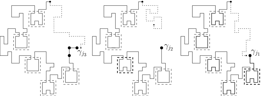
We will make some use of the notion of shell, but will predominantly consider a slightly different definition, the -local shell, which we now develop. This new notion concerns polygons rather than walks.
Recall that the parameter has been fixed in Subsection 4.1. (The upcoming definitions do not require that be fixed in this particular way in order to make sense, but, when we make use of the definitions, it will be for this choice of .) Define an equivalence relation on as follows. For any , let denote the polygon in the shell of that has no type patterns, (formed by switching every type pattern of into a type pattern). Thus, , where denotes the total number of type patterns in . A type pattern contains thirteen edges (in ; at least this number in higher dimensions), and these patterns are disjoint, so . Thus, the length of is at least . Let denote the set of slots in that are slots in , and, writing for the length of , let denote the set of slots in that are slots in . Note that and are disjoint. We further write and for the number of patterns of the given type in the slots , and and for the number of type patterns occupying slots in and in ; and similarly for and .
For , we say that if may be obtained from by relocating the type patterns of contained in the set of slots for to another set of locations among these slots. The relation is an equivalence relation, because the polygon formed by filling all the slots of with type patterns is shared by related polygons, so that the value of is equal for such polygons. Elements of a given equivalence class have common values of length, and , but not of or for . We call the equivalence classes -local shells: the parameter appears to denote the common length of the member polygons, and the term local is included to indicate that members of a given class may differ only in locations that are close to the origin (in the chemical distance, along the polygon). Complementing the notation for the shell of , write for the -local shell of .
For , write for the set of -local shells such that each of the quantities , , and is at least . Such “good” shells are highly typical if is small, as we now see.
Lemma 4.5.
There exist constants and such that
Proof. By Kesten’s pattern theorem [15, Theorem 1], there exist constants and such that, for any odd ,
| (4.3) |
where naturally denotes the number of type patterns in .
Note that every slot of is also a slot in : after all, the distance to be traversed to reach a given vertex in is at least as great along as it is along , because of the removal of type patterns by which is formed from . Thus,
Set
so that (4.3) implies . There exist constants such that
where the second inequality relies on both parts of Lemma 2.3, and the third entails a relabelling of . Thus, . The same holds for the quantity . Considering in place of , the same conclusion may be reached about and . It follows that
This completes the proof. ∎
In the next lemma, we see how, for any , the mixing of patterns that occurs when an element of is realized involves an asymptotically Gaussian fluctuation in the pattern number . The statement and proof are minor variations of those of [4, Lemma 3.5].
Lemma 4.6.
For any , there exists and such that, for and ,
(1) if satisfies , then
(2) and, for any ,
Proof. Fix a choice of in . If is distributed according to conditionally on , then type patterns and type patterns are distributed uniformly in the slots of . Thus, for ,
| (4.4) |
Write , and . By assumption and . Let . Under , is a random variable of mean , such that .
First, we investigate the case where is close to its mean. By means of a computation which uses Stirling’s formula and (4.4), we find that
| (4.5) |
where designates a quantity tending to as tends to infinity, uniformly in the acceptable choices of , , and , with . We have obtained Lemma 4.6(1).
We now turn to the deviations of from its mean. From (4.4), one can easily derive that is unimodal in with maximum at the value closest to that may take. (We remind the reader that takes values in , which contains only if .) The asymptotic equality (4.5) thus implies the existence of constants depending only on such that, for and large enough,
| (4.6) |
while for given , and large enough,
| (4.7) |
4.3. Mixing patterns by a random resampling
Consider a random resampling experiment whose law we will denote by . First an input polygon is sampled according to the law . Then the contents of the slots in are forgotten and independently resampled to form an output polygon . That is, given , is chosen uniformly among the set of polygons for which . Explicitly, if there are type patterns among slots in in (so that ), the polygon is formed by choosing uniformly at random a subset of cardinality of these slots and inserting type patterns into the chosen slots.
Note the crucial property that under has the law : the resampling experiment holds the length random polygon at equilibrium. We mention in passing that a basic consequence of this resampling is a delocalization of the walk midpoint.
Proposition 4.7.
[4, Proposition 1.3] Let . There exists such that, for ,
It may be instructive to consider how to proof this result using the resampling experiment (or in fact a similar one involving walks rather than polygons) and Lemma 4.5; a proof using such an approach is given in [4, Section 3.2].
Any element begins by tracing a journey over the region where slots in may appear, from the origin to ; it then follows its middle section, the trajectory of from until (where ); and it ends by moving from this vertex back to the origin, through the territory of slots in . Note that, in traversing the middle section, is exactly following a sub-walk of , because no pattern changes have been made to this part of . The timing of the middle section of this trajectory is advanced or retarded according to how many type patterns are placed in the slots in . Each extra such pattern retards the schedule by two units. When has the minimum possible number of type patterns in the slots of , the middle section is traversed by as early as possible, the journey taking place during . When has the maximum possible number of type patterns in the slots of , this traversal occurs as late as possible, during . Since and , necessarily lies in the middle section whenever . Since the snake method parameter has been set to belong to the interval , we see that always lies in the middle section whenever .
Taking and conditioning on , note that the mean number of type patterns that end up in the slots in under is given by , because this expression is the product of the number of type patterns that are redistributed and the proportion of the available slots that lie in .
Consider now a polygon that achieves as closely as possible the mean value for the number of type patterns among the slots in : that is, equals . As we have noted, is always reached during the middle section of ’s three-stage journey. Define the middle index so that . Note that, given and this value of , the value of this index is independent of the choice of .
4.4. Snakes of walks with high closing probability are typical
Recall that the index parameter (and also ) were fixed in Subsection 4.1. Moving towards the proof of Proposition 4.1, we take and define to be the set
Henceforth in this proof, charming will mean -charming. (The parity constraint that is even is applied above because the walks of length considered in the definition of charming at index must be of odd length if they are to close.)
We have seen that is visited by during its middle section, when it is traversing a subpath of unchanged by pattern mixing. For this reason, we may define a random variable under by setting .
We now state a key property of the resampling procedure.
Lemma 4.8.
The events and coincide.
Proof. Note that the shells of and coincide, because may be obtained from by modifying the -status of some of its slots (these being certain slots in ). Thus, Lemma 4.4 implies the statement. ∎
Lemma 4.9.
Proof. Choosing small enough and abbreviating , Lemma 4.6(1) implies that, for each and ,
Thus, again taking any ,
where the second inequality made use of Lemma 4.8.
Averaging over such , we find that
where denotes the expectation associated with the law .
Note that
where in the first inequality we use that under has the law , and then apply Lemma 4.5, to find that . The final inequality above used Lemma 4.2.
Thus,
We find that is at most
Applying Markov’s inequality yields Lemma 4.9. ∎
Proof of Proposition 4.1. Lemma 4.6(2) implies that
is at least . Note that the interval centred on considered here is shorter than its counterpart in the definition of for . Applying Lemmas 4.5 and 4.9, we find that
When the complementary event occurs, is charming for at least one-quarter of the indices in , so that is an element of . (We write one-quarter rather than one-half here, because one-half of such indices are inadmissible due to their having the wrong parity.) ∎
References
- [1] R. Bauerschmidt, D. Brydges, and G. Slade. Logarithmic correction for the susceptibility of the 4-dimensional weakly self-avoiding walk: a renormalisation group analysis. arXiv:1403.7422. Commun. Math. Phys., to appear, 2014.
- [2] R. Bauerschmidt, H. Duminil-Copin, J. Goodman, and G. Slade. Lectures on self-avoiding walks. In D. Ellwood, C. Newman, V. Sidoravicius, and W. Werner, editors, Lecture notes, in Probability and Statistical Physics in Two and More Dimensions. CMI/AMS – Clay Mathematics Institute Proceedings, 2011.
- [3] Mireille Bousquet-Mélou and Richard Brak. Exactly solved models. In Polygons, polyominoes and polycubes, volume 775 of Lecture Notes in Phys., pages 43–78. Springer, Dordrecht, 2009.
- [4] Hugo Duminil-Copin, Ioan Manolescu, Alexander Glazman, and Alan Hammond. On the probability that self-avoiding walks ends at a given point. arXiv:1305.1257. Ann. Probab., to appear, 2013.
- [5] B. Duplantier. Fractals in two dimensions and conformal invariance. Phys. D, 38(1-3):71–87, 1989. Fractals in physics (Vence, 1989).
- [6] B. Duplantier. Renormalization and conformal invariance for polymers. In Fundamental problems in statistical mechanics VII (Altenberg, 1989), pages 171–223. North-Holland, Amsterdam, 1990.
- [7] P. Flory. Principles of Polymer Chemistry. Cornell University Press, 1953.
- [8] J. M. Hammersley and D. J. A. Welsh. Further results on the rate of convergence to the connective constant of the hypercubical lattice. Quart. J. Math. Oxford Ser. (2), 13:108–110, 1962.
- [9] Alan Hammond. On self-avoiding polygons and walks: counting, joining and closing. arXiv:1504.05286, 2017.
- [10] Alan Hammond. On self-avoiding polygons and walks: the snake method via polygon joining. math.berkeley.edu/~alanmh/papers/snakemethodpolygon.pdf, 2017.
- [11] Alan Hammond. An upper bound on the number of self-avoiding polygons via joining. math.berkeley.edu/~alanmh/papers/ThetaBound.pdf, 2017.
- [12] T. Hara and G. Slade. Self-avoiding walk in five or more dimensions. I. The critical behaviour. Comm. Math. Phys., 147(1):101–136, 1992.
- [13] Takashi Hara and Gordon Slade. The lace expansion for self-avoiding walk in five or more dimensions. Rev. Math. Phys., 4(2):235–327, 1992.
- [14] E. J. Jance van Rensburg, E. Orlandini, D. W. Sumners, M. C. Tesi, and S. G. Whittington. The writhe of a self-avoiding polygon. Journal of Physics A: Mathematical and General, 26(19):L981 – L986, 1993.
- [15] H. Kesten. On the number of self-avoiding walks. J. Mathematical Phys., 4:960–969, 1963.
- [16] G. Lawler. Random walk problems motivated by statistical physics. http://www.math.uchicago.edu/ lawler/russia.pdf, 2013.
- [17] G. F. Lawler, O. Schramm, and W. Werner. On the scaling limit of planar self-avoiding walk. In Fractal geometry and applications: a jubilee of Benoît Mandelbrot, Part 2, volume 72 of Proc. Sympos. Pure Math., pages 339–364. Amer. Math. Soc., Providence, RI, 2004.
- [18] N. Madras. A lower bound for the end-to-end distance of the self-avoiding walk. Canad. Math. Bull., 57(1):113–118, 2014.
- [19] N. Madras and G. Slade. The self-avoiding walk. Probability and its Applications. Birkhäuser Boston Inc., Boston, MA, 1993.
- [20] B. Nienhuis. Exact critical point and critical exponents of models in two dimensions. Phys. Rev. Lett., 49:1062–1065, 1982.
- [21] B. Nienhuis. Coulomb gas description of 2D critical behaviour. J. Statist. Phys., 34:731–761, 1984.
- [22] W.J.C. Orr. Statistical treatment of polymer solutions at infinite dilution. Transactions of the Faraday Society, 43:12–27, 1947.