跳到论文正文
W Papers独立论文阅读器 arXiv:1808.09566 论文正文 计算阅读时间 · 0%
引用这篇论文根据当前论文元数据生成,正式投稿前建议核对。


License: arXiv.org perpetual non-exclusive license
arXiv:1808.09566v2 [math.OC] 18 Sep 2018

Privacy-preserving Decentralized Optimization via Decomposition

Chunlei Zhang    Huan Gao    Yongqiang Wang ††thanks: Chunlei Zhang, Huan Gao, and Yongqiang Wang are with the department of Electrical and Computer Engineering, Clemson University, Clemson, SC 29634, USA {chunlez, hgao2, yongqiw}@clemson.edu
Abstract

This paper considers the problem of privacy-preservation in decentralized optimization, in which NN agents cooperatively minimize a global objective function that is the sum of NN local objective functions. We assume that each local objective function is private and only known to an individual agent. To cooperatively solve the problem, most existing decentralized optimization approaches require participating agents to exchange and disclose estimates to neighboring agents. However, this results in leakage of private information about local objective functions, which is undesirable when adversaries exist and try to steal information from participating agents. To address this issue, we propose a privacy-preserving decentralized optimization approach based on proximal Jacobian ADMM via function decomposition. Numerical simulations confirm the effectiveness of the proposed approach.

I Introduction

We consider the problem of privacy-preservation in decentralized optimization where NN agents cooperatively minimize a global objective function of the following form:

min𝒙~f¯​(𝒙~)=∑i=1Nfi​(𝒙~),\displaystyle\mathop{\min}\limits_{\tilde{\bm{x}}}\qquad\bar{f}(\tilde{\bm{x}})=\sum\limits_{i=1}^{N}f_{i}(\tilde{\bm{x}}), (1)

where variable 𝒙~∈ℝn\tilde{\bm{x}}\in\mathbb{R}^{n} is common to all agents, function fi:ℝn→ℝf_{i}:\mathbb{R}^{n}\to\mathbb{R} is a private local objective function of agent ii. This problem has found wide applications in various domains, ranging from rendezvous in multi-agent systems [1], support vector machine [2] and classification [3] in machine learning, source localization in sensor networks [4], to data regression in statistics [5, 6].

To solve the optimization problem (1) in an decentralized manner, different algorithms were proposed in recent years, including the distributed (sub)gradient algorithm [7], augmented Lagrangian methods (ALM) [8], and the alternating direction method of multipliers (ADMM) as well as its variants [9, 8, 10, 11]. Among existing approaches, ADMM has attracted tremendous attention due to its wide applications [9] and fast convergence rate in both primal and dual iterations [11]. ADMM yields a convergence rate of O⁡(1/k)O(1/k) when the local objective functions fif_{i} are convex and a Q-linear convergence rate when all the local objective functions are strongly convex [12]. In addition, a recent work shows that ADMM can achieve a Q-linear convergence rate even when the local objective functions are only convex (subject to the constraint that the global objective function is strongly convex) [13].

On the other hand, privacy has become one of the key concerns. For example, in source localization, participating agents may want to reach consensus on the source position without revealing their position information [14]. In the rendezvous problem, a group of individuals may want to meet at an agreed time and place [1] without leaking their initial locations [15]. In the business sector, independent companies may want to work together to complete a common business for mutual benefit but without sharing their private data [16]. In the agreement problem [17], a group of organizations may want to reach consensus on a subject without leaking their individual opinions to others [15].

One widely used approach to enabling privacy-preservation in decentralized optimization is differential privacy [18, 19, 20, 21] which protects sensitive information by adding carefully-designed noise to exchanged states or objective functions. However, adding noise also compromises the accuracy of optimization results and causes a fundamental trade-off between privacy and accuracy [18, 19, 20]. In fact, approaches based on differential privacy may fail to converge to the accurate optimization result even without noise perturbation [20]. It is worth noting that there exists some differential-privacy based optimization approaches which are able to converge to the accurate optimization result in the mean-square sense, e.g. [22, 23]. However, those results require the assistance of a third party such as a cloud [22, 23], and therefore cannot be applied to the completely decentralized setting where no third parties exist. Encryption-based approaches are also commonly used to enable privacy-preservation [24, 25, 26]. However, such approaches unavoidably bring about extra computational and communication burden for real-time optimization [27]. Another approach to enabling privacy preservation in linear multi-agent networks is observability-based design [28, 29], which protects agents’ information from non-neighboring agents through properly designing the weights of the communication graph. However, this approach cannot protect the privacy of adversary’s direct neighbors.

To enable privacy in decentralized optimization without incurring large communication/computational overhead or compromising algorithmic accuracy, we propose a novel privacy solution through function decomposition. In the optimization literature, privacy has been defined as preserving the confidentiality of agents’ states [22], (sub)gradients or objective functions [20, 30, 31]. In this paper, we define privacy as the non-disclosure of agents’ (sub)gradients. We protect agents’ (sub)gradients because in many decentralized optimization applications, subgradients contain sensitive information such as salary or medical record [26, 30].

Contributions: We proposed a privacy-preserving decentralized optimization approach through function decomposition. In contrast to differential-privacy based approaches which use noise to cover sensitive information and are subject to a fundamental trade-off between privacy and accuracy, our approach can enable privacy preservation without sacrificing accuracy. Compared with encryption-based approaches which suffer from heavy computational and communication burden, our approach incurs little extra computational and communication overhead.

Organization: The rest of this paper is organized as follows: Sec. II introduces the attack model and presents the proximal Jacobian ADMM solution to (1). Then a completely decentralized privacy-preserving approach to problem (1) is proposed in Sec. III. Rigorous analysis of the guaranteed privacy and convergence is addressed in Sec. IV and Sec. V, respectively. Numerical simulation results are provided in Sec. VI to confirm the effectiveness and computational efficiency of the proposed approach. In the end, we draw conclusions in Sec. VII.

II Background

We first introduce the attack model considered in this paper. Then we present the proximal Jacobian ADMM algorithm for decentralized optimization.

II-A Attack Model

We consider two types of adversaries in this paper: Honest-but-curious adversaries and External eavesdroppers. Honest-but-curious adversaries are agents who follow all protocol steps correctly but are curious and collect all intermediate and input/output data in an attempt to learn some information about other participating agents [32]. External eavesdroppers are adversaries who steal information through wiretapping all communication channels and intercepting messages exchanged between agents.

II-B Proximal Jacobian ADMM

The decentralized problem (1) can be formulated as follows: each fif_{i} in (1) is private and only known to agent ii, and all NN agents form a bidirectional connected network, which is denoted by a graph G=(V,E)G=(V,E). VV denotes the set of agents, EE denotes the set of communication links (undirected edges) between agents, and |E||E| denotes the number of communication links (undirected edges) in EE. If there exists a communication link between agents ii and jj, we say that agent ii and agent jj are neighbors and the link is denoted as ei,j∈Ee_{i,j}\in E if i<ji<j is true or ej,i∈Ee_{j,i}\in E otherwise. Moreover, the set of all neighboring agents of ii is denoted as 𝒩i\mathcal{N}_{i} and the number of agents in 𝒩i\mathcal{N}_{i} is denoted as DiD_{i}. Then problem (1) can be rewritten as

min𝒙i∈ℝn,i∈{1,2,…,N}∑i=1Nfi​(𝒙i)\displaystyle\mathop{\min}\limits_{\bm{x}_{i}\in\mathbb{R}^{n},\,i\in\{1,2,\ldots,N\}}\qquad\sum\limits_{i=1}^{N}f_{i}(\bm{x}_{i}) (2)
subject to𝒙i=𝒙j,∀ei,j∈E,\displaystyle\textrm{subject to}\qquad\bm{x}_{i}=\bm{x}_{j},\quad\forall e_{i,j}\in E,

where 𝒙i\bm{x}_{i} is a copy of 𝒙~\tilde{\bm{x}} and belongs to agent ii. Using the following proximal Jacobian ADMM [33], an optimal solution to (1) can be achieved at each agent:

𝒙ik+1=argmin𝒙ifi(𝒙i)+γi​ρ2∥𝒙i−𝒙ik∥2\displaystyle\bm{x}_{i}^{k+1}=\underset{\bm{x}_{i}}{\operatorname{argmin}}f_{i}(\bm{x}_{i})+\frac{\gamma_{i}\rho}{2}\parallel\bm{x}_{i}-\bm{x}_{i}^{k}\parallel^{2}
+∑j∈𝒩i(𝝀i,jk​T(𝒙i−𝒙jk)+ρ2∥𝒙i−𝒙jk∥2),\displaystyle\qquad\qquad+\sum\limits_{j\in\mathcal{N}_{i}}(\bm{\lambda}_{i,j}^{kT}(\bm{x}_{i}-\bm{x}_{j}^{k})+\frac{\rho}{2}\parallel\bm{x}_{i}-\bm{x}_{j}^{k}\parallel^{2}), (3)
𝝀i,jk+1=𝝀i,jk+ρ⁡(𝒙ik+1−𝒙jk+1),∀j∈𝒩i.\displaystyle\bm{\lambda}_{i,j}^{k+1}=\bm{\lambda}_{i,j}^{k}+\rho(\bm{x}_{i}^{k+1}-\bm{x}_{j}^{k+1}),\quad\forall j\in\mathcal{N}_{i}. (4)

Here, kk is the iteration index, γi>0\gamma_{i}>0 (i=1,2,…,N)(i=1,2,\ldots,N) are proximal coefficients, ρ\rho is the penalty parameter, which is a positive constant scalar. 𝝀i,j\bm{\lambda}_{i,j} and 𝝀j,i\bm{\lambda}_{j,i} are Lagrange multipliers corresponding to the constraint 𝒙i=𝒙j,ei,j∈E\bm{x}_{i}=\bm{x}_{j},e_{i,j}\in E. It is worth noting that similar to our prior work [26], both 𝝀i,j\bm{\lambda}_{i,j} and 𝝀j,i\bm{\lambda}_{j,i} are introduced for the constraint 𝒙i=𝒙j,ei,j∈E\bm{x}_{i}=\bm{x}_{j},e_{i,j}\in E in (3)-(4) to unify the algorithm description. By setting 𝝀i,j0=ρ⁡(𝒙i0−𝒙j0)\bm{\lambda}_{i,j}^{0}=\rho(\bm{x}_{i}^{0}-\bm{x}_{j}^{0}) at t=0t=0, we have 𝝀i,jk=−𝝀j,ik\bm{\lambda}_{i,j}^{k}=-\bm{\lambda}_{j,i}^{k} holding for all i=1,2,⋯,N,j∈𝒩ii=1,2,\cdots,N,j\in\mathcal{N}_{i}. In this way, the update rule of agent ii can be unified without separating i>ji>j and i<ji<j for j∈𝒩ij\in\mathcal{N}_{i}, as shown in (3).

The proximal Jacobian ADMM is effective in solving (1). However, it cannot protect the privacy of participating agents’ gradients as states 𝒙ik\bm{x}_{i}^{k} are exchanged and disclosed explicitly among neighboring agents. So adversaries can easily derive ▽​fi​(𝒙ik)\triangledown f_{i}(\bm{x}_{i}^{k}) explicitly for k=1,2,…k=1,2,\ldots according to the update rules in (3) and (4) by leveraging the knowledge of γi\gamma_{i}.

III Privacy-preserving Decentralized Optimization

The key idea of our approach to enabling privacy-preservation is to randomly decompose each fif_{i} into two parts fiα​kf_{i}^{\alpha k} and fiβ​kf_{i}^{\beta k} under the constraint fi=fiα​k+fiβ​kf_{i}=f_{i}^{\alpha k}+f_{i}^{\beta k}. The index kk of functions fiα​kf_{i}^{\alpha k} and fiβ​kf_{i}^{\beta k} indicates that functions fiα​kf_{i}^{\alpha k} and fiβ​kf_{i}^{\beta k} can be time-varying. However, it should be noticed that the sum of fiα​kf_{i}^{\alpha k} and fiβ​kf_{i}^{\beta k} is time invariant and always equals to fif_{i}. We let the function fiα​kf_{i}^{\alpha k} succeed the role of the original function fif_{i} in inter-agent interactions while the other function fiβ​kf_{i}^{\beta k} involves only by interacting with fiα​kf_{i}^{\alpha k}, as shown in Fig. 1.

Refer to caption
(a)
Refer to caption
(b)
Fig. 1: Function-decomposition based privacy-preserving decentralized optimization. (a) Before function decomposition (b) after function decomposition.

After the function decomposition, problem (1) can be rewritten as

min𝒙iα,𝒙iβ∈ℝn,i∈{1,2,…,N}∑i=1N(fiα​k​(𝒙iα)+fiβ​k​(𝒙iβ))\displaystyle\mathop{\min}\limits_{\bm{x}_{i}^{\alpha},\bm{x}_{i}^{\beta}\in\mathbb{R}^{n},\,i\in\{1,2,\ldots,N\}}\qquad\sum\limits_{i=1}^{N}(f_{i}^{\alpha k}(\bm{x}_{i}^{\alpha})+f_{i}^{\beta k}(\bm{x}_{i}^{\beta})) (5)
subject to𝒙iα=𝒙jα,∀ei,j∈E,\displaystyle\textrm{subject to}\qquad\quad\bm{x}_{i}^{\alpha}=\bm{x}_{j}^{\alpha},\quad\forall e_{i,j}\in E,
𝒙iα=𝒙iβ,∀i∈V,\displaystyle\bm{x}_{i}^{\alpha}=\bm{x}_{i}^{\beta},\quad\forall i\in V,

and the associated augmented Lagrangian function is

ℒρk​(𝒙,𝝀)=∑i=1N(fiα​k​(𝒙iα)+fiβ​k​(𝒙iβ))\displaystyle\lx@add@cssclass{ltx_eqn_lefteqn}$\displaystyle\mathcal{L}_{\rho}^{k}(\bm{x},\bm{\lambda})=\sum\limits_{i=1}^{N}(f_{i}^{\alpha k}(\bm{x}_{i}^{\alpha})+f_{i}^{\beta k}(\bm{x}_{i}^{\beta}))$\mbox{} (6)
+∑ei,j∈E(𝝀i,jα​T(𝒙iα−𝒙jα)+ρ2∥𝒙iα−𝒙jα∥2)\displaystyle+\sum\limits_{e_{i,j}\in E}(\bm{\lambda}_{i,j}^{\alpha T}(\bm{x}_{i}^{\alpha}-\bm{x}_{j}^{\alpha})+\frac{\rho}{2}\parallel\bm{x}_{i}^{\alpha}-\bm{x}_{j}^{\alpha}\parallel^{2})
+∑i∈V(𝝀i,iα​β​T(𝒙iα−𝒙iβ)+ρ2∥𝒙iα−𝒙iβ∥2).\displaystyle+\sum\limits_{i\in V}(\bm{\lambda}_{i,i}^{\alpha\beta T}(\bm{x}_{i}^{\alpha}-\bm{x}_{i}^{\beta})+\frac{\rho}{2}\parallel\bm{x}_{i}^{\alpha}-\bm{x}_{i}^{\beta}\parallel^{2}).

where 𝒙=[𝒙1α​T,𝒙1β​T,𝒙2α​T,𝒙2β​T,…,𝒙Nα​T,𝒙Nβ​T]T∈ℝ2​N​n\bm{x}=[\bm{x}_{1}^{\alpha T},\bm{x}_{1}^{\beta T},\bm{x}_{2}^{\alpha T},\bm{x}_{2}^{\beta T},\ldots,\bm{x}_{N}^{\alpha T},\bm{x}_{N}^{\beta T}]^{T}\in\mathbb{R}^{2Nn} is the augmented state. 𝝀i,jα\bm{\lambda}_{i,j}^{\alpha} is the Lagrange multiplier corresponding to the constraint 𝒙iα=𝒙jα\bm{x}_{i}^{\alpha}=\bm{x}_{j}^{\alpha}, 𝝀i,iα​β\bm{\lambda}_{i,i}^{\alpha\beta} is the Lagrange multiplier corresponding to the constraint 𝒙iα=𝒙iβ\bm{x}_{i}^{\alpha}=\bm{x}_{i}^{\beta}, and all 𝝀i,jα\bm{\lambda}_{i,j}^{\alpha} and 𝝀i,iα​β\bm{\lambda}_{i,i}^{\alpha\beta} are stacked into 𝝀\bm{\lambda}. ρ\rho is the penalty parameter, which is a positive constant scalar. It is worth noting that each agent ii does not need to know the associated augmented Lagrangian function (i.e., other agents’ objective functions) to update its states 𝒙iα\bm{x}_{i}^{\alpha} and 𝒙iβ\bm{x}_{i}^{\beta}, as shown below in (7) and (8).

Based on Jacobian update, we can solve (5) by applying the following iterations for i=1,2,…,Ni=1,2,\ldots,N:

𝒙iα⁡(k+1)=argmin𝒙iαγiα​ρ2∥𝒙iα−𝒙iα​k∥2\displaystyle\bm{x}_{i}^{\alpha(k+1)}=\underset{\bm{x}_{i}^{\alpha}}{\operatorname{argmin}}\frac{\gamma_{i}^{\alpha}\rho}{2}\parallel\bm{x}_{i}^{\alpha}-\bm{x}_{i}^{\alpha k}\parallel^{2}
+ℒρk+1​(𝒙1α​k,𝒙1β​k,…,𝒙iα,𝒙iβ​k,…,𝒙Nα​k,𝒙Nβ​k,𝝀k)\displaystyle\qquad\qquad+\mathcal{L}_{\rho}^{k+1}(\bm{x}_{1}^{\alpha k},\bm{x}_{1}^{\beta k},\ldots,\bm{x}_{i}^{\alpha},\bm{x}_{i}^{\beta k},\ldots,\bm{x}_{N}^{\alpha k},\bm{x}_{N}^{\beta k},\bm{\lambda}^{k})
=argmin𝒙iαfiα⁡(k+1)(𝒙iα)+γiα​ρ2∥𝒙iα−𝒙iα​k∥2\displaystyle\qquad\qquad=\underset{\bm{x}_{i}^{\alpha}}{\operatorname{argmin}}f_{i}^{\alpha(k+1)}(\bm{x}_{i}^{\alpha})+\frac{\gamma_{i}^{\alpha}\rho}{2}\parallel\bm{x}_{i}^{\alpha}-\bm{x}_{i}^{\alpha k}\parallel^{2}
+∑j∈𝒩i(𝝀i,jα​k​T(𝒙iα−𝒙jα​k)+ρ2∥𝒙iα−𝒙jα​k∥2)\displaystyle\qquad\qquad+\sum\limits_{j\in\mathcal{N}_{i}}(\bm{\lambda}_{i,j}^{\alpha kT}(\bm{x}_{i}^{\alpha}-\bm{x}_{j}^{\alpha k})+\frac{\rho}{2}\parallel\bm{x}_{i}^{\alpha}-\bm{x}_{j}^{\alpha k}\parallel^{2})
+𝝀i,iα​β​k​T(𝒙iα−𝒙iβ​k)+ρ2∥𝒙iα−𝒙iβ​k∥2,\displaystyle\qquad\qquad+\bm{\lambda}_{i,i}^{\alpha\beta kT}(\bm{x}_{i}^{\alpha}-\bm{x}_{i}^{\beta k})+\frac{\rho}{2}\parallel\bm{x}_{i}^{\alpha}-\bm{x}_{i}^{\beta k}\parallel^{2}, (7)
𝒙iβ⁡(k+1)=argmin𝒙iβγiβ​ρ2∥𝒙iβ−𝒙iβ​k∥2\displaystyle\bm{x}_{i}^{\beta(k+1)}=\underset{\bm{x}_{i}^{\beta}}{\operatorname{argmin}}\frac{\gamma_{i}^{\beta}\rho}{2}\parallel\bm{x}_{i}^{\beta}-\bm{x}_{i}^{\beta k}\parallel^{2}
+ℒρk+1​(𝒙1α​k,𝒙1β​k,…,𝒙iα​k,𝒙iβ,…,𝒙Nα​k,𝒙Nβ​k,𝝀k)\displaystyle\qquad\qquad+\mathcal{L}_{\rho}^{k+1}(\bm{x}_{1}^{\alpha k},\bm{x}_{1}^{\beta k},\ldots,\bm{x}_{i}^{\alpha k},\bm{x}_{i}^{\beta},\ldots,\bm{x}_{N}^{\alpha k},\bm{x}_{N}^{\beta k},\bm{\lambda}^{k})
=argmin𝒙iβfiβ⁡(k+1)(𝒙iβ)+γiβ​ρ2∥𝒙iβ−𝒙iβ​k∥2\displaystyle\qquad\qquad=\underset{\bm{x}_{i}^{\beta}}{\operatorname{argmin}}f_{i}^{\beta(k+1)}(\bm{x}_{i}^{\beta})+\frac{\gamma_{i}^{\beta}\rho}{2}\parallel\bm{x}_{i}^{\beta}-\bm{x}_{i}^{\beta k}\parallel^{2}
+𝝀i,iβ​α​k​T(𝒙iβ−𝒙iα​k)+ρ2∥𝒙iβ−𝒙iα​k∥2,\displaystyle\qquad\qquad+\bm{\lambda}_{i,i}^{\beta\alpha kT}(\bm{x}_{i}^{\beta}-\bm{x}_{i}^{\alpha k})+\frac{\rho}{2}\parallel\bm{x}_{i}^{\beta}-\bm{x}_{i}^{\alpha k}\parallel^{2}, (8)
𝝀i,jα⁡(k+1)=𝝀i,jα​k+ρ⁡(𝒙iα⁡(k+1)−𝒙jα⁡(k+1)),∀j∈𝒩i\displaystyle\bm{\lambda}_{i,j}^{\alpha(k+1)}=\bm{\lambda}_{i,j}^{\alpha k}+\rho(\bm{x}_{i}^{\alpha(k+1)}-\bm{x}_{j}^{\alpha(k+1)}),\quad\forall j\in\mathcal{N}_{i} (9)
𝝀i,iα​β​(k+1)=𝝀i,iα​β​k+ρ⁡(𝒙iα⁡(k+1)−𝒙iβ⁡(k+1)),\displaystyle\bm{\lambda}_{i,i}^{\alpha\beta(k+1)}=\bm{\lambda}_{i,i}^{\alpha\beta k}+\rho(\bm{x}_{i}^{\alpha(k+1)}-\bm{x}_{i}^{\beta(k+1)}), (10)
𝝀i,iβ​α​(k+1)=𝝀i,iβ​α​k+ρ⁡(𝒙iβ⁡(k+1)−𝒙iα⁡(k+1)).\displaystyle\bm{\lambda}_{i,i}^{\beta\alpha(k+1)}=\bm{\lambda}_{i,i}^{\beta\alpha k}+\rho(\bm{x}_{i}^{\beta(k+1)}-\bm{x}_{i}^{\alpha(k+1)}). (11)

Here, similar to our prior work [26] and algorithm (3)-(4), both 𝝀i,jα\bm{\lambda}_{i,j}^{\alpha} and 𝝀j,iα\bm{\lambda}_{j,i}^{\alpha} are introduced for the constraint 𝒙iα=𝒙jα,ei,j∈E\bm{x}_{i}^{\alpha}=\bm{x}_{j}^{\alpha},e_{i,j}\in E in (7)-(11) to unify the algorithm description. Similarly, both 𝝀i,iα​β\bm{\lambda}_{i,i}^{\alpha\beta} and 𝝀i,iβ​α\bm{\lambda}_{i,i}^{\beta\alpha} are introduced for the constraint 𝒙iα=𝒙iβ\bm{x}_{i}^{\alpha}=\bm{x}_{i}^{\beta} in (7)-(11) to unify the algorithm description.

Next we give in detail our privacy-preserving function-decomposition based algorithm.


Algorithm I


Initial Setup: For all i=1,2,…,Ni=1,2,\ldots,N, agent ii initializes 𝒙iα​0\bm{x}_{i}^{\alpha 0} and 𝒙iβ​0\bm{x}_{i}^{\beta 0}, and exchanges 𝒙iα​0\bm{x}_{i}^{\alpha 0} with neighboring agents. Then agent ii sets 𝝀i,jα​0=𝒙iα​0−𝒙jα​0\bm{\lambda}_{i,j}^{\alpha 0}=\bm{x}_{i}^{\alpha 0}-\bm{x}_{j}^{\alpha 0}, 𝝀i,iα​β​0=𝒙iα​0−𝒙iβ​0\bm{\lambda}_{i,i}^{\alpha\beta 0}=\bm{x}_{i}^{\alpha 0}-\bm{x}_{i}^{\beta 0}, and 𝝀i,iβ​α​0=𝒙iβ​0−𝒙iα​0\bm{\lambda}_{i,i}^{\beta\alpha 0}=\bm{x}_{i}^{\beta 0}-\bm{x}_{i}^{\alpha 0}.

Input: 𝒙iα​k\bm{x}_{i}^{\alpha k}, 𝝀i,jα​k\bm{\lambda}_{i,j}^{\alpha k}, 𝝀i,iα​β​k\bm{\lambda}_{i,i}^{\alpha\beta k}, 𝒙iβ​k\bm{x}_{i}^{\beta k}, 𝝀i,iβ​α​k\bm{\lambda}_{i,i}^{\beta\alpha k}.

Output: 𝒙iα⁡(k+1)\bm{x}_{i}^{\alpha(k+1)}, 𝝀i,jα⁡(k+1)\bm{\lambda}_{i,j}^{\alpha(k+1)}, 𝝀i,iα​β​(k+1)\bm{\lambda}_{i,i}^{\alpha\beta(k+1)}, 𝒙iβ⁡(k+1)\bm{x}_{i}^{\beta(k+1)}, 𝝀i,iβ​α​(k+1)\bm{\lambda}_{i,i}^{\beta\alpha(k+1)}.

  1. 1.

    For all i=1,2,…,Ni=1,2,\ldots,N, agent ii constructs fiα⁡(k+1)f_{i}^{\alpha(k+1)} and fiβ⁡(k+1)f_{i}^{\beta(k+1)} under the constraint fi=fiα⁡(k+1)+fiβ⁡(k+1)f_{i}=f_{i}^{\alpha(k+1)}+f_{i}^{\beta(k+1)};

  2. 2.

    For all i=1,2,…,Ni=1,2,\ldots,N, agent ii updates 𝒙iα⁡(k+1)\bm{x}_{i}^{\alpha(k+1)} and 𝒙iβ⁡(k+1)\bm{x}_{i}^{\beta(k+1)} according to the update rules in (7) and (8), respectively;

  3. 3.

    For all i=1,2,…,Ni=1,2,\ldots,N, agent ii sends 𝒙iα⁡(k+1)\bm{x}_{i}^{\alpha(k+1)} to neighboring agents;

  4. 4.

    For all i=1,2,…,Ni=1,2,\ldots,N, agent ii computes 𝝀i,jα⁡(k+1)\bm{\lambda}_{i,j}^{\alpha(k+1)}, 𝝀i,iα​β​(k+1)\bm{\lambda}_{i,i}^{\alpha\beta(k+1)} and 𝝀i,iβ​α​(k+1)\bm{\lambda}_{i,i}^{\beta\alpha(k+1)} according to (9)-(11);

  5. 5.

    Set kk to k+1k+1, and go to 1).


IV Privacy Analysis

In this section, we rigorously prove that each agent’s gradient of local objective function ▽​fj\triangledown f_{j} cannot be inferred by honest-but-curious adversaries and external eavesdroppers.

Theorem 1

In Algorithm I, agent jj’s gradient of local objective function ▽​fj\triangledown f_{j} at any point except the optimal solution will not be revealed to an honest-but-curious agent ii.

Proof:

Suppose that an honest-but-curious adversary agent ii collects information from KK iterations to infer the gradient ▽​fj\triangledown f_{j} of a neighboring agent jj. The adversary agent ii can establish 2​n​K2nK equations relevant to ▽​fj\triangledown f_{j} by making use of the fact that the update rules of (7) and (8) are publicly known, i.e.,

{▽​fjα​1​(𝒙jα​1)+(γjα+Dj+1)​ρ​𝒙jα​1−γjα​ρ​𝒙jα​0+∑m∈𝒩j(𝝀j,mα​0−ρ𝒙mα​0)+𝝀j,jα​β​0−ρ𝒙jβ​0=𝟎,▽​fjβ​1​(𝒙jβ​1)+(γjβ+1)​ρ​𝒙jβ​1−γjβ​ρ​𝒙jβ​0+𝝀j,jβ​α​0−ρ​𝒙jα​0=𝟎,⋮▽​fjα​K​(𝒙jα​K)+(γjα+Dj+1)​ρ​𝒙jα​K−γjα​ρ​𝒙jα⁡(K−1)+∑m∈𝒩j(𝝀j,mα⁡(K−1)−ρ​𝒙mα⁡(K−1))+𝝀j,jα​β​(K−1)−ρ​𝒙jβ⁡(K−1)=𝟎,▽​fjβ​K​(𝒙jβ​K)+(γjβ+1)​ρ​𝒙jβ​K−γjβ​ρ​𝒙jβ⁡(K−1)+𝝀j,jβ​α​(K−1)−ρ​𝒙jα⁡(K−1)=𝟎.\left\{\begin{aligned} \lx@add@cssclass{ltx_eqn_lefteqn}$\displaystyle\triangledown f_{j}^{\alpha 1}(\bm{x}_{j}^{\alpha 1})+(\gamma_{j}^{\alpha}+D_{j}+1)\rho\bm{x}_{j}^{\alpha 1}-\gamma_{j}^{\alpha}\rho\bm{x}_{j}^{\alpha 0}$\mbox{}\hfil\\ &\qquad\qquad\quad+\sum\limits_{m\in\mathcal{N}_{j}}(\bm{\lambda}_{j,m}^{\alpha 0}-\rho\bm{x}_{m}^{\alpha 0})+\bm{\lambda}_{j,j}^{\alpha\beta 0}-\rho\bm{x}_{j}^{\beta 0}=\bm{0},\\ \lx@add@cssclass{ltx_eqn_lefteqn}$\displaystyle\triangledown f_{j}^{\beta 1}(\bm{x}_{j}^{\beta 1})+(\gamma_{j}^{\beta}+1)\rho\bm{x}_{j}^{\beta 1}-\gamma_{j}^{\beta}\rho\bm{x}_{j}^{\beta 0}+\bm{\lambda}_{j,j}^{\beta\alpha 0}-\rho\bm{x}_{j}^{\alpha 0}=\bm{0},$\mbox{}\hfil\\ &\qquad\qquad\qquad\qquad\vdots\\ \lx@add@cssclass{ltx_eqn_lefteqn}$\displaystyle\triangledown f_{j}^{\alpha K}(\bm{x}_{j}^{\alpha K})+(\gamma_{j}^{\alpha}+D_{j}+1)\rho\bm{x}_{j}^{\alpha K}-\gamma_{j}^{\alpha}\rho\bm{x}_{j}^{\alpha(K-1)}+$\mbox{}\hfil\\ &\sum\limits_{m\in\mathcal{N}_{j}}(\bm{\lambda}_{j,m}^{\alpha(K-1)}-\rho\bm{x}_{m}^{\alpha(K-1)})+\bm{\lambda}_{j,j}^{\alpha\beta(K-1)}-\rho\bm{x}_{j}^{\beta(K-1)}=\bm{0},\\ \lx@add@cssclass{ltx_eqn_lefteqn}$\displaystyle\triangledown f_{j}^{\beta K}(\bm{x}_{j}^{\beta K})+(\gamma_{j}^{\beta}+1)\rho\bm{x}_{j}^{\beta K}-\gamma_{j}^{\beta}\rho\bm{x}_{j}^{\beta(K-1)}$\mbox{}\hfil\\ &\qquad\qquad\qquad\qquad\qquad\quad+\bm{\lambda}_{j,j}^{\beta\alpha(K-1)}-\rho\bm{x}_{j}^{\alpha(K-1)}=\bm{0}.\\ \end{aligned}\right. (12)

In the system of 2​n​K2nK equations (12), ▽​fjα​k​(𝒙jα​k)\triangledown f_{j}^{\alpha k}(\bm{x}_{j}^{\alpha k}) (k=1,2,…,K)(k=1,2,\ldots,K), ▽​fjβ​k​(𝒙jβ​k)\triangledown f_{j}^{\beta k}(\bm{x}_{j}^{\beta k}) (k=1,2,…,K)(k=1,2,\ldots,K), γjα\gamma_{j}^{\alpha}, γjβ\gamma_{j}^{\beta}, and 𝒙jβ​k\bm{x}_{j}^{\beta k} (k=0,1,2,…,K)(k=0,1,2,\ldots,K) are unknown to adversary agent ii. Parameters 𝒙mα​k,m≠j\bm{x}_{m}^{\alpha k},m\neq j and 𝝀j,mα​k,m≠j\bm{\lambda}_{j,m}^{\alpha k},m\neq j are known to adversary agent ii only when agent mm and agent ii are neighbors. So the above system of 2​n​K2nK equations contains at least 3​n​K+n+23nK+n+2 unknown variables, and adversary agent ii cannot infer the gradient of local objective function ▽​fj\triangledown f_{j} by solving (12).

It is worth noting that after the optimization algorithm converges, adversary agent ii can have another piece of information according to the KKT conditions [33]:

▽fj(𝒙j∗)=−∑m∈𝒩j𝝀j,mα∗.\displaystyle\triangledown f_{j}(\bm{x}_{j}^{*})=-\sum_{m\in\mathcal{N}_{j}}\bm{\lambda}_{j,m}^{\alpha*}. (13)

If agent jj’s neighbors are also neighbors to agent ii, the exact gradient of fjf_{j} at the optimal solution can be inferred by an honest-but-curious agent ii. Therefore, agent jj’s gradient of local objective function ▽​fj\triangledown f_{j} will not be revealed to an honest-but-curious agent ii at any point except the optimal solution. ∎

Corollary 1

In Algorithm I, agent jj’s gradient of local objective function ▽​fj\triangledown f_{j} at any point except the optimal solution will not be revealed to external eavesdroppers.

Proof:

The proof can be obtained following a similar line of reasoning of Theorem 1. External eavesdroppers can also establish a system of 2​n​K2nK equations (12) to infer agent jj’s gradient ▽​fj\triangledown f_{j}. However, the number of unknowns ▽​fjα​k​(𝒙jα​k)\triangledown f_{j}^{\alpha k}(\bm{x}_{j}^{\alpha k}) (k=1,2,…,K)(k=1,2,\ldots,K), ▽​fjβ​k​(𝒙jβ​k)\triangledown f_{j}^{\beta k}(\bm{x}_{j}^{\beta k}) (k=1,2,…,K)(k=1,2,\ldots,K), γjα\gamma_{j}^{\alpha}, γjβ\gamma_{j}^{\beta}, and 𝒙jβ​k\bm{x}_{j}^{\beta k} (k=0,1,2,…,K)(k=0,1,2,\ldots,K) adds up to 3​n​k+n+23nk+n+2, making the system of equations established by the external eavesdropper undetermined. Therefore, external eavesdroppers cannot infer the gradient of local objective function ▽​fj\triangledown f_{j} at any point except the optimal solution. ∎

Remark 1

It is worth noting that if multiple adversary agents cooperate to infer the information of agent jj, they can only establish a system of 2​n​K2nK equations containing at least 3​n​K+n+23nK+n+2 unknown variables as well. Therefore, our algorithm can protect the privacy of agents against multiple honest-but-curious adversaries and external eavesdroppers.

V Convergence Analysis

In this section, we rigorously prove the convergence of Algorithm I under the following assumptions:

Assumption 1

Each local function fi:ℝn→ℝf_{i}:\mathbb{R}^{n}\to\mathbb{R} is strongly convex and continuously differentiable, i.e.,

(▽fi(𝒙~)−▽fi(𝒚~))T(𝒙~−𝒚~)≥mi∥𝒙~−𝒚~∥2.(\triangledown f_{i}(\tilde{\bm{x}})-\triangledown f_{i}(\tilde{\bm{y}}))^{T}(\tilde{\bm{x}}-\tilde{\bm{y}})\geq m_{i}\parallel\tilde{\bm{x}}-\tilde{\bm{y}}\parallel^{2}.

In addition, there exists a lower bound mf>0m_{f}>0 such that mi≥2​mf,∀i={1,2,…,N}m_{i}\geq 2m_{f},\forall i=\{1,2,\ldots,N\} is true.

Assumption 2

Each private local function fi:ℝn→ℝf_{i}:\mathbb{R}^{n}\to\mathbb{R} has Lipschitz continuous gradients, i.e.,

∥▽fi(𝒙~)−▽fi(𝒚~)∥≤Li∥𝒙~−𝒚~∥.\parallel\triangledown f_{i}(\tilde{\bm{x}})-\triangledown f_{i}(\tilde{\bm{y}})\parallel\leq L_{i}\parallel\tilde{\bm{x}}-\tilde{\bm{y}}\parallel.
Assumption 3

fiα​kf_{i}^{\alpha k} is chosen under the following conditions:

1) fiα​kf_{i}^{\alpha k} is strongly convex and differentiable, i.e.,

(▽fiα​k(𝒙~)−▽fiα​k(𝒚~))T(𝒙~−𝒚~)≥mf∥𝒙~−𝒚~∥2.(\triangledown f_{i}^{\alpha k}(\tilde{\bm{x}})-\triangledown f_{i}^{\alpha k}(\tilde{\bm{y}}))^{T}(\tilde{\bm{x}}-\tilde{\bm{y}})\geq m_{f}\parallel\tilde{\bm{x}}-\tilde{\bm{y}}\parallel^{2}.

2) fiβ​k=fi−fiα​kf_{i}^{\beta k}=f_{i}-f_{i}^{\alpha k} is strongly convex and differentiable, i.e.,

(▽fiβ​k(𝒙~)−▽fiβ​k(𝒚~))T(𝒙~−𝒚~)≥mf∥𝒙~−𝒚~∥2.(\triangledown f_{i}^{\beta k}(\tilde{\bm{x}})-\triangledown f_{i}^{\beta k}(\tilde{\bm{y}}))^{T}(\tilde{\bm{x}}-\tilde{\bm{y}})\geq m_{f}\parallel\tilde{\bm{x}}-\tilde{\bm{y}}\parallel^{2}.

3) fiα​kf_{i}^{\alpha k} has Lipschitz continuous gradients, i.e., there exists an L<+∞L<+\infty such that

∥▽fiα​k(𝒙~)−▽fiα​k(𝒚~)∥≤L∥𝒙~−𝒚~∥.\parallel\triangledown f_{i}^{\alpha k}(\tilde{\bm{x}})-\triangledown f_{i}^{\alpha k}(\tilde{\bm{y}})\parallel\leq L\parallel\tilde{\bm{x}}-\tilde{\bm{y}}\parallel.

4) fiβ​k=fi−fiα​kf_{i}^{\beta k}=f_{i}-f_{i}^{\alpha k} has Lipschitz continuous gradients, i.e., there exists an L<+∞L<+\infty such that

∥▽fiβ​k(𝒙~)−▽fiβ​k(𝒚~)∥≤L∥𝒙~−𝒚~∥.\parallel\triangledown f_{i}^{\beta k}(\tilde{\bm{x}})-\triangledown f_{i}^{\beta k}(\tilde{\bm{y}})\parallel\leq L\parallel\tilde{\bm{x}}-\tilde{\bm{y}}\parallel.

5) limk→∞fiα​k→fiα∗\lim\limits_{k\to\infty}f_{i}^{\alpha k}\to f_{i}^{\alpha*} and fiα​k​(𝐱~)f_{i}^{\alpha k}(\tilde{\bm{x}}) is bounded when 𝐱~\tilde{\bm{x}} is bounded.

It is worth noting that under Assumption 1 and Assumption 2, fiα​kf_{i}^{\alpha k} can be easily designed to meet Assumption 3. A quick example is fiα​k​(𝒙~)=mf2​𝒙~T​𝒙~+𝒃ik​T​𝒙~f_{i}^{\alpha k}(\tilde{\bm{x}})=\frac{m_{f}}{2}\tilde{\bm{x}}^{T}\tilde{\bm{x}}+\bm{b}_{i}^{kT}\tilde{\bm{x}} where 𝒃ik∈ℝn\bm{b}_{i}^{k}\in\mathbb{R}^{n} can be time-varying, and satisfies limk→∞𝒃ik→𝒃i∗\lim\limits_{k\to\infty}\bm{b}_{i}^{k}\to\bm{b}_{i}^{*} and −∞<|𝒃ik|<∞-\infty<\parallel\bm{b}_{i}^{k}\parallel<\infty.

Because the function decomposition process amounts to converting the original network to a virtual network G′=(V′,E′)G^{\prime}=(V^{\prime},E^{\prime}) of 2​N2N agents, as shown in Fig. 2, we analyze the convergence of our algorithm based on the virtual network G′=(V′,E′)G^{\prime}=(V^{\prime},E^{\prime}). To simplify and unify the notations, we relabel the local objective functions fiα​kf_{i}^{\alpha k} and fiβ​kf_{i}^{\beta k} for all i=1,2,…,Ni=1,2,\ldots,N as h1k,h2k,…,h2​Nkh_{1}^{k},h_{2}^{k},\dots,h_{2N}^{k}. We relabel the associated states 𝒙iα​k\bm{x}_{i}^{\alpha k} and 𝒙iβ​k\bm{x}_{i}^{\beta k} for all i=1,2,…,Ni=1,2,\dots,N as 𝒙1k,𝒙2k,…,𝒙2​Nk\bm{x}_{1}^{k},\bm{x}_{2}^{k},\dots,\bm{x}_{2N}^{k}. In addition, we relabel parameters γiα\gamma_{i}^{\alpha} and γiβ\gamma_{i}^{\beta} for all i=1,2,…,Ni=1,2,\dots,N correspondingly as γ1,γ2,…,γ2​N\gamma_{1},\gamma_{2},\ldots,\gamma_{2N}. Then problem (5) can be rewritten as

Refer to caption
(a) G=(V,E)G=(V,E) of NN agents
Refer to caption
(b) Virtual network G′=(V′,E′)G^{\prime}=(V^{\prime},E^{\prime}) of 2​N2N agents
Fig. 2: Function-decomposition based privacy-preserving decentralized optimization equals to converting the original network into a virtual network G′=(V′,E′)G^{\prime}=(V^{\prime},E^{\prime}) of 2​N2N agents.
min𝒙i∈ℝn,i∈{1,2,…,2​N}∑i=12​Nhik​(𝒙i)\displaystyle\mathop{\min}\limits_{\bm{x}_{i}\in\mathbb{R}^{n},\,i\in\{1,2,\ldots,2N\}}\qquad\sum\limits_{i=1}^{2N}h_{i}^{k}(\bm{x}_{i}) (14)
subject toA​𝒙=𝟎\displaystyle\textrm{subject to}\qquad\qquad A\bm{x}=\bm{0}

where 𝒙=[𝒙1T,𝒙2T,…,𝒙2​NT]T∈ℝ2​N​n\bm{x}=[\bm{x}_{1}^{T},\bm{x}_{2}^{T},\ldots,\bm{x}_{2N}^{T}]^{T}\in\mathbb{R}^{2Nn} and A=[am,l]⊗In∈ℝ|E′|​n×2​N​nA=[a_{m,l}]\otimes I_{n}\in\mathbb{R}^{|E^{\prime}|n\times 2Nn} is the edge-node incidence matrix of graph 𝒢′\mathcal{G}^{\prime} as defined in [34]. Parameter am,la_{m,l} is defined as

am,l={1if the ​mt​h​ edge originates from agent ​l,−1if the ​mt​h​ edge terminates at agent ​l,0otherwise.\displaystyle a_{m,l}=\left\{\begin{matrix}1&\textrm{if the }m^{th}\textrm{ edge originates from agent }l,\\ -1&\textrm{if the }m^{th}\textrm{ edge terminates at agent }l,\\ 0&\textrm{otherwise}.\end{matrix}\right.

We define each edge ei,je_{i,j} originating from ii and terminating at jj and denote an edge as ei,j∈E′e_{i,j}\in E^{\prime} if i<ji<j is true or ej,i∈E′e_{j,i}\in E^{\prime} otherwise.

Denote the iterating results in the kkth step in Algorithm I as follows:

𝒙k=[𝒙1k​T,𝒙2k​T,…,𝒙2​Nk​T]T∈ℝ2​N​n,\displaystyle\bm{x}^{k}=[\bm{x}_{1}^{kT},\bm{x}_{2}^{kT},\ldots,\bm{x}_{2N}^{kT}]^{T}\in\mathbb{R}^{2Nn},
𝝀k=[𝝀i,jk]i​j,ei,j∈E′∈ℝ|E′|​n,\displaystyle\bm{\lambda}^{k}=[\bm{\lambda}_{i,j}^{k}]_{ij,e_{i,j}\in E^{\prime}}\in\mathbb{R}^{|E^{\prime}|n},
𝒚k=[𝒙k​T,𝝀k​T]T∈ℝ(|E′|+2​N)​n\displaystyle\bm{y}^{k}=[\bm{x}^{kT},\bm{\lambda}^{kT}]^{T}\in\mathbb{R}^{(|E^{\prime}|+2N)n}

Further augment the coefficients γi\gamma_{i} (i=1,2,…,2​N)(i=1,2,\ldots,2N) into the matrix form

U=diag⁡{γ1,γ2,…,γ2​N}⊗In∈ℝ2​N​n×2​N​n,U={\rm diag}\{\gamma_{1},\gamma_{2},\ldots,\gamma_{2N}\}\otimes I_{n}\in\mathbb{R}^{2Nn\times 2Nn},

and DiD_{i} into the matrix form

D=diag⁡{D1,D2,…,D2​N}⊗In∈ℝ2​N​n×2​N​n.D={\rm diag}\{D_{1},D_{2},\ldots,D_{2N}\}\otimes I_{n}\in\mathbb{R}^{2Nn\times 2Nn}.

Now we are in position to give the main results for this section:

Lemma 1

Let 𝐱∗\bm{x}^{*} be the optimal solution, 𝛌k∗\bm{\lambda}^{k*} be the optimal multiplier to (14) at iteration kk, and 𝐲k∗=[𝐱∗T,𝛌k∗T]T\bm{y}^{k*}=[\bm{x}^{*T},\bm{\lambda}^{k*T}]^{T}. Further define Q=U+D−AT​AQ=U+D-A^{T}A, H=diag⁡{ρ​Q,1ρ​I|E′|​n}H={\rm diag}\{\rho Q,\frac{1}{\rho}I_{|E^{\prime}|n}\}, and let u>1u>1 be an arbitrary constant, then we have

∥𝒚k+1−𝒚k+1∗∥H≤∥𝒚k−𝒚k+1∗∥H1+δ\displaystyle\parallel\bm{y}^{k+1}-\bm{y}^{k+1*}\parallel_{H}\leq\frac{\parallel\bm{y}^{k}-\bm{y}^{k+1*}\parallel_{H}}{\sqrt{1+\delta}} (15)

if U+D−AT​AU+D-A^{T}A is positive semi-definite and Assumptions 1, 2, and 3 are satisfied. In (15), ∥𝐱~∥H=𝐱~T​H​𝐱~\parallel\tilde{\bm{x}}\parallel_{H}=\sqrt{\tilde{\bm{x}}^{T}H\tilde{\bm{x}}} and

δ=min⁡{(u−1)​Aminu​Qmax,2​mf​Amin​ρu​L2+ρ2​Amin​Qmax},\displaystyle\delta=\min\{\frac{(u-1)A_{\min}}{uQ_{\max}},\frac{2m_{f}A_{\min}\rho}{uL^{2}+\rho^{2}A_{\min}Q_{\max}}\}, (16)

where QmaxQ_{\max} is the largest eigenvalue of QQ, AminA_{\min} is the smallest nonzero eigenvalue of AT​AA^{T}A, mfm_{f} is the strongly convexity modulus, and LL is the Lipschitz modulus.

Proof:

The results can be obtained following a similar line of reasoning in [35]. The detailed proof is given in the supplementary materials and can be found online [36]. ∎

Lemma 2

Let 𝐱∗\bm{x}^{*} be the optimal solution, 𝛌k∗\bm{\lambda}^{k*} be the optimal multiplier to (14) at iteration kk, and 𝐲k∗=[𝐱∗T,𝛌k∗T]T\bm{y}^{k*}=[\bm{x}^{*T},\bm{\lambda}^{k*T}]^{T}. Further define Q=U+D−AT​AQ=U+D-A^{T}A and H=diag⁡{ρ​Q,1ρ​I|E′|​n}H={\rm diag}\{\rho Q,\frac{1}{\rho}I_{|E^{\prime}|n}\}, then we have

∥𝒚k−𝒚k+1∗∥H≤∥𝒚k−𝒚k∗∥H+p(k)\displaystyle\parallel\bm{y}^{k}-\bm{y}^{k+1*}\parallel_{H}\leq\parallel\bm{y}^{k}-\bm{y}^{k*}\parallel_{H}+p(k) (17)

if U+D−AT​AU+D-A^{T}A is positive semi-definite and Assumptions 1, 2, and 3 are satisfied. In (17),

p(k)=1ρ​Amin∥▽hk+1(𝒙∗)−▽hk(𝒙∗)∥\displaystyle p(k)=\frac{1}{\sqrt{\rho A_{\min}}}\parallel\triangledown h^{k+1}(\bm{x}^{*})-\triangledown h^{k}(\bm{x}^{*})\parallel (18)

where hk​(𝐱)=∑i=12​Nhik​(𝐱i)h^{k}(\bm{x})=\sum\limits_{i=1}^{2N}h_{i}^{k}(\bm{x}_{i}).

Proof:

The results can be obtained following a similar line of reasoning in [35]. The detailed proof is given in the supplementary materials and can be found online [36]. ∎

Lemma 3

Let 𝐱∗\bm{x}^{*} be the optimal solution, 𝛌k∗\bm{\lambda}^{k*} be the optimal multiplier to (14) at iteration kk, and 𝐲k∗=[𝐱∗T,𝛌k∗T]T\bm{y}^{k*}=[\bm{x}^{*T},\bm{\lambda}^{k*T}]^{T}. Further define Q=U+D−AT​AQ=U+D-A^{T}A and H=diag⁡{ρ​Q,1ρ​I|E′|​n}H={\rm diag}\{\rho Q,\frac{1}{\rho}I_{|E^{\prime}|n}\}, then we have

∥𝒚k+1−𝒚k+1∗∥H≤∥𝒚k−𝒚k∗∥H1+δ+p⁡(k)1+δ\displaystyle\parallel\bm{y}^{k+1}-\bm{y}^{k+1*}\parallel_{H}\leq\frac{\parallel\bm{y}^{k}-\bm{y}^{k*}\parallel_{H}}{\sqrt{1+\delta}}+\frac{p(k)}{\sqrt{1+\delta}} (19)

if U+D−AT​AU+D-A^{T}A is positive semi-definite and Assumptions 1, 2, and 3 are satisfied.

Proof:

Combining (15) and (17), we obtain the result directly. ∎

Lemma 3 indicates that ∥𝒚k+1−𝒚k+1∗∥H\parallel\bm{y}^{k+1}-\bm{y}^{k+1*}\parallel_{H} converges linearly to a neighborhood of 00.

Theorem 2

Algorithm I is guaranteed to converge to the optimal solution to (14) if U+D−AT​AU+D-A^{T}A is positive semi-definite and Assumption 1, Assumption 2, and Assumption 3 are satisfied.

Proof:

The proof is provided in the Appendix. ∎

Remark 2

It is worth noting that problem (14) is a reformulation of problem (1). So Theorem 2 guarantees that each agent’s state will converge to the optimal solution to (1).

VI Numerical Experiments

We first present a numerical example to illustrate the efficiency of the proposed approach. Then we compare our approach with the differential-privacy based algorithm in [18]. We conducted numerical experiments on the following optimization problem.

min𝒙~∑i=1N∥𝒙~−𝒚i∥2\displaystyle\min\limits_{\tilde{\bm{x}}}\qquad\sum\limits_{i=1}^{N}\parallel\tilde{\bm{x}}-\bm{y}_{i}\parallel^{2} (20)

with 𝒚i∈ℝn\bm{y}_{i}\in\mathbb{R}^{n}. Each agent ii deals with a private local objective function

fi(𝒙i)=∥𝒙i−𝒚i∥2,∀i∈{1,2,…,N}.\displaystyle f_{i}(\bm{x}_{i})=\parallel\bm{x}_{i}-\bm{y}_{i}\parallel^{2},\forall i\in\{1,2,\ldots,N\}. (21)

We used the above optimization problem (20) because it is easy to verify whether the obtained value is the optimal solution, which should be ∑i=1N𝒚iN\frac{\sum_{i=1}^{N}\bm{y}_{i}}{N}. Furthermore, (20) makes it easy to compare with [18], whose simulation is also based on (20).

VI-A Evaluation of Our Approach

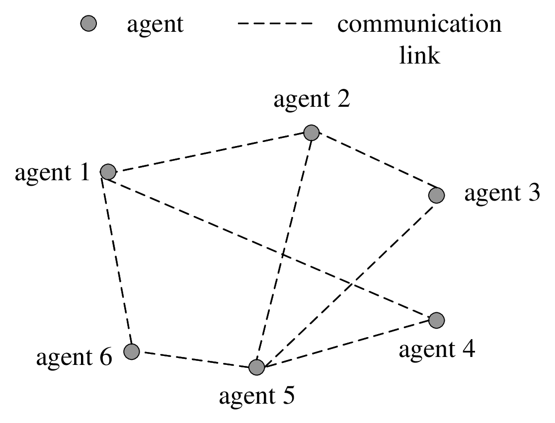
To solve the optimization problem (20), fiα​k​(𝒙~)f_{i}^{\alpha k}(\tilde{\bm{x}}) was set to fiα​k​(𝒙~)=12​𝒙~T​𝒙~+(𝒃ik)T​𝒙~f_{i}^{\alpha k}(\tilde{\bm{x}})=\frac{1}{2}\tilde{\bm{x}}^{T}\tilde{\bm{x}}+(\bm{b}_{i}^{k})^{T}\tilde{\bm{x}} for our approach in the simulations, where 𝒃ik\bm{b}_{i}^{k} was set to 𝒃ik=1k+1​𝒄i+𝒅i\bm{b}_{i}^{k}=\frac{1}{k+1}\bm{c}_{i}+\bm{d}_{i} with 𝒄i∈ℝn\bm{c}_{i}\in\mathbb{R}^{n} and 𝒅i∈ℝn\bm{d}_{i}\in\mathbb{R}^{n} being constants private to agent ii. Fig. 4 visualizes the evolution of 𝒙iα\bm{x}_{i}^{\alpha} and 𝒙iβ\bm{x}_{i}^{\beta} (i=1,2,…,6)(i=1,2,...,6) in one specific run where the network deployment is illustrated in Fig. 3. All 𝒙iα\bm{x}_{i}^{\alpha} and 𝒙iβ\bm{x}_{i}^{\beta} (i=1,2,…,6)(i=1,2,...,6) converged to the optimal solution 13.75813.758.

Refer to caption
Fig. 3: A network of six agents (N=6N=6).
Refer to caption
Fig. 4: The evolution of 𝒙iα\bm{x}_{i}^{\alpha} and 𝒙iβ\bm{x}_{i}^{\beta} in our approach.

VI-B Comparison with the algorithm in [18]

Under the network deployment in Fig. 3, we compared our privacy-preserving approach with the differential-privacy based algorithm in [18]. We simulated the algorithm in [18] under seven different privacy levels:

ϵ=0.2,1,10,20,30,50,100.\epsilon=0.2,1,10,20,30,50,100.

In the objective function (20), 𝒚i\bm{y}_{i} was set to 𝒚i=[0.1×(i−1)+0.1;0.1×(i−1)+0.2]\bm{y}_{i}=[0.1\times(i-1)+0.1;0.1\times(i-1)+0.2]. The domain of optimization for the algorithm in [18] was set to 𝒳={(x,y)∈ℝ2|x2+y2≤1}\mathcal{X}=\{(x,y)\in\mathbb{R}^{2}|x^{2}+y^{2}\leq 1\}. Note that the optimal solution [0.35;0.45][0.35;0.45] resided in 𝒳\mathcal{X}. Detailed parameter settings for the algorithm in [18] were given as n=2n=2, c=0.5c=0.5, q=0.8q=0.8, p=0.9p=0.9, and

ai​j={0.2j∈𝒩i,0j∉𝒩i,j≠i,1−∑j∈𝒩iai​ji=j,\displaystyle a_{ij}=\left\{\begin{aligned} 0.2\qquad\qquad\qquad&j\in\mathcal{N}_{i},\\ 0\qquad\qquad\qquad&j\notin\mathcal{N}_{i},j\neq i,\\ 1-\sum\limits_{j\in\mathcal{N}_{i}}a_{ij}\qquad&i=j,\end{aligned}\right. (22)

for i=1,2,…,6i=1,2,...,6. In addition, the performance index dd in [18] was used to quantify the optimization error here, which was computed as the average value of squared distances with respect to the optimal solution over MM runs [18], i.e.,

d=∑i=16∑l=1M∥𝒙il−[0.35;0.45]∥26​M.d=\frac{\sum\limits_{i=1}^{6}\sum\limits_{l=1}^{M}\parallel\bm{x}_{i}^{l}-[0.35;0.45]\parallel^{2}}{6M}.

Here 𝒙il\bm{x}_{i}^{l} is the obtained solution of agent ii in the llth run. For our approach, 𝒙il\bm{x}_{i}^{l} was calculated as the average of 𝒙iα​l\bm{x}_{i}^{\alpha l} and 𝒙iβ​l\bm{x}_{i}^{\beta l}.

Simulation results from 5,000 runs showed that our approach converged to [0.35;0.45][0.35;0.45] with an error d=5.1×10⁻⁴d=5.1\times 10^{-4}, which is negligible compared with the simulation results under the algorithm in [18] (cf. Fig. 5, where each differential privacy level was implemented for 5,000 times). The results confirm the trade-off between privacy and accuracy in differential-privacy based approaches.

Refer to caption
Fig. 5: The comparison of our approach with the algorithm in [18] in terms of optimization error.

VII Conclusions

In this paper, we proposed a novel approach to enabling privacy-preservation in decentralized optimization based on function decomposition, which neither compromises the optimality of optimization nor relies on an aggregator or third party. Theoretical analysis confirms that an honest-but-curious adversary cannot infer the information of neighboring agents even by recording and analyzing the information exchanged in multiple iterations. In addition, our approach can also avoid an external eavesdropper from inferring the information of participating agents. Numerical simulation results confirmed the effectiveness of the proposed approach.

APPENDIX

VII-A Proof of Theorem 2

From Lemma 3, we can obtain

1+δk∥𝒚k−𝒚k∗∥H≤∥𝒚0−𝒚0∗∥H+∑s=0k−11+δsp(s).\displaystyle\sqrt{1+\delta}^{k}\parallel\bm{y}^{k}-\bm{y}^{k*}\parallel_{H}\leq\parallel\bm{y}^{0}-\bm{y}^{0*}\parallel_{H}+\sum_{s=0}^{k-1}\sqrt{1+\delta}^{s}p(s). (23)

Dividing both sides by 1+δk\sqrt{1+\delta}^{k}, we have

∥𝒚k−𝒚k∗∥H≤∥𝒚0−𝒚0∗∥H1+δk+∑s=0k−111+δk−sp(s).\displaystyle\parallel\bm{y}^{k}-\bm{y}^{k*}\parallel_{H}\leq\frac{\parallel\bm{y}^{0}-\bm{y}^{0*}\parallel_{H}}{\sqrt{1+\delta}^{k}}+\sum_{s=0}^{k-1}\frac{1}{\sqrt{1+\delta}^{k-s}}p(s). (24)

It is clear limk→∞∥𝒚0−𝒚0∗∥H1+δk=0\lim\limits_{k\to\infty}\frac{\parallel\bm{y}^{0}-\bm{y}^{0*}\parallel_{H}}{\sqrt{1+\delta}^{k}}=0 due to δ>0\delta>0. Now our main goal is to prove limk→∞∑s=0k−111+δk−s​p​(s)=0\lim\limits_{k\to\infty}\sum_{s=0}^{k-1}\frac{1}{\sqrt{1+\delta}^{k-s}}p(s)=0. Recall that in Assumption 3 we have limk→∞fiα​k→fiα∗\lim\limits_{k\to\infty}f_{i}^{\alpha k}\to f_{i}^{\alpha*}. Therefore, we have limk→∞hik→hi∗\lim\limits_{k\to\infty}h_{i}^{k}\to h_{i}^{*} for all i=1,2,…,2​Ni=1,2,\dots,2N, i.e., hikh_{i}^{k} converges to a fixed function hi∗h_{i}^{*} (hkh^{k} converges to a fixed function h∗h^{*}). On the other hand, we have

p(k)=1ρ​Amin∥▽hk+1(𝒙∗)−▽hk(𝒙∗)∥.\displaystyle p(k)=\frac{1}{\sqrt{\rho A_{\min}}}\parallel\triangledown h^{k+1}(\bm{x}^{*})-\triangledown h^{k}(\bm{x}^{*})\parallel. (25)

As a result of the convergence of hkh^{k}, we have limk→∞p⁡(k)=0\lim\limits_{k\to\infty}p(k)=0. Therefore, we have that p⁡(k)p(k) is bounded, i,e., there exists a BB such that p⁡(k)≤B,∀kp(k)\leq B,\forall k. In addition, we have

∀ε1>0,∃N1∈ℕ+, s.t. ​|p⁡(k)|≤ε1,∀k≥N1,\forall\varepsilon_{1}>0,\quad\exists N_{1}\in\mathbb{N}^{+},\text{\quad s.t.\quad}|p(k)|\leq\varepsilon_{1},\quad\forall k\geq N_{1},

where ℕ+\mathbb{N}^{+} is the set of positive integers. Further letting η=11+δ\eta=\frac{1}{\sqrt{1+\delta}} and F⁡(k)=∑s=0k−111+δk−s​p​(s)F(k)=\sum_{s=0}^{k-1}\frac{1}{\sqrt{1+\delta}^{k-s}}p(s), we have η∈(0,1)\eta\in(0,1) and

F⁡(k)\displaystyle F(k) =∑s=0k−1ηk−s​p​(s)\displaystyle=\sum_{s=0}^{k-1}\eta^{k-s}p(s) (26)
=∑s=0N1ηk−s​p​(s)+∑s=N1+1k−1ηk−s​p​(s)\displaystyle=\sum_{s=0}^{N_{1}}\eta^{k-s}p(s)+\sum_{s=N_{1}+1}^{k-1}\eta^{k-s}p(s)
≤B​∑s=0N1ηk−s+ε1​∑s=N1+1k−1ηk−s\displaystyle\leq B\sum_{s=0}^{N_{1}}\eta^{k-s}+\varepsilon_{1}\sum_{s=N_{1}+1}^{k-1}\eta^{k-s}
=B​ηk​η−N1−η1−η+ε1​η−ηk−N1−11−η\displaystyle=B\eta^{k}\frac{\eta^{-N_{1}}-\eta}{1-\eta}+\varepsilon_{1}\frac{\eta-\eta^{k-N_{1}-1}}{1-\eta}
≤B​ηk​η−N1−η1−η+ε1​η1−η\displaystyle\leq B\eta^{k}\frac{\eta^{-N_{1}}-\eta}{1-\eta}+\varepsilon_{1}\frac{\eta}{1-\eta}

for k≥N1+2k\geq N_{1}+2.

Recalling η∈(0,1)\eta\in(0,1), we have limk→∞B​ηk​η−N1−η1−η=0\lim\limits_{k\to\infty}B\eta^{k}\frac{\eta^{-N_{1}}-\eta}{1-\eta}=0 and

∀ε=ε1>0,∃N2∈ℕ+,\displaystyle\forall\varepsilon=\varepsilon_{1}>0,\quad\exists N_{2}\in\mathbb{N}^{+}, (27)
s.t. |Bηkη−N1−η1−η|≤ε1,∀k≥N2,\displaystyle\text{s.t.\quad}|B\eta^{k}\frac{\eta^{-N_{1}}-\eta}{1-\eta}|\leq\varepsilon_{1},\quad\forall k\geq N_{2},

Therefore, we can obtain

∀ε=ε1>0,∃N=max{N1,N2},\displaystyle\forall\varepsilon=\varepsilon_{1}>0,\quad\exists N=\max\{N_{1},N_{2}\}, (28)
s.t. |F(k)|≤ε1+ε1η1−η=11−ηε1,∀k≥N,\displaystyle\text{s.t.\quad}|F(k)|\leq\varepsilon_{1}+\varepsilon_{1}\frac{\eta}{1-\eta}=\frac{1}{1-\eta}\varepsilon_{1},\quad\forall k\geq N,

which proves that limk→∞F⁡(k)=0\lim\limits_{k\to\infty}F(k)=0. Then according to (24), we have limk→∞∥𝒚k−𝒚k∗∥H=0\lim\limits_{k\to\infty}\parallel\bm{y}^{k}-\bm{y}^{k*}\parallel_{H}=0. Since ∥𝒙k−𝒙∗∥Q≤∥𝒚k−𝒚k∗∥H\parallel\bm{x}^{k}-\bm{x}^{*}\parallel_{Q}\leq\parallel\bm{y}^{k}-\bm{y}^{k*}\parallel_{H}, we have limk→∞∥𝒙k−𝒙∗∥Q=0\lim\limits_{k\to\infty}\parallel\bm{x}^{k}-\bm{x}^{*}\parallel_{Q}=0 as well, which completes the proof.

References

  • [1] J. Lin, A. S. Morse, and B. Anderson. The multi-agent rendezvous problem-the asynchronous case. In 43rd IEEE Conference on Decision and Control, volume 2, pages 1926–1931, 2004.
  • [2] C. Cortes and V. Vapnik. Support-vector networks. Machine learning, 20(3):273–297, 1995.
  • [3] T. Zhang and Q. Zhu. Dynamic differential privacy for ADMM-based distributed classification learning. IEEE Transactions on Information Forensics and Security, 12(1):172–187, 2017.
  • [4] C. L. Zhang and Y. Wang. Distributed event localization via alternating direction method of multipliers. IEEE Transactions on Mobile Computing, 17(2):348–361, 2018.
  • [5] G. Mateos, J. A. Bazerque, and G. B. Giannakis. Distributed sparse linear regression. IEEE Transactions on Signal Processing, 58(10):5262–5276, 2010.
  • [6] J. Liu, J. Chen, and J. Ye. Large-scale sparse logistic regression. In Proceedings of the 15th ACM SIGKDD international conference on Knowledge discovery and data mining, pages 547–556, 2009.
  • [7] A. Nedic and A. Ozdaglar. Distributed subgradient methods for multi-agent optimization. IEEE Transactions on Automatic Control, 54(1):48–61, 2009.
  • [8] B. S. He, H. K. Xu, and X. M. Yuan. On the proximal jacobian decomposition of ALM for multiple-block separable convex minimization problems and its relationship to ADMM. Journal of Scientific Computing, 66(3):1204–1217, 2016.
  • [9] S. Boyd, N. Parikh, E. Chu, B. Peleato, and J. Eckstein. Distributed optimization and statistical learning via the alternating direction method of multipliers. Foundations and Trends in Machine Learning, 3(1):1–122, 2011.
  • [10] Q. Ling and A. Ribeiro. Decentralized dynamic optimization through the alternating direction method of multipliers. In 2013 IEEE 14th Workshop on Signal Processing Advances in Wireless Communications, pages 170–174, 2013.
  • [11] Q. Ling, Y. Liu, W. Shi, and Z. Tian. Weighted ADMM for fast decentralized network optimization. IEEE Transactions on Signal Processing, 64(22):5930–5942, 2016.
  • [12] W. Shi, Q. Ling, K. Yuan, G. Wu, and W. Yin. On the linear convergence of the ADMM in decentralized consensus optimization. IEEE Transactions on Signal Processing, 62(7):1750–1761, 2014.
  • [13] M. Maros and J. Jaldén. On the Q-linear convergence of distributed generalized ADMM under non-strongly convex function components. arXiv preprint arXiv:1805.01660, 2018.
  • [14] A. Al-Anwar, Y. Shoukry, S. Chakraborty, P. Martin, P. Tabuada, and M. B. Srivastava. PrOLoc: resilient localization with private observers using partial homomorphic encryption. In IPSN, pages 41–52, 2017.
  • [15] Y. Mo and R. M. Murray. Privacy preserving average consensus. IEEE Transactions on Automatic Control, 62(2):753–765, 2017.
  • [16] P. C. Weeraddana, G. Athanasiou, M. Jakobsson, C. Fischione, and J. Baras. Per-se privacy preserving distributed optimization. arXiv preprint arXiv:1210.3283, 2012.
  • [17] M. H. DeGroot. Reaching a consensus. Journal of the American Statistical Association, 69(345):118–121, 1974.
  • [18] Z. Huang, S. Mitra, and N. Vaidya. Differentially private distributed optimization. In Proceedings of the 2015 International Conference on Distributed Computing and Networking, page 4, 2015.
  • [19] S. Han, U. Topcu, and G. J. Pappas. Differentially private distributed constrained optimization. IEEE Transactions on Automatic Control, 62(1):50–64, 2017.
  • [20] E. Nozari, P. Tallapragada, and J. Cortes. Differentially private distributed convex optimization via functional perturbation. IEEE Transactions on Control of Network Systems, 2016.
  • [21] X. R. Zhang, M. M. Khalili, and M. Liu. Improving the privacy and accuracy of ADMM-based distributed algorithms. arXiv preprint arXiv:1806.02246, 2018.
  • [22] M. T. Hale and M. Egerstedt. Differentially private cloud-based multi-agent optimization with constraints. In American Control Conference, pages 1235–1240, 2015.
  • [23] M. T. Hale and M. Egerstedt. Cloud-enabled differentially private multi-agent optimization with constraints. IEEE Transactions on Control of Network Systems, 2017.
  • [24] Z. Xu and Q. Zhu. Secure and resilient control design for cloud enabled networked control systems. In Proceedings of the First ACM Workshop on Cyber-Physical Systems-Security and/or PrivaCy, pages 31–42, 2015.
  • [25] A. C. Yao. Protocols for secure computations. In 23rd Annual Symposium on Foundations of Computer Science, pages 160–164, 1982.
  • [26] C. L. Zhang, M. Ahmad, and Y. Wang. ADMM based privacy-preserving decentralized optimization. IEEE Transactions on Information Forensics and Security, 2018.
  • [27] R. L. Lagendijk, Z. Erkin, and M. Barni. Encrypted signal processing for privacy protection: Conveying the utility of homomorphic encryption and multiparty computation. IEEE Signal Processing Magazine, 30(1):82–105, 2013.
  • [28] S. Pequito, S. Kar, S. Sundaram, and A. P. Aguiar. Design of communication networks for distributed computation with privacy guarantees. In 2014 IEEE 53rd Annual Conference on Decision and Control, pages 1370–1376, 2014.
  • [29] A. Alaeddini, K. Morgansen, and M. Mesbahi. Adaptive communication networks with privacy guarantees. In American Control Conference, pages 4460–4465. IEEE, 2017.
  • [30] F. Yan, S. Sundaram, S. Vishwanathan, and Y. Qi. Distributed autonomous online learning: Regrets and intrinsic privacy-preserving properties. IEEE Transactions on Knowledge and Data Engineering, 25(11):2483–2493, 2013.
  • [31] Y. Lou, L. Yu, S. Wang, and P. Yi. Privacy preservation in distributed subgradient optimization algorithms. IEEE Transactions on Cybernetics, 2017.
  • [32] F. Li, B. Luo, and P. Liu. Secure information aggregation for smart grids using homomorphic encryption. In 2010 First IEEE International Conference on Smart Grid Communications, pages 327–332, 2010.
  • [33] W. Deng, M. Lai, Z. Peng, and W. Yin. Parallel multi-block ADMM with o(1/k) convergence. Journal of Scientific Computing, 71(2):712–736, 2017.
  • [34] E. Wei and A. Ozdaglar. Distributed alternating direction method of multipliers. In Proceedings of the 51st IEEE Conference on Decision and Control, pages 5445–5450, 2012.
  • [35] Q. Ling and A. Ribeiro. Decentralized dynamic optimization through the alternating direction method of multipliers. IEEE Transactions on Signal Processing, 62(5):1185–1197, 2014.
  • [36] C. L. Zhang, H. Gao, and Y. Wang. Privacy-preserving decentralized optimization via decomposition. arXiv preprint arXiv:1808.09566, 2018.

Supplemental Materials: Privacy-preserving Decentralized Optimization via Decomposition

VII-B Proof of Lemma 1

According to the update rules in (7) and (8) , we have

▽​hik+1​(𝒙ik+1)+∑j∈𝒩i(𝝀i,jk+ρ⁡(𝒙ik+1−𝒙jk))+γi​ρ​(𝒙ik+1−𝒙ik)=𝟎\displaystyle\triangledown h_{i}^{k+1}(\bm{x}_{i}^{k+1})+\sum_{j\in\mathcal{N}_{i}}(\bm{\lambda}_{i,j}^{k}+\rho(\bm{x}_{i}^{k+1}-\bm{x}_{j}^{k}))+\gamma_{i}\rho(\bm{x}_{i}^{k+1}-\bm{x}_{i}^{k})=\bm{0} (29)

for all i=1,2,…,2​Ni=1,2,\ldots,2N.

Let (𝒙∗,𝝀k∗)(\bm{x}^{*},\bm{\lambda}^{k*}) be the Karush-Kuhn-Tucker (KKT) points for (14) at iteration kk, we have

−AiT𝝀k∗\displaystyle-A_{i}^{T}\bm{\lambda}^{k*} =▽​hik​(𝒙i∗)\displaystyle=\triangledown h_{i}^{k}(\bm{x}_{i}^{*}) (30)
A​𝒙∗\displaystyle A\bm{x}^{*} =𝟎\displaystyle=\bm{0}

where AiA_{i} indicates the columns of AA corresponding to agent ii. It is worth noting that since ∑i=12​Nhik​(𝒙i)\sum\limits_{i=1}^{2N}h_{i}^{k}(\bm{x}_{i}) is strongly convex, 𝒙∗\bm{x}^{*} is the optimal solution to (14).

Since each hikh_{i}^{k} is strongly convex, we have

(▽hik+1(𝒙ik+1)−▽hik+1(𝒙i∗))T(𝒙ik+1−𝒙i∗)≥mf∥𝒙ik+1−𝒙i∗∥2.\displaystyle(\triangledown h_{i}^{k+1}(\bm{x}_{i}^{k+1})-\triangledown h_{i}^{k+1}(\bm{x}_{i}^{*}))^{T}(\bm{x}_{i}^{k+1}-\bm{x}_{i}^{*})\geq m_{f}\parallel\bm{x}_{i}^{k+1}-\bm{x}_{i}^{*}\parallel^{2}. (31)

Combining the above equation with (29) and (30), we have

(−∑j∈𝒩i(𝝀i,jk+ρ(𝒙ik+1−𝒙jk))−γiρ(𝒙ik+1−𝒙ik)+AiT𝝀k+1∗)T(𝒙ik+1−𝒙i∗)≥mf∥𝒙ik+1−𝒙i∗∥2.\displaystyle(-\sum_{j\in\mathcal{N}_{i}}(\bm{\lambda}_{i,j}^{k}+\rho(\bm{x}_{i}^{k+1}-\bm{x}_{j}^{k}))-\gamma_{i}\rho(\bm{x}_{i}^{k+1}-\bm{x}_{i}^{k})+A_{i}^{T}\bm{\lambda}^{k+1*})^{T}(\bm{x}_{i}^{k+1}-\bm{x}_{i}^{*})\geq m_{f}\parallel\bm{x}_{i}^{k+1}-\bm{x}_{i}^{*}\parallel^{2}. (32)

Noting that 𝝀i,jk+1=𝝀i,jk+ρ⁡(𝒙ik+1−𝒙jk+1)\bm{\lambda}_{i,j}^{k+1}=\bm{\lambda}_{i,j}^{k}+\rho(\bm{x}_{i}^{k+1}-\bm{x}_{j}^{k+1}), one has

(−∑j∈𝒩i(𝝀i,jk+1+ρ(𝒙jk+1−𝒙jk))−γiρ(𝒙ik+1−𝒙ik)+AiT𝝀k+1∗)T(𝒙ik+1−𝒙i∗)≥mf∥𝒙ik+1−𝒙i∗∥2.\displaystyle(-\sum_{j\in\mathcal{N}_{i}}(\bm{\lambda}_{i,j}^{k+1}+\rho(\bm{x}_{j}^{k+1}-\bm{x}_{j}^{k}))-\gamma_{i}\rho(\bm{x}_{i}^{k+1}-\bm{x}_{i}^{k})+A_{i}^{T}\bm{\lambda}^{k+1*})^{T}(\bm{x}_{i}^{k+1}-\bm{x}_{i}^{*})\geq m_{f}\parallel\bm{x}_{i}^{k+1}-\bm{x}_{i}^{*}\parallel^{2}. (33)

Based on the definition of AA, DD, and UU, one can further have

∑j∈𝒩i𝝀i,jk+1=AiT​𝝀k+1,\displaystyle\sum\limits_{j\in\mathcal{N}_{i}}\bm{\lambda}_{i,j}^{k+1}=A_{i}^{T}\bm{\lambda}^{k+1}, (34)
∑j∈𝒩i(𝒙jk+1−𝒙jk)=(D−AT​A)iT​(𝒙k+1−𝒙k),\displaystyle\sum\limits_{j\in\mathcal{N}_{i}}(\bm{x}_{j}^{k+1}-\bm{x}_{j}^{k})=(D-A^{T}A)_{i}^{T}(\bm{x}^{k+1}-\bm{x}^{k}), (35)
γi​ρ​(𝒙ik+1−𝒙ik)=ρ​Ui​(𝒙k+1−𝒙k).\displaystyle\gamma_{i}\rho(\bm{x}_{i}^{k+1}-\bm{x}_{i}^{k})=\rho U_{i}(\bm{x}^{k+1}-\bm{x}^{k}). (36)

Recall that Q=D−AT​A+UQ=D-A^{T}A+U and Q=QTQ=Q^{T}, we can combine (33) with the above three equations to obtain

(−AiT(𝝀k+1−𝝀k+1∗)−ρQiT(𝒙k+1−𝒙k))T⋅(𝒙ik+1−𝒙i∗)≥mf∥𝒙ik+1−𝒙i∗∥2.\displaystyle(-A_{i}^{T}(\bm{\lambda}^{k+1}-\bm{\lambda}^{k+1*})-\rho Q_{i}^{T}(\bm{x}^{k+1}-\bm{x}^{k}))^{T}\bm{\cdot}(\bm{x}_{i}^{k+1}-\bm{x}_{i}^{*})\geq m_{f}\parallel\bm{x}_{i}^{k+1}-\bm{x}_{i}^{*}\parallel^{2}. (37)

Summing both sides of (37) over i=1,2,…,2​Ni=1,2,\ldots,2N and using

∑i=12​N(𝒙ik+1−𝒙i∗)T(Ai)T(𝝀k+1−𝝀k+1∗)=(𝒙k+1−𝒙∗)TAT(𝝀k+1−𝝀k+1∗)\displaystyle\sum\limits_{i=1}^{2N}(\bm{x}_{i}^{k+1}-\bm{x}_{i}^{*})^{T}(A_{i})^{T}(\bm{\lambda}^{k+1}-\bm{\lambda}^{k+1*})=(\bm{x}^{k+1}-\bm{x}^{*})^{T}A^{T}(\bm{\lambda}^{k+1}-\bm{\lambda}^{k+1*})
∑i=12​N(𝒙ik+1−𝒙i∗)T​ρ​QiT​(𝒙k+1−𝒙k)=ρ​(𝒙k+1−𝒙∗)T​QT​(𝒙k+1−𝒙k)\displaystyle\sum\limits_{i=1}^{2N}(\bm{x}_{i}^{k+1}-\bm{x}_{i}^{*})^{T}\rho Q_{i}^{T}(\bm{x}^{k+1}-\bm{x}^{k})=\rho(\bm{x}^{k+1}-\bm{x}^{*})^{T}Q^{T}(\bm{x}^{k+1}-\bm{x}^{k})

we have

−(𝒙k+1−𝒙∗)TAT(𝝀k+1−𝝀k+1∗)−ρ(𝒙k+1−𝒙∗)TQT(𝒙k+1−𝒙k)≥mf∥𝒙k+1−𝒙∗∥2\displaystyle-(\bm{x}^{k+1}-\bm{x}^{*})^{T}A^{T}(\bm{\lambda}^{k+1}-\bm{\lambda}^{k+1*})-\rho(\bm{x}^{k+1}-\bm{x}^{*})^{T}Q^{T}(\bm{x}^{k+1}-\bm{x}^{k})\geq m_{f}\parallel\bm{x}^{k+1}-\bm{x}^{*}\parallel^{2} (38)

Moreover, the following equalities can be obtained by using algebraic manipulations:

(𝒙k+1−𝒙∗)TQT(𝒙k+1−𝒙k)=12∥𝒙k+1−𝒙k∥Q2+12(∥𝒙k+1−𝒙∗∥Q2−∥𝒙k−𝒙∗∥Q2),\displaystyle(\bm{x}^{k+1}-\bm{x}^{*})^{T}Q^{T}(\bm{x}^{k+1}-\bm{x}^{k})=\frac{1}{2}\parallel\bm{x}^{k+1}-\bm{x}^{k}\parallel_{Q}^{2}+\frac{1}{2}(\parallel\bm{x}^{k+1}-\bm{x}^{*}\parallel_{Q}^{2}-\parallel\bm{x}^{k}-\bm{x}^{*}\parallel_{Q}^{2}), (39)
(𝒙k+1−𝒙∗)TAT(𝝀k+1−𝝀k+1∗)=1ρ(𝝀k+1−𝝀k)T(𝝀k+1−𝝀k+1∗)\displaystyle(\bm{x}^{k+1}-\bm{x}^{*})^{T}A^{T}(\bm{\lambda}^{k+1}-\bm{\lambda}^{k+1*})=\frac{1}{\rho}(\bm{\lambda}^{k+1}-\bm{\lambda}^{k})^{T}(\bm{\lambda}^{k+1}-\bm{\lambda}^{k+1*}) (40)
1ρ(𝝀k+1−𝝀k)T(𝝀k+1−𝝀k+1∗)=12​ρ∥𝝀k+1−𝝀k∥2−12​ρ∥𝝀k−𝝀k+1∗∥2+12​ρ∥𝝀k+1−𝝀k+1∗∥2\displaystyle\frac{1}{\rho}(\bm{\lambda}^{k+1}-\bm{\lambda}^{k})^{T}(\bm{\lambda}^{k+1}-\bm{\lambda}^{k+1*})=\frac{1}{2\rho}\parallel\bm{\lambda}^{k+1}-\bm{\lambda}^{k}\parallel^{2}-\frac{1}{2\rho}\parallel\bm{\lambda}^{k}-\bm{\lambda}^{k+1*}\parallel^{2}+\frac{1}{2\rho}\parallel\bm{\lambda}^{k+1}-\bm{\lambda}^{k+1*}\parallel^{2} (41)

Based on the above three inequities, (38) can be rewritten as

mf∥𝒙k+1−𝒙∗∥2≤\displaystyle m_{f}\parallel\bm{x}^{k+1}-\bm{x}^{*}\parallel^{2}\leq −ρ2∥𝒙k+1−𝒙∗∥Q2−12​ρ∥𝝀k+1−𝝀k+1∗∥2+ρ2∥𝒙k−𝒙∗∥Q2+12​ρ∥𝝀k−𝝀k+1∗∥2\displaystyle-\frac{\rho}{2}\parallel\bm{x}^{k+1}-\bm{x}^{*}\parallel_{Q}^{2}-\frac{1}{2\rho}\parallel\bm{\lambda}^{k+1}-\bm{\lambda}^{k+1*}\parallel^{2}+\frac{\rho}{2}\parallel\bm{x}^{k}-\bm{x}^{*}\parallel_{Q}^{2}+\frac{1}{2\rho}\parallel\bm{\lambda}^{k}-\bm{\lambda}^{k+1*}\parallel^{2} (42)
−ρ2∥𝒙k+1−𝒙k∥Q2−12​ρ∥𝝀k+1−𝝀k∥2\displaystyle-\frac{\rho}{2}\parallel\bm{x}^{k+1}-\bm{x}^{k}\parallel_{Q}^{2}-\frac{1}{2\rho}\parallel\bm{\lambda}^{k+1}-\bm{\lambda}^{k}\parallel^{2}

Recall that H=diag⁡{ρ​Q,1ρ​I|E|​n}H={\rm diag}\{\rho Q,\frac{1}{\rho}I_{|E|n}\} and 𝒚k=[𝒙k​T,𝝀k​T]T\bm{y}^{k}=[\bm{x}^{kT},\bm{\lambda}^{kT}]^{T}. The above inequality can be simplified as

2mf∥𝒙k+1−𝒙∗∥2≤∥𝒚k−𝒚k+1∗∥H2−∥𝒚k+1−𝒚k+1∗∥H2−∥𝒚k+1−𝒚k∥H2\displaystyle 2m_{f}\parallel\bm{x}^{k+1}-\bm{x}^{*}\parallel^{2}\leq\parallel\bm{y}^{k}-\bm{y}^{k+1*}\parallel_{H}^{2}-\parallel\bm{y}^{k+1}-\bm{y}^{k+1*}\parallel_{H}^{2}-\parallel\bm{y}^{k+1}-\bm{y}^{k}\parallel_{H}^{2} (43)

On the other hand, note that for any constant u>1u>1, the following relationship is true [35]

(u−1)∥𝒂−𝒃∥2≥(1−1u)∥𝒃∥2−∥𝒂∥2\displaystyle(u-1)\parallel\bm{a}-\bm{b}\parallel^{2}\geq(1-\frac{1}{u})\parallel\bm{b}\parallel^{2}-\parallel\bm{a}\parallel^{2} (44)

So we have

(u−1)∥▽hk+1(𝒙k+1)−▽hk+1(𝒙∗)∥2\displaystyle(u-1)\parallel\triangledown h^{k+1}(\bm{x}^{k+1})-\triangledown h^{k+1}(\bm{x}^{*})\parallel^{2} =(u−1)∥AT(𝝀k+1−𝝀k+1∗)+ρQT(𝒙k+1−𝒙k)∥2\displaystyle=(u-1)\parallel A^{T}(\bm{\lambda}^{k+1}-\bm{\lambda}^{k+1*})+\rho Q^{T}(\bm{x}^{k+1}-\bm{x}^{k})\parallel^{2} (45)
≥u−1u∥AT(𝝀k+1−𝝀k+1∗)∥2−∥ρQT(𝒙k+1−𝒙k)∥2\displaystyle\geq\frac{u-1}{u}\parallel A^{T}(\bm{\lambda}^{k+1}-\bm{\lambda}^{k+1*})\parallel^{2}-\parallel\rho Q^{T}(\bm{x}^{k+1}-\bm{x}^{k})\parallel^{2}

Since 𝝀k+1\bm{\lambda}^{k+1} and 𝝀k+1∗\bm{\lambda}^{k+1*} lie in the column space of of AA, we have [35]

∥AT(𝝀k+1−𝝀k+1∗)∥2≥Amin∥𝝀k+1−𝝀k+1∗∥2\displaystyle\parallel A^{T}(\bm{\lambda}^{k+1}-\bm{\lambda}^{k+1*})\parallel^{2}\geq A_{\min}\parallel\bm{\lambda}^{k+1}-\bm{\lambda}^{k+1*}\parallel^{2} (46)
∥ρQT(𝒙k+1−𝒙k)∥2≤ρ2Qmax∥𝒙k+1−𝒙k∥Q2\displaystyle\parallel\rho Q^{T}(\bm{x}^{k+1}-\bm{x}^{k})\parallel^{2}\leq\rho^{2}Q_{\max}\parallel\bm{x}^{k+1}-\bm{x}^{k}\parallel_{Q}^{2}

where QmaxQ_{\max} is the largest eigenvalue of QQ, AminA_{\min} is the smallest nonzero eigenvalue of AT​AA^{T}A.

In addition, given that ∥▽hk+1(𝒙k+1)−▽hk+1(𝒙∗)∥2≤L2∥𝒙k+1−𝒙∗∥2\parallel\triangledown h^{k+1}(\bm{x}^{k+1})-\triangledown h^{k+1}(\bm{x}^{*})\parallel^{2}\leq L^{2}\parallel\bm{x}^{k+1}-\bm{x}^{*}\parallel^{2} is true according to Assumption 3, using (46) and (45), we can obtain

(u−1)L2∥𝒙k+1−𝒙∗∥2≥(u−1)​Aminu∥𝝀k+1−𝝀k+1∗∥2−ρ2Qmax∥𝒙k+1−𝒙k∥Q2\displaystyle(u-1)L^{2}\parallel\bm{x}^{k+1}-\bm{x}^{*}\parallel^{2}\geq\frac{(u-1)A_{\min}}{u}\parallel\bm{\lambda}^{k+1}-\bm{\lambda}^{k+1*}\parallel^{2}-\rho^{2}Q_{\max}\parallel\bm{x}^{k+1}-\bm{x}^{k}\parallel_{Q}^{2} (47)

Using algebraic manipulations, the above inequality can be rewritten as

u​Qmax(u−1)​Aminρ∥𝒙k+1−𝒙k∥Q2+u​L2ρ​Amin∥𝒙k+1−𝒙∗∥2≥1ρ∥𝝀k+1−𝝀k+1∗∥2\displaystyle\frac{uQ_{\max}}{(u-1)A_{\min}}\rho\parallel\bm{x}^{k+1}-\bm{x}^{k}\parallel_{Q}^{2}+\frac{uL^{2}}{\rho A_{\min}}\parallel\bm{x}^{k+1}-\bm{x}^{*}\parallel^{2}\geq\frac{1}{\rho}\parallel\bm{\lambda}^{k+1}-\bm{\lambda}^{k+1*}\parallel^{2} (48)

Adding u​Qmax(u−1)​Amin1ρ∥𝝀k+1−𝝀k∥2\frac{uQ_{\max}}{(u-1)A_{\min}}\frac{1}{\rho}\parallel\bm{\lambda}^{k+1}-\bm{\lambda}^{k}\parallel^{2} and ρQmax∥𝒙k+1−𝒙∗∥2\rho Q_{\max}\parallel\bm{x}^{k+1}-\bm{x}^{*}\parallel^{2} to the left hand side of the above inequality, and adding ρ∥𝒙k+1−𝒙∗∥Q2\rho\parallel\bm{x}^{k+1}-\bm{x}^{*}\parallel_{Q}^{2} to the right hand side, we obtain the following inequality based on the fact ρ∥𝒙k+1−𝒙∗∥Q2≤ρQmax∥𝒙k+1−𝒙∗∥2\rho\parallel\bm{x}^{k+1}-\bm{x}^{*}\parallel_{Q}^{2}\leq\rho Q_{\max}\parallel\bm{x}^{k+1}-\bm{x}^{*}\parallel^{2}:

u​Qmax(u−1)​Amin(ρ∥𝒙k+1−𝒙k∥Q2+1ρ∥𝝀k+1−𝝀k∥2)+(u​L2ρ​Amin+ρQmax)∥𝒙k+1−𝒙∗∥2\displaystyle\frac{uQ_{\max}}{(u-1)A_{\min}}(\rho\parallel\bm{x}^{k+1}-\bm{x}^{k}\parallel_{Q}^{2}+\frac{1}{\rho}\parallel\bm{\lambda}^{k+1}-\bm{\lambda}^{k}\parallel^{2})+(\frac{uL^{2}}{\rho A_{\min}}+\rho Q_{\max})\parallel\bm{x}^{k+1}-\bm{x}^{*}\parallel^{2} (49)
≥1ρ∥𝝀k+1−𝝀k+1∗∥2+ρ∥𝒙k+1−𝒙∗∥Q2\displaystyle\geq\frac{1}{\rho}\parallel\bm{\lambda}^{k+1}-\bm{\lambda}^{k+1*}\parallel^{2}+\rho\parallel\bm{x}^{k+1}-\bm{x}^{*}\parallel_{Q}^{2}

Let

δ=min⁡{(u−1)​Aminu​Qmax,2​mf​Amin​ρu​L2+ρ2​Amin​Qmax}\displaystyle\delta=\min\{\frac{(u-1)A_{\min}}{uQ_{\max}},\frac{2m_{f}A_{\min}\rho}{uL^{2}+\rho^{2}A_{\min}Q_{\max}}\} (50)

Inequality (49) becomes

1δ∥𝒚k+1−𝒚k∥H2+2​mfδ∥𝒙k+1−𝒙∗∥2≥∥𝒚k+1−𝒚k+1∗∥H2\displaystyle\frac{1}{\delta}\parallel\bm{y}^{k+1}-\bm{y}^{k}\parallel_{H}^{2}+\frac{2m_{f}}{\delta}\parallel\bm{x}^{k+1}-\bm{x}^{*}\parallel^{2}\geq\parallel\bm{y}^{k+1}-\bm{y}^{k+1*}\parallel_{H}^{2} (51)

Based on (43) and (51), we can get

1δ∥𝒚k−𝒚k+1∗∥H2−1δ∥𝒚k+1−𝒚k+1∗∥H2≥∥𝒚k+1−𝒚k+1∗∥H2\displaystyle\frac{1}{\delta}\parallel\bm{y}^{k}-\bm{y}^{k+1*}\parallel_{H}^{2}-\frac{1}{\delta}\parallel\bm{y}^{k+1}-\bm{y}^{k+1*}\parallel_{H}^{2}\geq\parallel\bm{y}^{k+1}-\bm{y}^{k+1*}\parallel_{H}^{2} (52)

which proves Lemma 1.

VII-C Proof of Lemma 2

First, we have

∥𝒚k−𝒚k+1∗∥H−∥𝒚k−𝒚k∗∥H≤∥𝒚k+1∗−𝒚k∗∥H\displaystyle\parallel\bm{y}^{k}-\bm{y}^{k+1*}\parallel_{H}-\parallel\bm{y}^{k}-\bm{y}^{k*}\parallel_{H}\leq\parallel\bm{y}^{k+1*}-\bm{y}^{k*}\parallel_{H} (53)

On the other hand, we have

∥𝒚k+1∗−𝒚k∗∥H=1ρ∥𝝀k+1∗−𝝀k∗∥\displaystyle\parallel\bm{y}^{k+1*}-\bm{y}^{k*}\parallel_{H}=\frac{1}{\sqrt{\rho}}\parallel\bm{\lambda}^{k+1*}-\bm{\lambda}^{k*}\parallel (54)
∥AT(𝝀k+1∗−𝝀k∗)∥=∥▽hk+1(𝒙∗)−▽hk(𝒙∗)∥.\displaystyle\parallel A^{T}(\bm{\lambda}^{k+1*}-\bm{\lambda}^{k*})\parallel=\parallel\triangledown h^{k+1}(\bm{x}^{*})-\triangledown h^{k}(\bm{x}^{*})\parallel. (55)

Therefore, we can get the following inequality using (46)

∥𝝀k+1∗−𝝀k∗∥≤1Amin∥▽hk+1(𝒙∗)−▽hk(𝒙∗)∥.\displaystyle\parallel\bm{\lambda}^{k+1*}-\bm{\lambda}^{k*}\parallel\leq\frac{1}{\sqrt{A_{\min}}}\parallel\triangledown h^{k+1}(\bm{x}^{*})-\triangledown h^{k}(\bm{x}^{*})\parallel. (56)

Combing (53) to (56), we obtain

∥𝒚k−𝒚k+1∗∥H≤∥𝒚k−𝒚k∗∥H+1ρ​Amin∥▽hk+1(𝒙∗)−▽hk(𝒙∗)∥,\displaystyle\parallel\bm{y}^{k}-\bm{y}^{k+1*}\parallel_{H}\leq\parallel\bm{y}^{k}-\bm{y}^{k*}\parallel_{H}+\frac{1}{\sqrt{\rho A_{\min}}}\parallel\triangledown h^{k+1}(\bm{x}^{*})-\triangledown h^{k}(\bm{x}^{*})\parallel, (57)

which completes the proof of Lemma 2.