Emergence of Turbulent Epochs in Oil Prices
Abstract
Oil price data have a complicated multi-scale structure that may vary with time. We use time-frequency analysis to identify the main features of these variations and, in particular, the regime shifts. The analysis is based on a wavelet-based decomposition and analysis of the associated scale spectrum. The joint estimation of the local Hurst exponent and volatility is the key to detect and identify regime shifting and switching of the oil price. The framework involves in particular modeling in terms of a process of “multi-fractional” type so that both the roughness and the volatility of the price process may vary with time. Special epochs then emerge as a result of these degrees of freedom, moreover, as a result of the special type of spectral estimator used. These special epochs are discussed and related to historical events. Some of them are not detected by standard analysis based on maximum likelihood estimation. The paper presents a novel algorithm for robust detection of such special epochs and multi-fractional behavior in financial or other types of data. In the financial context insight about such behavior of the asset price is important to evaluate financial contracts involving the asset.
Keywords
Multi-fractal, Power Law, Hurst Exponent, Volatility, Spectral Estimation, Regime Switching, Multiscale, Wavelets, Commodities.
MSC[2010] 60G22, 62M09, 91Gxx
1 Introduction
It has been well known since the pioneering work of Mandelbrot [1, 2] that market price fluctuations are poorly modeled and described by discrete time random walks or continuous diffusions driven by standard Brownian motions. We refer to [3] for a historical presentation. In this paper we consider oil price data for the period from May 1987 to June 2016. The prices are recorded every day. We seek to understand the time-frequency character of the data. As we show below, the spectral characteristics of the data may change over time and, in particular, signify regime shifts. The identification of transitions in the commodity market structure is indeed of utmost importance for hedging and risk assessment [4].
In this paper we describe the scale spectrum of the oil price data, which is the main tool we use to unravel the time-frequency structures of the data [5, 6]. The scale spectrum of a (locally) stationary process is essentially its (local) power spectral density as a function of scale, which are the reciprocals of frequencies. The scale spectrum analysis shows that the oil price data exhibit a power-law character, in that its scale spectrum obeys a power law. This is similar to the type of scaling one sees, for instance, in turbulence data [7, 8]. Power law type scaling behavior has been observed in many other physical systems also, see for instance [9, 10]. See also [11] for a comprehensive overview of such modeling and discussions of various applications and estimation approaches. What is somewhat surprising with the oil price data is that this power law persists over many scales, in fact, essentially over all the available scales. The power-law parameters we discuss here are the Hurst exponent and volatility. The Hurst exponent determines how price changes over different time intervals are correlated, and it also characterizes the power law of the scale spectrum as a function of scale. The volatility determines the typical magnitude of the relative price changes. The power-law character of the scale spectrum, however, varies over time, and, as mentioned, suggests regime shifts. The variations in the power-law parameters reveal periods in the data that cannot be seen directly. It is also of interest to look at scale-based cross spectra which give information about possible time-varying collective behavior in the multivariate case [12] and we will do so below.
The estimation method for the power-law parameters of oil price data that we propose is based on a wavelet decomposition. It has already been proposed in the literature to estimate the local fractal dimension, or Hurst exponent, of different sets of data, either synthetic time series [13, 14, 15] or experimental (physical or financial) time series [16, 17, 18, 19, 20, 21], and to use wavelet-based decomposition to do so. It has long been identified that wavelet analysis is an important addition to time-series methods with practical applications in economics and finance [22, 23]. For instance wavelets were used to study the evolution of the impact of oil price changes in the macroeconomy [24], to estimate the Hurst exponent of the crude oil price [25] and to investigate the issue of market efficiency in futures markets for oil [26]. Market efficiency is commonly related to the degree that the price returns have a random character. Indeed the Hurst exponent has been used to quantify this since it is a measure of correlation or coherence in between returns, and therefore their “predictability” based on historical returns. Other measures such as entropy-based measures have also been used as measures for predictability. In [27] a permutation entropy measure was used to identify special epochs in the Chinese stock market by observing this measure associated with some main indices as functions of time. In [27] the authors consider minute scale data and compute the permutation entropy measure for each day. This measure is indeed lower during the epochs of some main market events. Another entropy-based measure is presented in [28, 29, 30, 31]. Here the measure is scale-based in that it corresponds to an entropy measure with respect to the series of partial data sums of different lengths. The scaling of the entropy can then be related to the power-law parameters. A point being made in these papers is that the nonlinear nature of the entropy measure calls for a bias correction which is identified and used. Various data sets are used, ranging from financial index data to physiological data and user online behavior, and in these various data sets interesting power law behaviors are identified, which supports the importance and relevance of such modeling. Further issues of bias correction for power-law type estimation are presented in [32, 33] where it is shown that this step may be important when dealing with relatively short data. Here we choose a wavelet-based Hurst exponent estimation method to relate the modeling to a correlation measure and have a flexible multiscale approach that allows for theoretical characterization of performance for an “ideal” power-law like fractional Brownian motion, as well as cross-wavelet analysis. Other approaches to estimate the Hurst exponent are discussed in for instance [34, 35, 36, 37]. See also [38] for a comparison of methods and discussion of another interesting application where the break in the scaling structure comes from a target embedded in sea clutter radar data.
The wavelet-based method for the joint estimation of the Hurst exponent and the volatility that we propose is original and the analysis of the two parameters reveals a more detailed structure. From the estimation point of view, the joint estimation method that we propose is original in that we use continuous or non-decimated wavelet coefficients that are strongly correlated. From the practical point of view, the joint analysis of the two parameters allows for sharper detection and identification of regime switches. An important aspect of the estimator we set forth is its robustness which makes it superior in the context of real data as compared to the optimal scheme associated with noise free or ideal data, we discuss this in B. There, we discuss in particular how our algorithm performs better in the case of noisy data than an estimator designed to be optimal in the noise free case. In [39, 40] the presence of chaos and non-linear dynamics, in particular in the crude oil market, is examined with a view toward identifying change of dynamics connected to financial crises. The robust estimator and modeling we use here allow us to identify fine grained events of financial and economic importance associated with the crude oil price over the last 30 years period with a view toward the specific correlation structure that is important in financial applications. Some of the special periods that are revealed by our analysis can be related to historical events (such as the Asian financial crisis in July 1997 or the Russian financial crisis in August 1998). It is worth noticing that a local volatility estimation or a local Hurst exponent estimation by maximum likelihood do not detect these events, as we will see below. Our analysis also reveals a special period in 2000 which does not seem to be related to any major historical event.
We remark that when modeling with time series in general the presence, or not, of a power-law correlation structure is crucially important. The case of temporal variations in the volatility, in particular stochastic volatility models in finance, have been considered in a huge number of papers in last decades, see for instance [41] for an overview. What we find from the analysis in this paper is a corroboration of the notion that modeling with a Hurst exponent that may change, corresponding to different roughness of the process in different epochs, is important [18, 42]. We remark that a number of recent studies have considered such behavior in the context of the bitcoin market [43, 44]. Indeed, for risk calculations and pricing problems in a financial context the value of the Hurst exponent and memory scaling is very important [45]. This is particularly the case when one considers long time horizons.
The outline of the paper is as follows. In Section 3, we plot the scale spectra of the data sets and show that price modeling with a local power-law structure is indeed appropriate. We describe the structure of the Hurst exponent and volatility estimated over successive overlapping windows in Section 4. We underline that joint estimation of the two parameters is critical, in particular for obtaining a correct assessment of the volatility variations. For comparison, we also study the estimated volatility for the standard (local geometric Brownian motion) model in Section 5, when the Hurst exponent is assumed to be equal to , corresponding to Brownian scaling with independent increments or returns. Moreover, we study natural gas price in Section 6, which shows that the procedure is general and efficient to detect collective or individual events by looking at cross spectra. Finally, in A till D, we provide the details of the modeling, the estimation and further figures for respectively the oil and the gas data.
2 Oil Price Data
In Figure 1 the dashed red line shows the raw daily oil price data for the “Western Texas Intermediate (WTI), Spot Price Free On Board (FOB) (New York)” (hereafter “West Texas”) in dollars per barrel. The solid blue line represents the “Europe Brent Spot Price FOB (London)” (hereafter “Brent”) in dollars per barrel. The daily data are available from May 1997 to June 2016 [46]. In Figure 2 in C we plot the corresponding returns which shows that the variability in the price changes vary with time.

In Figure 2, we show the returns process for the Brent and West Texas data sets defined by
| (1) |
where is the raw price data and , with being one day. We observe here from the magnitude of the fluctuations seen in Figure 2 that the volatility of the returns process is not constant, but rather exhibits temporal variations. The returns for West Texas and Brent are strongly correlated. In fact this is the case for the increments at different scales and this is illustrated in Figure 18, C.

3 The Scale Spectrum for Log-Oil Price Data
We show in Figure 3 the scale spectra for the log-transformed data for West Texas (dashed red line) and Brent (solid blue line). For each scale the spectral value is computed as the local average of squares of the wavelet coefficients corresponding to that scale. We use the “Haar” wavelet basis, making it robust with respect to noise, as we show in the B. The first level Haar coefficients correspond to the consecutive differences in the data. In our case, the data is the log prices so that the Haar coefficients form an analogue of the returns process. The Haar coefficients at higher levels correspond to differences in local averages of increasing length. Thus, the higher order differences may be thought of as returns over longer intervals.
In Figure 3, we can see a linear behavior in the log-log plot corresponding to a power law, making it possible to discuss the power-law parameters, which are the Hurst exponent and volatility . The Hurst exponent characterizes the power-law decay of the scale spectrum. It also characterizes the existence of correlations between the increments of the process. If , then the increments are not correlated, which is the typical case for Brownian motion or a similar diffusion process. If , the increments are positively correlated, which is the phenomenon called “persistence”. If , then the increments are negatively correlated, which is the phenomenon called “anti-persistence”. The smoothness of the process increases with , as consecutive increments become more correlated as increases.
In Figure 3 the scale spectra conform with a global power law, with estimated Hurst exponents (Brent) and (West Texas), and estimated volatilities (Brent) and (West Texas). As we will see below, this global power law is in fact consistent with a situation in which the Hurst exponent and volatility vary in a consistent way over subwindows. It is striking to see that a non-trivial power law (that is, a power law with ) emerges very clearly from the financial data, while it is difficult to exhibit such a structure from physical data (such as the distribution of energy among turbulence vortices), for which there are, on the contrary, theoretical arguments to support a power law (for instance, Kolmogorov’s theory of turbulence) [8].

4 Price Modeling with a Local Power-Law Spectral Structure
The log of the oil price data exhibits a global power-law spectral structure, but the more detailed analysis that we report here reveals that the parameters of the power law vary over time. We therefore model the log prices as:
| (2) |
where is a random process with local power-law behavior, with being the volatility and the Hurst exponent. The classic model process for is fractional Brownian motion (with constant and ) [47, 48]. The parameters will be modeled themselves as varying with respect to time. This type of modeling is referred to as multi-fractal or multi-fractional stochastic modeling [49, 50] and is reviewed in A.
In order to identify the local power-law parameters and , we decompose the data into overlapping windows of length points (windows of roughly one year) in the next section and estimate a homogeneous power law within each window. We explain in more detail in the B how the scale spectrum and the local power-law parameters are estimated from the price data. The estimated power-law parameters are then attributed to the date corresponding to the center of the window.
4.1 Local Hurst Exponents

In Figure 4, we show the estimated Hurst exponents. Recall that the Hurst exponent determines how the consecutive increments of the process are correlated with values larger than , corresponding to positive correlation; values less than , corresponding to negative correlation; and , corresponding to uncorrelated returns and absence of arbitrage. In particular, if , then the market is not weakly efficient as it possesses long memory [51].
We use here again the log of the raw pricing data as shown in Figure 1 when we compute the scale spectrum with the West Texas data set (dashed red line) and the Brent data set (solid blue line). We use windows of length that represent approximately one year ( points). We move the center point of the window by one day at a time to get a daily time-series of the local Hurst exponent.
Note that with a finite window size the estimates of the parameters will be associated with sample fluctuations and also a small bias and this should be kept in mind in the context of Figures 4-5 below. One approach for a rough characterization of the sample fluctuations and bias is to compare with the standard deviation and bias for this window size when the data is pure fractional Brownian motion, an “ideal” power law. This approach to the characterization of precision is discussed in depth in B. The discussion in particular quantifies the sample uncertainty for the Hurst exponent estimate with the window size considered here ( points) to be about 12%. We stress here that the estimator for the power-law parameters uses a special weight matrix in the regression of the scale spectrum, see B. As we show there this makes the accuracy comparable to the (optimal) maximum likelihood estimator as introduced in [52] in the case of noise free data. However, the method we use here gives an estimator that is both efficient and also robust with respect to model uncertainty, contrarily to other estimators, this aspect is also discussed in B.
Note that in the figure, the four primary periods with high Hurst exponent estimates are roughly 1990–1991, 1999–2000, 2008–2009, and 2014–2015 and they are indicated by red crosses. These are important events exhibited by this time-frequency analysis. We comment more on this below, given that the four periods are even more visible when looking at the volatilities. Some of these periods are neither apparent in the raw price data directly (Figure 1), nor in the standard volatilities estimated with standard quadratic variations (which means assuming that the Hurst exponent is ), as we will see below. We also remark that the Hurst exponent is slightly lower in the West Texas data set than in the Brent data set, corresponding to the price fluctuations being somewhat rougher in the West Texas data than in the Brent data. Such a situation with important market events being reflected by the (local) power law behavior is consistent with results also from other data sets, see for instance [27, 28].
4.2 Local Volatilities
When we analyse the log-transformed oil price data, we simultaneously estimate two parameters: the Hurst exponent and the local volatility parameter in Equation (2). Using the same segmentation as the one used to generate Figure 4, we show the corresponding volatility estimate in Figure 5. The volatility is given relative to the annual time scale. Note again that the power law should be interpreted as a local power law with a volatility that depends on time.
As noted above, the figure clearly shows that there are four
primary periods, roughly 1990–1991, 1999–2000, 2008–2009, and 2014–2015, with high volatility.
These four periods can be related to four events, marked with the red crosses in Figures 4 and 5.
- The first red cross, in August 1990, corresponds to Iraq’s invasion of Kuwait, and it initiates
a period with high volatility and high Hurst exponent.
- The second red cross, in January 2000, corresponds to the peak of a period with high volatility and
high Hurst exponent. We hazard a guess, albeit a speculative one, that this may be explained by the approach of the year 2000 and fear of the Y2K bug that never occurred.
- The third red cross, in September 2008, corresponds to the bankruptcy of Lehman Brothers, initiating a period
with very high volatility and high Hurst exponent. We can also note that the all-time high for oil price was reached during trading on 11 July 2008.
- The fourth red cross, in July 2014, corresponds to the massive liquidation of Brent- and WTI-linked derivatives by fund managers
and the beginning of the price fall, initiating a period with very high Hurst exponent and high volatility.
Note that the second period, around 2000, cannot be detected from the direct inspection of
the raw price data, nor from recent analysis such as the
Dynamic Conditional Beta method applied to the Brent data to exhibit shocks to commodity markets [4].
Furthermore, the fourth (and last) special period appears to be special as its Hurst exponent reaches ,
a manifestation of strong, positive correlations between the increments. The latter has never been reported in any financial data
as far as we know.

The results are very much the same for the Brent and West Texas data. In fact, the detailed analysis of the scale-based correlation structure between the two data sets carried out in the C reveals that the data sets are indeed strongly correlated on all scales.
In Figures 4 and 5 we have also marked with blue crosses
four secondary events that can be identified in the parameter
processes.
- The first blue cross, in November 1989,
corresponds to the fall of the Berlin wall.
- The second blue cross, in July 1997, corresponds to Asian financial crisis.
- The third blue cross, in August 1998, corresponds to the Russian financial crisis.
- The fourth blue cross, in September 2010, corresponds to the European debt crisis.
We can notice that the Brent data show a higher sensitivity to these events
than the West Texas data. This may be related to the fact that Brent reflects the international crude oil demand
and is more sensitive to international events than West Texas that reflects crude oil demand in USA.
The qualitative properties with respect to Hurst exponent and volatility estimates, as well as the special periods, are stable with respect to segmentation, in that they can also be identified as doubling or halving the window lengths. Halving the window length makes the estimates become slightly more noisy, while doubling it causes some of the features to become slightly more blurred, in particular in the case of the 2014–2015 period. We stress here also that the list of events discussed above that can be detected by our method is not the standard list of events detected by inspection of high volatility or other criteria. In particular, we detect a clear event around 2000 that is not noticeable otherwise.
4.3 Spectral Misfits
Next, we calculate a spectral misfit. This is the root mean square of the differences between the empirical log-scale spectra and the estimated log-scale spectra (i.e. the power spectra with the estimated power-law parameters). The result is plotted in Figure 6. We observe that the spectral misfits appear to be statistically homogeneous with respect to time. This means that the four special periods that were detected and discussed above are well-described by the multi-fractional model with Hurst exponent and volatility .

5 Modeling with Uncorrelated Returns
In Figure 7, we show the estimated volatility when we condition the Hurst exponent to be , corresponding to Brownian scaling with independent increments, or returns, which is the standard model. We can observe that the 1999–2000 period does not appear clearly in this figure, while it does in Figures 4-5. The 2014–2015 period appears much less dramatic, while the multi-fractional analysis reveals its unique features characterized by a very large Hurst exponent. Moreover, the secondary events marked by blue crosses in Figure 4 are no longer visible, while they are remarkable events. Note also that beyond the special periods, the standard volatility experiences somewhat strong variations, while it is rather constant (around ) in the multi-fractional analysis, except during the special periods.
In Figure 8, we show the spectral misfits that follow when we fix . Comparing with Figure 6, we see that this enforcement means that we do a poor job of capturing important structural features in the data, as the spectral misfits are high, and they can vary significantly during the special periods detected and discussed above. This is even clearer seen from the variograms for the spectral misfits in Figure 8 (see for instance [53] for a discussion of the variogram). The variograms plotted in Figure 9 show that the spectral misfits in the uncorrelated case are high and have a strong coherence. The magnitude of the spectral misfits obtained with the multi-fractional model (with a time-varying Hurst exponent) is significantly smaller, and we can see that the spectral misfit appears to be a white noise process supporting this modeling.


6 The Scale Spectrum for Natural Gas Price
In this section we address another set of data that is connected to the previous ones: the Henry Hub natural gas spot price (Dollars per Million Btu), which is widely used as a U.S. benchmark price for natural gas. The daily data are available from January 1997 to June 2016 [54] and they are plotted in Figure 10. The price exhibits obvious spikes: the California Energy Crisis in 2001, a short price spike during the week of February 24, 2003 in response to physical market conditions (cold winter) leading to low supply and high demand, a price increase at the end of 2005 due to hurricanes Katrina and Rita and volatile weather, another price increase in 2008 corresponding to high oil price. We carry out an analysis similar to the one for the crude oil price and give the detailed results in the D. We focus in this section on the main results.


The time series econometric relationship between the Henry Hub natural gas price and the West Texas crude oil price has been the subject of investigation for a long time [55]. An important feature is that the historically strong correlation between oil and natural gas prices has recently ceased in North America, as natural gas prices have been kept down in the last period shown by the rapid development of shale gas. This decoupling is reported by the U.S. Energy Information Administration and it has been estimated to happen around 2009 [56]. In Figure 11 we plot the scale-based correlation between the West Texas data and Henry Hub data before and after June 2009. It is clear that the correlation has been dramatically reduced. All scales are affected, although the scales below one month are more affected. More strikingly, the time-dependent Hurst exponent and volatility of the Henry Hub natural gas price exhibit the same special periods as for the oil (characterized by a Hurst exponent larger than ), except the last period 2014–2015. In this period, which corresponds to the highest values for the Hurst exponent of the West Texas data, the Henry Hub data show no special behavior (see Figures 12-13 with red cross locations as in Figure 4). This is a clear manifestation of the decoupling between oil price and natural gas price. Finally, note that the short price spikes such as the one during the week of February 24, 2003 do not appear at all in the estimated power-law parameters. These price spikes are short, they are due to physical market conditions leading to low supply and/or high demand for a short time, and they affect the structure of the market price only very locally.


7 Conclusions and Perspectives
We have analysed oil price data with a view toward identifying regime switches. We have found that a scale spectral analysis of the log prices is an efficient approach for identifying regime shifts. The time-frequency analysis involves computing the scale spectrum and fitting it to a power law, which for the log-scale spectrum corresponds to a linear model (Figure 3). The special regimes can be associated with enhancement of both volatility and persistence (Hurst exponent) (Figures 4-5).
A striking result is that the power-law behavior for the log prices can be seen over all scales available in the data, see Figure 3 where the scales range from a couple of days till about thirty years. It is very interesting, however, that if one looks at subwindows of the data, one observes a “local” power law with a local Hurst exponent and local volatility that vary over time and, in particular, that announce the emergence of the special regimes (Figures 4-5). They fluctuate, however, in a coordinated fashion, and in a way so as to generate a power law also when the data are analyzed globally. We refer to the time series defined by the estimates of the Hurst exponent and volatility in the subwindows as the inferred volatility and Hurst exponent processes. Note that to generate the inferred processes, the lengths of the subwindows are fixed, and we move the window one day at a time. The choice of the length of the subwindows is guided by the effective signal-to-noise ratio: we need to choose windows (a) large enough to have enough data to be able to estimate the local power-law parameters with sufficient precision, and (b) small enough to resolve the local power-law parameters without too much bias.
The results presented here have important consequences in mathematical finance modeling and analysis. For instance, it is central to understand and better quantify the arbitrage involved with the inferred parameters of the type observed here. Will a small amount of friction in terms of a typical transaction cost [57], for example, remove the possibility of arbitrage, or is intrinsic arbitrage a central ingredient of special regimes as observed here? Moreover, can we understand the local power-law behavior we have seen for the price processes discussed here from an economic perspective? Finally, we remark that we here looked at daily oil prices with a view toward identifying medium and long term structural features in the data. Additional high frequency, or intraday, price information give complementary information and indeed is important for traders in these markets.
Acknowledgements
This work was supported by in part by Centre Cournot, Fondation Cournot, Université Paris Saclay (chaire D’Alembert). A preliminary version of this paper has been published by Centre Cournot [58].
References
- [1] B. B. Mandelbrot, Forecasts of future prices, unbiased markets and martingale models, Journal of Business 39 (1967) 242–255.
- [2] B. B. Mandelbrot, When can price be arbitraged efficiently? A limit to the validity of the random walk and martingale models, Rev. Econom. Statis 53 (1971) 225–236.
- [3] B. B. Mandelbrot, Fractals and Scaling in Finance. Discontinuity, Concentration, Risk, Springer, New York, 1997.
- [4] R. Engle, Modeling commodity prices with dynamic conditional beta, in: Essays in Nonlinear Time Series Econometrics, Oxford, 2014, pp. 269–287.
- [5] P. Abry, P. Goncalves, P. Flandrin, Wavelets, spectrum analysis and processes, in: Wavelets and Statistics, Vol. 103, Springer Verlag, 1995, pp. 15–29.
- [6] G. Kaiser, A Friendly Guide to Wavelets, Birkhäuser, 1994.
- [7] A. S. Monin, A. M. Yaglom, Statistical Fluid Mechanics: Mechanics of Turbulence, Vol. 1, Dover, Mineola, 2007.
- [8] G. Papanicolaou, K. Sølna, Wavelet based estimation of local Kolmogorov turbulence, in: Long-Range Dependence Theory and Applications, Birkhäuser, Boston, 2001, pp. 473–505.
- [9] M. Laib, J. Golay, L. Telesca, M. Kanevski, Multifractal analysis of the time series of daily means of wind speed in complex regions, Chaos, Solitons and Fractals (2018) 118–127.
- [10] N. Kalamaras, K. Philippopoulos, D. Deligiorgi, C. Tzanis, G. Karvounis, Multifractal scaling properties of daily air temperature time series, Chaos, Solitons and Fractals (2017) 38–43.
- [11] J. Gao, Y. Cao, W. Tung, J. Hu, Multiscale Analysis of Complex Time Series: Integration of Chaos and Random Fractal Theory, and Beyond, Wiley, Hoboken, 2007.
- [12] G. Gajardo, W. Kristjanpoller, Asymmetric multifractal cross-correlations and time varying features between Latin-American stock market indices and crude oil market, Chaos, Solitons and Fractals (2017) 121–128.
- [13] P. Goncalves, P. Abry, Multiple-window wavelet transform and local scaling exponent estimation, in: 1997 IEEE International Conference on Acoustics, Speech, and Signal Processing, Vol. 5, 1997, pp. 3433–3436.
- [14] E. Moulines, F. Roueff, M. Taqqu, On the spectral density of the wavelet coefficients of long memory time series with application to the log-regression estimation of the memory parameter, Journal of Time Series Analysis 28 (2006) 155–187.
- [15] A. H. Tewfik, M. Kim, Correlation structure of the discrete wavelet coefficients of fractional Brownian motion, IEEE Transactions on Information Theory 38 (1992) 904–909.
- [16] B. Audit, E. Bacry, J. F. Muzy, A. Arneodo, Wavelet-based estimators of scaling behavior, IEEE, Trans. in Information Theory 48 (2002) 2938–2954.
- [17] E. Bacry, A. Kozhemyak, J. F. Muzy, Continuous cascade models for asset returns, Journal of Economic Dynamics and Control 32 (2008) 156–199.
- [18] E. Bacry, J. F. Muzy, Multifractal models for asset prices, in: Encyclopedia of Quantitative Finance, Wiley, 2010, pp. 1–10.
- [19] E. Bayraktar, H. V. Poor, K. R. Sircar, Estimating the fractal dimension of the S&P 500 index using wavelet analysis, International Journal of Theoretical and Applied Finance 7 (2004) 615–643.
- [20] D. B. Percival, P. Guttorp, Long-memory processes, the Allan variance and wavelets, in: E. Foufoula-Georgiou, P. Kumar (Eds.), Wavelet Analysis and Its Applications, Elsevier, 1994, pp. 325–344.
- [21] I. Simonsen, Measuring anti-correlations in the nordic electricity spot market by wavelets, Physica A 233 (2002) 597–606.
- [22] J. B. Ramsey, Wavelets in economics and finance: Past and future, Studies in Nonlinear Dynamics & Econometrics 6 (2002) 1–28.
- [23] M. Gallegati, W. Semmler, Wavelet Applications in Economics and Finance, Springer Verlag, 2014.
- [24] L. Aguiar-Conraria, M. J. Soares, Oil and the macroeconomy: using wavelets to analyze old issues, Empirical Economics 40 (2011) 645–655.
- [25] J. Elder, A. Serletis, Long memory in energy futures prices, Review of Financial Economics 17 (2008) 146–155.
- [26] S. Yousefi, I. Weinreich, D. Reinarz, Wavelet-based prediction of oil prices, Chaos, Solitons and Fractals 25 (2005) 265–275.
- [27] Y. F. Hou, F. Y. Liu, J. B. Gao, C. X. Chen, C. Q. Song, Characterizing complexity changes in chinese stock markets by permutation entropy, Entropy 19 (2017) 514.
- [28]
J. Qi, H. Yang,
Hurst exponents
for short time series, Phys. Rev. E 84 (2011) 066114.
doi:10.1103/PhysRevE.84.066114.
URL https://link.aps.org/doi/10.1103/PhysRevE.84.066114 - [29]
W. Zhang, L. Qiu, Q. Xiao, H. Yang, Q. Zhang, J. Wang,
Evaluation of
scale invariance in physiological signals by means of balanced estimation of
diffusion entropy, Phys. Rev. E 86 (2012) 056107.
doi:10.1103/PhysRevE.86.056107.
URL https://link.aps.org/doi/10.1103/PhysRevE.86.056107 - [30] X. Pan, L. Hou, M. Stephen, H. Yang, Long-term memories in online users? selecting activities, Physics Letters A 378 (2014) 2591–2596.
- [31] X. Pan, L. Hou, M. Stephen, H. Yang, C. Zhu, Evaluation of scaling invariance embedded in short time series, PLoS ONE 9(12): e116128 (2014) 0116128.
- [32]
L. Qiu, T. Yang, Y. Yin, C. Gu, H. Yang,
Multifractals
embedded in short time series: An unbiased estimation of probability moment,
Phys. Rev. E 94 (2016) 062201.
doi:10.1103/PhysRevE.94.062201.
URL https://link.aps.org/doi/10.1103/PhysRevE.94.062201 - [33] Y. Yang, L. Qiu, T. Yang, L. Hou, C. Gu, H. Yang, Scaling invariance embedded in very short time series: A factorial moment based diffusion entropy approach, Chinese Journal of Physics 55 (2017) 2325–2335.
- [34] J. Alvarez-Ramirez, M. Cisneros, C. Ibarra-Valdez, A. Soriano, Multifractal Hurst analysis of crude oil prices, Physica A 313 (2002) 651–670.
- [35] D. O. Cajueiroa, B. M. Tabak, The hurst exponent over time: testing the assertion that emerging markets are becoming more efficient, Physica A 336 (2004) 521–537.
- [36] A. Serletis, I. Andreadis, Random fractal structures in North American energy markets, Energy Economics 26 (2004) 389–399.
- [37] Z.-Q. Jiang, W.-J. Xie, W.-X. Zhou, Testing the weak-form efficiency of the WTI crude oil futures market, Physica A 405 (2014) 235–244.
- [38]
J. Gao, J. Hu, W. W. Tung, Y. Cao, N. Sarshar, V. P. Roychowdhury,
Assessment of
long-range correlation in time series: How to avoid pitfalls, Phys. Rev. E
73 (2006) 016117.
doi:10.1103/PhysRevE.73.016117.
URL https://link.aps.org/doi/10.1103/PhysRevE.73.016117 - [39] S. Lahmiri, A study on chaos in crude oil markets before and after 2008 international financial crises, Physica A 466 (2017) 389–395.
- [40] S. Lahmiria, S. Bekiros, Disturbances and complexity in volatility time series, Chaos Solitons and Fractals 105 (2017) 38–42.
- [41] J.-P. Fouque, G. Papanicolaou, K. Sircar, K. Solna, Multiscale Stochastic Volatility for Equity, Interest Rate, and Credit Derivatives, Springer, 2011.
- [42] M. Lee, J. Song, P. J.H., W. Chang, Asymmetric multi-fractality in the U.S. stock indices using index-based model of A-MFDFA, Chaos Solitons and Fractals 97 (2017) 28–38.
- [43] J. Alvarez-Ramirez, E. Rodriguez, C. Ibarra-Valdez, Long-range correlations and asymmetry in the Bitcoin market, Physica A 492 (2018) 948–955.
- [44] G. Gajardoa, W. Kristjanpollera, M. Minutolo, Does Bitcoin exhibit the same asymmetric multifractal cross-correlations with crude oil, gold and DJIA as the Euro, Great British Pound and Yen?, Chaos, Solitons and Fractals 109 (2018) 195–205.
- [45] L. Song, A space-time fractional derivative model for European option pricing with transaction costs in fractal market, Chaos Solitons and Fractals 103 (2017) 123–130.
- [46] U. E. I. Administration, Petroleum data, https://www.eia.gov/petroleum/data.cfm.
- [47] B. B. Mandelbrot, J. Van Ness, Fractional Brownian motion, fractional noises and applications, SIAM Review 10 (1968) 422–437.
- [48] P. Flandrin, Wavelet analysis and synthesis of fractional Brownian motion, IEEE Transactions on Information Theory 38 (1992) 910–917.
- [49] A. Benassi, S. Jaffard, D. Roux, Gaussian processes and pseudodifferential elliptic operators, Revista Mathematica Iberoamericana 13 (1997) 19–90.
- [50] R. F. Peltier, J. Lévy-Vehel, Multifractional Brownian motion: definition and preliminary results, Tech. Rep. 2645, INRIA (1995).
- [51] B. M. Tabak, D. O. Cajueiro, Are the crude oil markets becoming weakly efficient over time? A test for time-varying long-range dependence in prices and volatility, Energy Economics 29 (2007) 28–36.
- [52] A. Brouste, M. Fukasawa, Local asymptotic normality property for fractional Gaussian noise under high-frequency observations, Annals of Statistics 46 (2018) 2045–2061.
- [53] N. Cressie, Statistics for Spatial Data, Wiley, 1993.
- [54] U. E. I. Administration, Gas data, https://www.eia.gov/naturalgas/data.cfm.
- [55] J. A. Villar, F. L. Joutz, The relationship between crude oil and natural gas prices, Tech. rep., Office of Oil and Gas (October 2006).
- [56] P. Erdös, Have oil and gas prices got separated ?, Energy Policy 49 (2012) 707–718.
- [57] C. Czichowsky, R. Peyre, W. Schachermayer, J. Yang, Shadow prices, fractional Brownian motion, and portfolio optimisation under transaction costs, Finance and Stochastics 22 (2018) 161–180.
- [58] J. Garnier, K. Sølna, A time-frequency analysis of oil-price data, Prisme 33, Centre Cournot, available at https://www.centre-cournot.org/livrets_fr.html (October 2017).
- [59] S. Cohen, J. Istas, Fractional Fields and Applications, Springer, Berlin, 2013.
Appendix A Multifractional Brownian motion
Here we give a precise definition of a multifractional Brownian motion. It was introduced in [49, 50] and more details can be found in [59] for instance. Let and be two measurable functions. A real-valued process is called a multifractional Brownian motion with Hurst exponent and volatility if it admits the harmonizable representation
| (3) |
where the complex random measure is of the form with two independent real-valued Brownian measures, and is the normalization function:
| (4) |
Let and . If and , then is a fractional Brownian motion with Hurst exponent and volatility , i.e. a zero-mean Gaussian process with covariance
| (5) |
Let . Let and be two -Hölder functions, such that . The multifractional Brownian motion (3) is a zero-mean continuous Gaussian process that satisfies the Locally Asymptotically Self-Similar property [49]: At any time , we have
| (6) |
which means that there is a fractional Brownian motion with Hurst index and volatility tangent to the multifractional Brownian motion . This implies that its pointwise Hölder regularity is determined by its Hurst exponent.
Appendix B Details of Estimation Procedure
We explain the details of how the scale spectrum and the local power-law parameters are estimated from the price data.
B.1 Input Parameters
The input parameters are the integers that determine the scale range under consideration, the inertial range, and the window size which is the size of the (moving) time window in which the local spectra are computed. We must have . In addition, the price data at times denoted by are given, where .
It is possible to estimate the power-law parameters for all center times , . We first give in the next subsection the general algorithm for the interior center times , and then we extend it to the boundary center times .
B.2 Interior Center Times
Let us fix the center-time index and proceed as follows:
- 1.
Compute the log-transformed data centered at by:
(7) - 2.
Compute the scale spectrum as the local mean square of the wavelet coefficients:
(8) where
(9) (10) - 3.
Define the -dimensional vector , the -dimensional matrix , and the -dimensional diagonal matrix
(11) (17) - 4.
Compute the regression parameters defined by
(18) - 5.
Compute the local Hurst exponent and volatility estimates as
(19) (20)
In (19) we may threshold the estimation by
in order to avoid any singular behavior.
In (20) the scale-spectral scaling function is defined by
| (21) |
In (10) the ’s correspond to the so-called “continuous transform Haar
wavelet detail coefficients”.
In (11-17) the matrix is the design matrix, is the least squares weighting matrix, and is the data vector for the generalized least squares problem that allows
to identify the local power-law parameters.
We remark that the computed volatility is the volatility on the time scale.
The local volatility on the time scale is .
B.3 Boundary Center Times
The spectral information can also be computed for center-time index
,
but this requires to narrow the time window used to estimate the local power-law parameters.
For , one can apply the algorithm for interior center times
up to the following modifications: First replace by
.
Second replace the data vector in Eq. (7) by defined by
| (22) |
The center times can be treated similarly.
B.4 Summary
We make explicit the dependence on the inertial range and time window and the result of the above
procedure is then:
For a given time series of prices
, for each center time , ,
we obtain the associated scale spectrum, the local Hurst exponent, and the local volatility:
| (23) | |||
| (24) |
B.5 Remarks on Time Window and Inertial Range Parameters
The time window size is chosen according to the scale of information one wants to probe. In Figure 3 it was chosen to include the full time series in which case one obtains the “global” scale spectral model. In Figure 4 it was chosen as to resolve the local variations in Hurst exponent and volatility. Similarly the inertial range is chosen according to which scales we look for a power law. In the examples shown in this paper we used and . This is the maximum inertial range given the window size. If the data exhibit a power law only in a limited inertial range then indeed would be chosen accordingly.
We also remark that the inertial range and time window size could have been chosen via an automatized procedure. For instance by choosing several window sizes to get an a priori estimate of local scale of variation of the parameters, and then subsequently choosing a local window size to maximize a signal-to-noise ratio. Similarly, the inertial range, given a time window size , could be chosen as the maximal inertial range for which the fitting residual conforms with that associated with a Gaussian power law model.
B.6 Remarks on Optimality, Precision and Robustness
When the underlying data are pure fractional Brownian motion (i.e. a Gaussian process with mean zero and covariance ) the increments have the form of a Gaussian vector with correlation matrix determined by the parameters and . The maximum likelihood (ML) estimator has been shown to be optimal for high-frequency point observations of fractional Brownian motion [52]. We show below that the scale spectral estimator has essentially the same accuracy as the ML when the observations come from pure fractional Brownian motion. However, robustness in the context of “imperfect” data and multiscale estimation are important issues in our context, that is why we use the estimator described above with a diagonal covariance matrix (17) used in the linear regression. Indeed we show below that it is much more robust with synthetic data corrupted with additive white noise or with real data. We remark that the diagonal weight matrix in the least squares regression in Eq. (18) is important. In order to obtain a robust estimator we use an estimate that derives from two different diagonal scalings. To make the dependence on the diagonal weight matrix explicit we denote the estimator in Eq. (19) by . Then we choose the actual estimator as:
| (25) |
with defined by Eq. (17) and defined by
| (26) |
We illustrate the robustness of this approach next. In Figure 14 we show the performance of the estimation schemes in the case of synthetic data that have the distribution of a fractional Brownian motion. The length of the data vector used here is the one used to compute the local power spectra for the oil price and gas data and is corresponding to a dyadic dimension of and to a one year window size approximately. The dashed black line is the robust estimator with diagonal covariance matrix, the red line is the scale-based estimator with full covariance matrix, and the blue line is the ML estimator. It clearly appears that the ML estimator is more efficient, both in terms of biases and variances. In Figure 15 we show the performance when the same data are corrupted by additive measurement noise. It can be seen that the ML estimator and the scale spectral estimator using the full covariance matrix have strong biases particularly for high values of the Hurst exponent . Such estimators would under-estimate such high values of when applied to real data. In contrast the robust estimator has a much lower bias and should be used with real data.
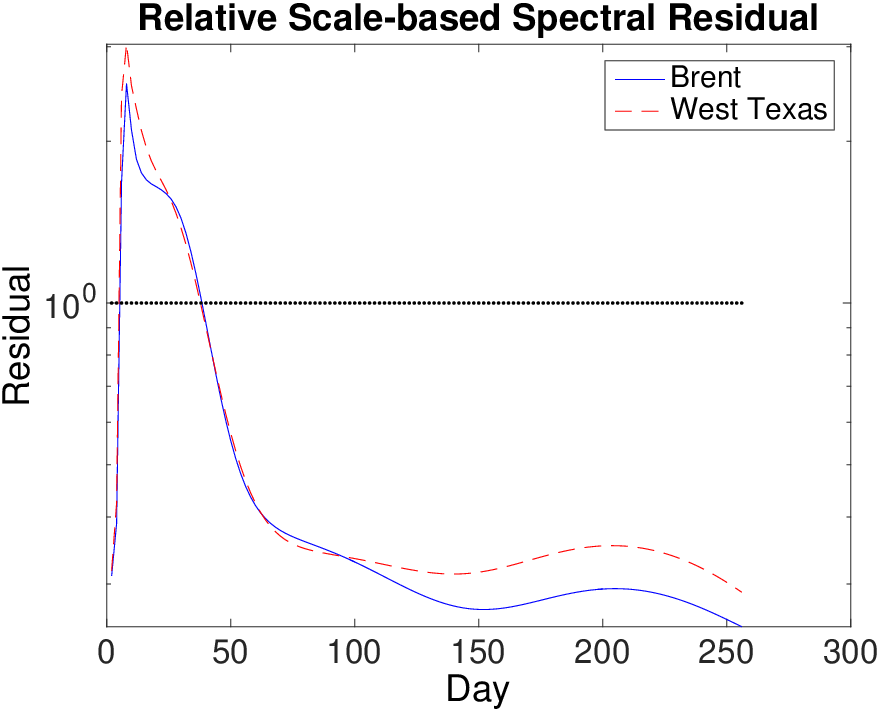
In Figure 16 we show the relative spectral residuals as a function of scale for the Brent and West Texas data sets. The relative residual is the ratio of the mean square difference between the empirical spectrum and the spectrum estimated with the robust estimator and the mean square difference between the empirical spectrum and the spectrum estimated with the ML estimator. The robust scheme shows superiority at the very short as well as at the long scales with a “spectral cross-over” at about the scale of a month, showing a more consistent tracking of the spectral behavior by the robust scheme. We seek here a robust spectral estimate for a wide-range of scales in particular for the longer scales that may be important in applications and the figure shows that for the long scales the robust estimator capture much better the spectral character.
In Figure 17 we show the actual local scale spectra by solid lines, the robust estimates by the dashed lines, and the ML estimates by the straight solid lines for two cases where the Hurst exponent estimate is high, respectively low. In the first case (top figure, West Texas) the estimates are for the robust estimator and for ML estimator. In the second case (bottom figure, Brent) the estimates are for the robust estimator and for ML estimator. We can explain the dramatic differences between the two estimates by the fact that the ML estimator is sensitive to small scales and to high-frequency noise. If the underlying process is a pure fractional Brownian motion, then the ML estimator performs very well, but if the spectrum of the process is only approximately a power law for instance, then the ML estimator may be biased.




Appendix C Further Oil Price Figures

In Figure 3 we show the scale spectra for the full period of the data while in Figure 19, the spectra correspond to the first and last 16 years of the price data (the periods 1987–2002 and 2001–2016). The strength of the price fluctuations is slightly larger in the latter half of the data for the longer scales. The qualitative behavior of the spectrum is, however, similar for the two halves of the data. The Hurst exponent associated with the two halves are for the first 16 years and for the last 16 years for the West Texas data (dashed red lines). The solid blue lines are the spectra for the Brent data set with the associated Hurst exponent estimates being and , respectively. The estimated volatilities are for the first 16 years and for the last 16 years for the West Texas data (dashed red lines). The estimated volatilities are for the first 16 years and for the last 16 years for the Brent data (solid blue lines). The straight lines in the figure are the corresponding model spectra that represent a “perfect” power law with the estimated exponents. We can observe that the spectra retain an approximate power-law behavior on very long scales. Moreover, the power law is very similar in the two halves of the data. This happens when we estimate the scale spectra over long time periods of 16 years. We show in Section 4.1 that if we consider the data over shorter subwindows, the scale spectra change over time, as we can observe vertical shifts in the spectra, corresponding to changes in the local volatility. These changes happen in a coordinated fashion for the West Texas and Brent data sets.


Appendix D Further Natural Gas Price Figures
In this section we study further the natural gas spot price and display the corresponding figures as for the crude oil price data.
In Figure 20 we plot the returns, defined as in Equation (1), for the Henry Hub natural gas data shown in Figure 10. Again the volatility of the returns process is not constant, but rather exhibits temporal variations, moreover, spikes can be seen for special market events.

Figure 21 shows the scale spectrum for the full gas data time series. The estimated Hurst exponent is and the associated volatility estimate is . The dashed red line shows the fitted scale spectrum. Note again the linear behavior corresponding to an effective “mono-fractional” behavior up to an outer scale of more than a year. The volatility is seen to be somewhat higher than for the crude price fluctuations while the Hurst exponent, and thus the price roughness, is similar. We display corresponding scale spectra in Figure 22 for respectively the first and last half of the data (the periods 1997–2007 and 2007–2016). The estimated Hurst exponents are and for the first and the last halves of the data, while the associated volatility estimates are and respectively. The qualitative behavior of the spectrum is similar for the two halves of the data.


We have calculated the spectral misfit for the natural gas data, that is root mean square of the difference of the empirical and estimated log-scale spectra as shown in Figure 6 in the case of the crude oil data. As in the case of the crude prices we observe then that the spectral misfit is low and statistically homogeneous with respect to time, which shows that the time series is well-described by the multi-fractional model with Hurst exponent and . We have moreover considered the situation when we condition on corresponding to modeling with uncorrelated returns. The estimated volatility path is then more erratic than in the multi-fractional case and the spectral residual is much larger and with stronger time coherence. Thus, again we see that the spectrum is poorly modeled by fixing as compared to the multi-fractional case.