An Issue in the Martingale Analysis of
the Influence Maximization Algorithm IMM

Influence maximization is the problem of given a social network $G=(V,E)$, a stochastic diffusion model with parameters on the network, and a budget of $k$ seeds, finding the optimal $k$ seeds $S\subseteq V$ such that the influence spread of the seeds $S$, denoted as $\sigma(S)$ and defined as the expected number of nodes activated based on diffusion model starting from $S$, is maximized. The influence maximization is originally formulated as a discrete optimization problem by Kempe et al. [13], and has been extensively studied in the literature (cf. [3] for a survey). One important direction is scalable influence maximization [6, 5, 7, 10, 12, 1, 9, 18, 17, 15], which focuses on improving the efficiency of running influence maximization algorithms on large-scale networks. The early studies on this direction are heuristics based on graph algorithms [6, 5, 7, 10, 12] or sketch-based algorithms [9]. Borgs et al. propose the novel reverse influence sampling (RIS) approach, which achieves theoretical guarantees on both the approximation ratio and near-linear expected running time [1]. The RIS approach is further improved in [18, 17, 15] to achieve scalable performance on networks with billions of nodes and edges. The IMM algorithm we discuss in this paper is from [17], which uses the martingales to improve the performance, and is considered as one of the state-of-the-art influence maximization algorithms. However, we show in this paper that the algorithm has a subtle issue that affects its correctness. The IMM algorithm has been used in later studies as a component (e.g. [19, 4, 16]), so it is worth to point out the issue and the workarounds for the correct usage of the IMM algorithm. The SSA/D-SSA algorithm of [15] is another state-of-the-art influence maximization algorithm, but the original publication also contains several analytical issues, which have been pointed out in [11].

At the core of the RIS approach is the concept of reverse-reachable (RR) sets. Given a network $G=(V,E)$ and a diffusion model, an RR set $R\subseteq V$ is sampled by first randomly selecting a node $v\in V$ and then reverse simulating the diffusion process and adding all nodes reached by the reverse simulation into $R$. Such reverse simulation can be carried out efficiently for a large class of diffusion models called the triggering model (see [13, 17] for model details). Intuitively, each node $u\in R$ if acting as a seed would activate $v$ in the corresponding forward propagation, and based on this intuition the key relationship $\sigma(S)=n\cdot\mathbb{E}[\mathbb{I}\{S\cap R\neq\emptyset\}]$ is established, where $\sigma(S)$ is the influence spread, $n=|V|$, and $\mathbb{I}$ is the indicator function. The RIS approach is to collect enough number of RR sets $\mathcal{R}=\{R_{1},R_{2},\ldots,R_{\theta}\}$, so that $\sigma(S)$ can be approximated by $\hat{\sigma}(S)=n\cdot\sum_{i=1}^{\theta}\mathbb{I}\{R_{i}\cap S\neq\emptyset\}/\theta$. We call $R_{i}\cap S\neq\emptyset$ as $S$ covering $R_{i}$. Thus, the original influence maximization problem is converted to finding $k$ seeds $S$ that can cover the most number of RR sets in $\mathcal{R}$. This is a $k$-max coverage problem, and a greedy algorithm (referred to as the NodeSelection procedure in IMM [17]) can be applied to solve it with a $1-1/e$ approximation ratio.

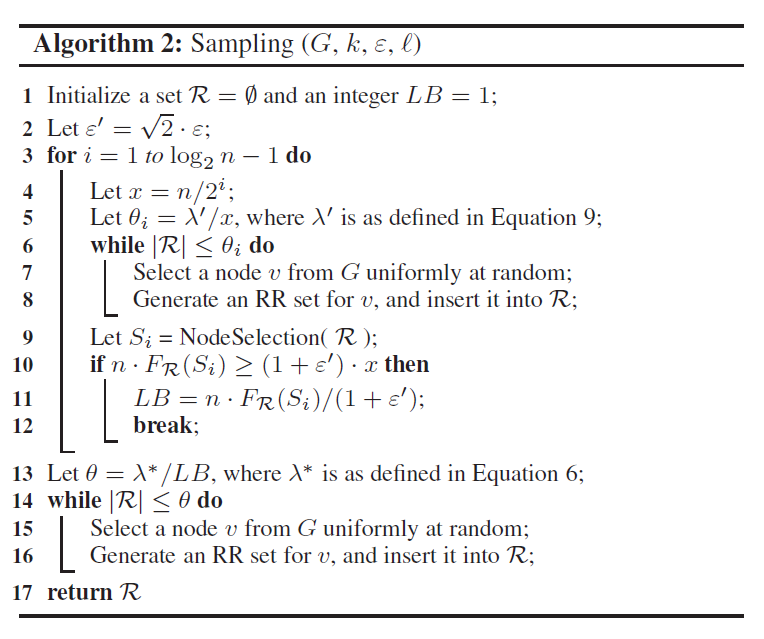
Implementations of the RIS approach differ in their estimation of the number of RR sets needed. IMM algorithm [17] iteratively doubles the number of RR sets until it obtains a reasonable estimate ${\it LB}$ as the lower bound of the optimal solution ${\it OPT}$, and then apply a formula $\theta=\lambda^{*}/{\it LB}$, where $\lambda^{*}$ is a constant dependent on the problem instance, to get the final number of RR sets needed (See Fig. 1 for the reprint of the Sampling procedure of IMM).

The main issue of the IMM analysis in [17] is at its correctness claim of Theorem 4, which shows that the output of IMM gives a $1-1/e-\varepsilon$ approximate solution with probability at least $1-1/n^{\ell}$. The proof of this part is very brief, containing only one sentence as excerpted below, which combines the result from Theorem 1 and Theorem 2.

“By combining Theorems 1 and 2, we obtain that Algorithm 3 returns a $(1-1/e-\varepsilon)$-approximate solution with at least $1-1/n^{\ell}$ (probability).”

At the high level, Theorem 1 claims that if NodeSelection procedure is fed with an RR set sequence of length at least $\theta\geq\lambda^{*}/{\it OPT}$, then with probability at least $1-1/n^{\ell}$, NodeSelection outputs a seed set that is a $1-1/e-\varepsilon$ approximate solution. Then Theorem 2 claims that the Sampling procedure outputs an RR set sequence of length at least $\lambda^{*}/{\it OPT}$ with probability at least $1-1/n^{\ell}$. It may appear that we could use a simple union bound to combine the two theorems to show that IMM achieves the $1-1/e-\varepsilon$ approximation with probability at least $1-2/n^{\ell}$. Finally, we just need to reset $\ell=\ell+\log 2/\log n$ to change the probability from $1-2/n^{\ell}$ to $1-1/n^{\ell}$.¹¹ 1 The original paper has a typo here. It says to reset $\ell$ to $\ell(1+\log 2/\log n)$, but this is not necessary. Only resetting $\ell$ to $\ell+\log 2/\log n$ is enough.

However, with a closer inspection, Theorem 1 is true only for each fixed length $\theta\geq\lambda^{*}/{\it OPT}$, but the Sampling procedure returns an RR set sequence of random length. Henceforth, to make the distinction explicit, we use $\tilde{\theta}$ to denote the random length returned by the Sampling procedure. Technically, this $\tilde{\theta}$ is a stopping time, a concept frequently used in martingale processes [14]. Thus, what Theorem 2 actually claims is $\Pr\{\tilde{\theta}\geq\lambda^{*}/{\it OPT}\}\geq 1-1/n^{\ell}$. Due to this discrepancy between fixed length and random length in RR set sequences, we cannot directly combine Theorem 1 and Theorem 2 to obtain Theorem 4 as in the paper. This is the main issue of the analysis in the IMM paper [17].

In the next two subsections, we will provide more detailed discussion to illustrate the above issue. In Section 2.3, we first make it explicit what is the exact probability space we use for the analysis of the IMM algorithm. Then in Section 2.4, we go through lemma by lemma on the original analysis to make the distinction between the fixed length $\theta$ and the random stopping time $\tilde{\theta}$ explicit, so that the issue summarized above is more clearly illustrated.

For the following discussion, we will frequently refer to certain details in the Sampling procedure of IMM, namely Algorithm 2 of IMM in [17] (see Fig. 1).

To clearly understand the random stopping time $\tilde{\theta}$, we first clarify the probability space upon which $\tilde{\theta}$ is defined. We first note that from the algorithm, the maximum possible number of RR sets the algorithm could generate is $\lceil\lambda^{*}\rceil$ (defined in Eq.(6)). Thus we view the probability space as the space of all $\lceil\lambda^{*}\rceil$ RR set sequences $R_{1},R_{2},\ldots,R_{\lceil\lambda^{*}\rceil}$, where each $R_{i}$ is generated i.i.d. We denote this space as $\Omega$. Then in one run of the IMM algorithm, one such RR set sequence $\mathcal{R}_{0}$ is drawn from the probability space $\Omega$. In the $i$-th iteration of the Sampling procedure, the algorithm gets the prefix of the first $\theta_{i}$ ($\theta_{i}$ is defined in line 5 of Algorithm 2) RR sets in the above sequence $\mathcal{R}_{0}$, and based on certain condition about this prefix the algorithm decides whether to continue the iteration or stop; and when it stops, it determines the final number $\tilde{\theta}=\lambda^{*}/{\it LB}$ of RR sets needed, and retrieves the prefix of $\tilde{\theta}$ RR sets from $\mathcal{R}_{0}$. Note that $\tilde{\theta}$ here is the $\theta$ used in line 13 of Algorithm 2, but we explicitly use $\tilde{\theta}$ to denote that it is a random variable (because ${\it LB}$ is a random variable), and its value is determined by the prefix of RR sets in $R_{1},R_{2},\ldots$. In contrast, for a fixed $\theta$ such as the $\theta$ used in Theorem 1, it simply corresponds to the $\theta$ RR sets in the sequence sample $\mathcal{R}_{0}$. For convenience, we use $\mathcal{R}_{0}[\theta]$ to denote the prefix of $\mathcal{R}_{0}$ of fixed length $\theta$, and $\Omega[\theta]$ to be the subspace of all RR set sequences of length $\theta$. Note that we use $\Omega$ and $\Omega[\theta]$ to refer to both the set of sequences and their distribution.

Hopefully we clarify the distinction between the fixed-length sequence $R_{1},R_{2}$, $\ldots,R_{\theta}$ and the actual sequence $R_{1},R_{2},\ldots,R_{\tilde{\theta}}$ generated by the sampling phase with a random stopping time $\tilde{\theta}$. We now revisit the technical lemmas and the theorems of the paper to explicitly distinguish between the usage of fixed length $\theta$ and random length $\tilde{\theta}$.

First and foremost, the martingale inequalities summarized in Corollaries 1 and 2 should only work for a fixed constant $\theta$, not for a random stopping time, because they come from standard martingale inequalities as summarized in [8], which deals with martingales of fixed length. However, the authors introduce these inequalities in the context of RR set sequence generated by the Sampling procedure (see the first sentence in Section 3.1 of [17]). As we explained, the RR set sequence generated by the Sampling procedure has random length $\tilde{\theta}$, so Corollaries 1 and 2 should not be applied to such random length sequences. This is the source of confusion leading to the incorrectness of the proof of Theorem 4. Henceforth, we should clearly remember that Corollaries 1 and 2 only work for fixed length $\theta$.

Next, for Lemmas 3 and 4, the $\theta$ there should refer to a fixed number, because their proofs rely on the martingale inequalities in Corollary 1 and 2, which are correct only for a fixed $\theta$.

For Theorem 1, same as discussed above, if we view $\theta$ as a fixed constant, then Theorem 1 is correct. We need to remark here that Theorem 1 talks about the node selection phase, so its exact meaning is that if we feed the NodeSelection procedure with an RR set sequence of fixed length $\theta$, randomly drawn from the space $\Omega[\theta]$, then the node selection phase would return an approximate solution. Therefore, it is not applicable when the NodeSelection procedure is fed with the RR set sequence generated from the Sampling procedure, since this sequence has a random length and is not drawn from the space $\Omega[\theta]$ for a fixed $\theta$.

Lemma 5 and Corollary 3 are still correct, since they are not related to the application of martingale inequality. For Lemmas 6 and 7, again they are correct when $\theta$ is a fixed number satisfying inequality (8).

For Theorem 2, as already mentioned in Section 2.2, it is about the RR set sequence $\mathcal{R}=\{R_{1},R_{2},\ldots,R_{\tilde{\theta}}\}$ generated by the Sampling procedure, with random length $\tilde{\theta}$, and its technical claim is

where the probability is taken from the probability space $\Omega$, the random sample $\mathcal{R}_{0}$ of which determines the actual random length of output $\tilde{\theta}$. The proof of Theorem 2 uses Lemma 6 and Lemma 7. When it uses Lemma 6 and Lemma 7, it is in the context of the Sampling procedure, and the $\theta$ used for Lemma 6 and Lemma 7 in this context is exactly the $\theta_{i}=\lambda^{\prime}/x_{i}$ defined in line 5 of algorithm, where $\lambda^{\prime}$ is a constant defined in Eq.(9), and $x_{i}=n/2^{i}$, and $i$ refers to the $i$-th iteration in the Sampling procedure. Therefore, $\theta_{i}$ indeed is a constant that does not depend on the generated RR sets, and the applications of Lemmas 6 and 7 is in general appropriate. However, the original proof of Theorem 2 is brief, and there is a subtle point that may not be clear from the proof, and thus some extra clarification is deserved here.

The subtlety is that, Lemmas 6 and 7 are correct when the NodeSelection procedure is fed with a fixed length RR set sequence sampled from $\Omega[\theta]$. However, in the $i$-th iteration of the Sampling procedure, the actual RR set sequence fed into NodeSelection is not sampled from the space $\Omega[\theta_{i}]$. This is because the fact that the algorithm enters the $i$-th iteration implies that the previous RR set sequence failed the coverage condition check in line 10 in the previous iterations, and thus the actual sequence fed into NodeSelection in the $i$-th iteration is a biased sample. This subtlety makes the rigorous proof of Theorem 2 longer, but does not invalidate the Theorem. Intuitively, for a random sample $\mathcal{R}_{0}[\theta_{i}]$ drawn from $\Omega[\theta_{i}]$, even if $\mathcal{R}_{0}[\theta_{i}]$ would not make the algorithm survive to the $i$-th iteration, we could still treat it as if it is fed to NodeSelection in the $i$-th iteration, and use Lemmas 6 and 7 to argue that some event $\mathcal{E}_{i}$ only occurs with a small probability $\delta_{3}$. Then the event that both algorithm enters the $i$-th iteration and $\mathcal{E}_{i}$ occurs must be also smaller than $\delta_{3}$. For completeness, in the appendix, we provide a more rigorous technical proof of Theorem 2 applying the above idea.

Continuing to Lemmas 8 and 9, similar to Lemma 6 and Lemma 7, it is correct when we treat $\theta$ as a constant. For Lemma 9, it uses Lemma 8, and if we treat the application of Lemma 8 in the same way as we treat the application of Lemmas 6 and 7 in the proof of Theorem 2, then Lemma 9 is correct. Lemma 10 and Theorem 3 are independent of the application of martingale inequalities and are correct.

Finally, we investigate the proof of Theorem 4, in particular the part on the correctness of the IMM algorithm. As outlined in Section 2.2, a direct combination of Theorem 1 and Theorem 2 is problematic. We now discuss this point with more technical details.

For Theorem 1, based on our above discussion, it works for a fixed value of $\theta$. More precisely, when we use the setting discussed after Theorem 1, what it really says is that, for all fixed $\theta\geq\lambda^{*}/{\it OPT}$, if we use a random sample $\mathcal{R}_{0}[\theta]$ drawn from distribution $\Omega[\theta]$, then when we feed the NodeSelection procedure with $\mathcal{R}_{0}[\theta]$, the probability that NodeSelection returns a seed set that is a $(1-1/e-\varepsilon)$ approximate solution is at least $1-1/n^{\ell}$. To make it more explicit, let $S^{*}_{k}(\mathcal{R})$ be the seed set returned by NodeSelection under input RR set sequence $\mathcal{R}$. Let $Y(S)$ be an indicator, and it is $1$ when seed set $S$ is a $(1-1/e-\varepsilon)$ approximate solution, and it is $0$ otherwise. Then, what Theorem 1 says is,

Next, as discussed above, what Theorem 2 really says is given in Eq. (1). Also to make it more precise and use the same base sample from the probability space, let $\mathcal{R}_{0}$ be the sample drawn from $\Omega$, and let $\mathcal{R}(\mathcal{R}_{0})=\{R_{1},R_{2},\ldots,R_{\tilde{\theta}}\}$ be the sequence generated by the Sampling procedure, and $\tilde{\theta}(\mathcal{R}_{0})$ denote its length. Thus by definition, $\mathcal{R}(\mathcal{R}_{0})$ is the first $\tilde{\theta}(\mathcal{R}_{0})$ RR sets of $\mathcal{R}_{0}$. Then Theorem 2 (and Eq. (1)) is restated as

For Theorem 4, we want to bound the probability that using the Sampling procedure output $\mathcal{R}(\mathcal{R}_{0})$ to feed into NodeSelection, its output fails to provide the $1-1/e-\varepsilon$ approximation ratio, that is,

The following derivation further separates the left-hand side of Eq. (4) into two parts by the union bound:

where the last inequality is by Theorem 2 (Eq. (3)). To continue, we want to bound

However, the above inequality is incompatible with Inequality (2), because Inequality (2) holds for each fixed $\theta\geq\frac{\lambda^{*}}{{\it OPT}}$, but Inequality (6) is for all $\tilde{\theta}(\mathcal{R}_{0})\geq\frac{\lambda^{*}}{{\it OPT}}$. This is where the direct combination of Theorem 1 and Theorem 2 would fail to produce the correctness part of Theorem 4.

One simple workaround is that in the IMM algorithm, after determining the final length $\tilde{\theta}$ of the RR set sequence, regenerate the entire RR set sequence of length $\tilde{\theta}$ from scratch, and use the newly generated sequence as the output of the Sampling algorithm and feed it into the final call to NodeSelection. That is, after line 13 of Algorithm 2, regenerate $\tilde{\theta}$ RR sets instead of lines 14-16.

Intuitively, this would feed the final call of NodeSelection with an unbiased RR set sequence so that Theorem 1 can be applied. We represent this new unbiased sequence as a new independent sample $\mathcal{R}^{\prime}_{0}$ from the probability space $\Omega$, and then taking the prefix of $\mathcal{R}^{\prime}_{0}$ with $\tilde{\theta}(\mathcal{R}_{0})$ RR sets, where $\tilde{\theta}(\mathcal{R}_{0})$ is the number of RR sets determined from sequence $\mathcal{R}_{0}$ that is needed for the final call of NodeSelection. Thus we use the notation $\mathcal{R}^{\prime}_{0}[\tilde{\theta}(\mathcal{R}_{0})]$ to represent the RR set sequence that is fed into the final call of NodeSelection. The correctness can be rigorously proved as follows. First, Eq. (4) for Theorem 4 is changed to:

To show the above inequality, following a similar derivation as in Eq. (5), what we need to show is the following instead of Eq. (6):

This can be achieved by the following derivation:

The key step is Eq. (9), where because $\mathcal{R}^{\prime}_{0}$ is independent of $\mathcal{R}_{0}$ (we regenerate a new RR set sequence for the last call to NodeSelection), we can represent the probability $\Pr_{\mathcal{R}_{0}\sim\Omega,\mathcal{R}^{\prime}_{0}\sim\Omega}\left\{\tilde{\theta}(\mathcal{R}_{0})=\theta\wedge Y(S^{*}_{k}(\mathcal{R}^{\prime}_{0}[\theta]))=0\right\}$ as the product of two separate factors. Therefore, the correctness part of Theorem 4 now holds. Note that within the Sampling procedure, we do not need to regenerate RR set sequences from scratch (before line 9 of Algorithm 2), because by our detailed discussion in Section 2.4, even without regenerating RR sets, Theorem 2 still holds with a more careful argument.

In terms of the running time, this workaround at most doubles the number of RR sets generated, and thus its running time only adds a multiplicative factor of $2$ to the original result. Therefore, the asymptotic running time remains as $O((k+\ell)(n+m)\log n/\varepsilon^{2})$ in expectation.

The second workaround is by directly bounding Eq. (6) by a union bound, as shown in the derivation below.

Comparing the above derivation with the similar one for workaround 1, the key difference is between Eq. (9) and Eq. (10). In Eq. (9), we could keep $\Pr_{\mathcal{R}_{0}\sim\Omega}\{\tilde{\theta}(\mathcal{R}_{0})=\theta\}$ because the event $\{\tilde{\theta}(\mathcal{R}_{0})=\theta\}$ is independent of the event $\{Y(S^{*}_{k}(\mathcal{R}^{\prime}_{0}[\theta]))=0\}$ in the second term. But in Eq. (10), we cannot extract $\Pr_{\mathcal{R}_{0}\sim\Omega}\{\tilde{\theta}(\mathcal{R}_{0})=\theta\}$ because the event $\{\tilde{\theta}(\mathcal{R}_{0})=\theta\}$ is correlated with the event $\{Y(S^{*}_{k}(\mathcal{R}_{0}[\theta]))=0\}$ in the second term. Thus we have to simply drop the event $\{\tilde{\theta}(\mathcal{R}_{0})=\theta\}$, causing the bound to be inflated by a factor of $\lceil\lambda^{*}\rceil$.

Using Inequality (12), our second workaround is to enlarge $\ell$ to $\ell^{\prime}$ so that $\lceil\lambda^{*}\rceil/n^{\ell^{\prime}}\leq 1/n^{\ell}$. However, $\lambda^{*}$ is also dependent on $\ell$. To make it clear, we write it as $\lambda^{*}(\ell)$. What we want is to set $\ell^{\prime}=\ell+\gamma$, such that

This means we want $\lceil\lambda^{*}(\ell+\gamma)\rceil\leq n^{\gamma}$. From Eqs.(5) and (6) in [17], we have

where the relaxation in the inequality above is loose, involving relaxing the first square root term to the second one, relaxing $(1-1/e)$ to $1$, relaxing $\binom{n}{k}$ to $n^{k}$, relaxing $\log 2$ to $\log n$, and thus the $-1$ above can be certainly compensated by the relaxation, and it is used for relaxing the $\lceil\lambda^{*}(\ell+\gamma)\rceil$ next. Thus, to achieve $\lceil\lambda^{*}(\ell+\gamma)\rceil\leq n^{\gamma}$, we just need $8n(k+\ell+\gamma+1)\log n\cdot\varepsilon^{-2}\leq n^{\gamma}$. Asymptotically, $\gamma>1$ would be fine for large enough $n$. For a conservative bound, it is very reasonable to assume that $\varepsilon^{-1}\leq n$, $k+\ell+\gamma+1\leq n$, then we just need $8\log n\leq n^{\gamma-4}$, which means setting $\gamma\geq 4+\log(8\log n)/\log n$ is enough. Thus $\gamma$ is essentially a small constant.

In practice, $\gamma$ could be computed by a binary search once the parameters $n$, $k$, $\ell$ and $\varepsilon$ of the problem instance are given. Then we can set $\ell=\ell+\log 2/\log n+\gamma$ in the algorithm. By increasing $\ell$ with a small constant $\gamma$ (e.g. $\gamma=2.5$), the running time increases from $O(k+\ell)(m+n)\log n/\varepsilon^{2})$ to $O(k+\ell+\gamma)(m+n)\log n/\varepsilon^{2})$, so the running time penalty is likely to be smaller than that of the first workaround. Our experimental results below validate this point.

We evaluate the two workarounds and compare them against the original IMM algorithm on two real world datasets: (a) NetHEPT, a coauthorship network with 15233 nodes and 31373 edges, mined from arxiv.org high energy physics section, and (b) DBLP, another coauthorship network with 655K nodes and 1990K edges, mined from dblp.uni-trier.de. We use independent cascade model with edge probabilities set by the weighted cascade method [13]: edge $(u,v)$’s probability is $1/d_{v}$ where $d_{v}$ is the in-degree of $v$. These datasets are frequently used in other influence maximization studies such as [5, 17, 4].

We use IMM, IMM-W1, and IMM-W2 to denote the original IMM, the IMM with the first and the second workarounds, respectively. For IMM-W2, we use binary search to find an estimate of $\gamma$ satisfying $\lceil\lambda^{*}(\ell+\gamma)\rceil\leq n^{\gamma}$. We set parameters $\varepsilon=0.1$, $\ell=1$, and influence spread is the average of $10000$ simulation runs. We test the algorithms in seed set sizes $k=50,100,\ldots,500$. The code is written in C++ and compiled by Visual Studio 2013, and is run on a Surface Pro 4 with dual core 2.20GHz CPU and 16GB memory.

The influence spread and running time results are shown in Figure 2. As expected, all three algorithms achieve indistinguishable influence spread, since the two workarounds are to fix the theoretical issue on the dependency of RR sets, and should not affect much on the actual performance of the IMM algorithm. In terms of running time, also as expected, IMM-W1 has the worst running time, but is within twice of running time of the IMM algorithm. IMM-W2 has much closer running time to IMM, though is still in general slower. We further observe that the $\gamma$ value used for IMM-W2 is within $2.5$ for the NetHEPT dataset and within $2$ for the DBLP dataset. Therefore, it looks like that we can use the second workaround to provide a rigorous theoretical guarantee while achieving similar running time as the original IMM.

References

- [1] Christian Borgs, Michael Brautbar, Jennifer Chayes, and Brendan Lucier. Maximizing social influence in nearly optimal time. In SODA, 2014.
- [2] Wei Chen. An issue in the martingale analysis of the influence maximization algorithm IMM. Technical Report arXiv:1808.09363, 2018.
- [3] Wei Chen, Laks VS Lakshmanan, and Carlos Castillo. Information and Influence Propagation in Social Networks. Morgan & Claypool Publishers, 2013.
- [4] Wei Chen and Shang-Hua Teng. Interplay between social influence and network centrality: A comparative study on shapley centrality and single-node-influence centrality. In WWW, pages 967–976, 2017.
- [5] Wei Chen, Chi Wang, and Yajun Wang. Scalable influence maximization for prevalent viral marketing in large-scale social networks. In KDD, 2010.
- [6] Wei Chen, Yajun Wang, and Siyu Yang. Efficient influence maximization in social networks. In KDD, 2009.
- [7] Wei Chen, Yifei Yuan, and Li Zhang. Scalable influence maximization in social networks under the linear threshold model. In ICDM, 2010.
- [8] Fan Chung and Linyuan Lu. Concentration inequalities and martingale inequalities: A survey. Internet Mathematics, 3(1):79–127, 2006.
- [9] Edith Cohen, Daniel Delling, Thomas Pajor, and Renato F. Werneck. Sketch-based influence maximization and computation: Scaling up with guarantees. In CIKM, pages 629–638, 2014.
- [10] Amit Goyal, Wei Lu, and Laks V. S. Lakshmanan. SIMPATH: An Efficient Algorithm for Influence Maximization under the Linear Threshold Model. In ICDM, 2011.
- [11] Keke Huang, Sibo Wang, Glenn S. Bevilacqua, Xiaokui Xiao, and Laks V. S. Lakshmanan. Revisiting the stop-and-stare algorithms for influence maximization. PVLDB, 10(9):913–924, 2017.
- [12] Kyomin Jung, Wooram Heo, and Wei Chen. IRIE: Scalable and Robust Influence Maximization in Social Networks. In ICDM, 2012.
- [13] David Kempe, Jon M. Kleinberg, and Éva Tardos. Maximizing the spread of influence through a social network. In KDD, 2003.
- [14] Michael Mitzenmacher and Eli Upfal. Probability and Computing. Cambridge University Press, 2005.
- [15] Hung T. Nguyen, My T. Thai, and Thang N. Dinh. Stop-and-stare: Optimal sampling algorithms for viral marketing in billion-scale networks. In SIGMOD, pages 695–710, 2016.
- [16] Lichao Sun, Weiran Huang, Philip Yu, and Wei Chen. Multi-round influence maximization. In KDD, 2018.
- [17] Youze Tang, Yanchen Shi, and Xiaokui Xiao. Influence maximization in near-linear time: a martingale approach. In SIGMOD, 2015.
- [18] Youze Tang, Xiaokui Xiao, and Yanchen Shi. Influence maximization: near-optimal time complexity meets practical efficiency. In SIGMOD, 2014.
- [19] Yu Yang, Xiangbo Mao, Jian Pei, and Xiaofei He. Continuous influence maximization: What discounts should we offer to social network users? In SIGMOD, 2016.
Appendix
Appendix A Detailed Proof of Theorem 2 in [17]
In this appendix, we provide a detailed re-proof of Theorem 2 in [17]. The proof follows the idea outlined in Section 2.4, and is meant to make the original proof of Theorem 2 in [17] more rigorous and eliminate possible ambiguities on handling the martingale sequence dependency in the original proof.
Detailed Proof of Theorem 2.
Let for , and . Let be the index such that . Let , where is defined in Eq.(9) of [17]. For a generic RR set sequence , we use to denote the output of the NodeSelection procedure with input . Let denote the full same RR set sequence from the probability space that corresponds to a run of the IMM algorithm. Note that the appearing in lines 9 and 10 is the prefix of with length , so we use expression explicitly to replace in these lines. This means the output in line 9 should be written as . Define event , which corresponds to the condition in line 10. Note that only when are false, the Sampling procedure would enter the -th iteration, and would check the condition in line 10 corresponding to the even . Let be the lower bound computed in line 11, just before the Algorithm 2 breaks the for-loop.
To prove Theorem 2 (or equivalent Eq. (1)), by line 13 of Algorithm 2, it is sufficient to show that with low probability . The way to show this is by showing that for each round , only with a low probability the algorithm breaks out of the for-loop in the -th iteration; and if the algorithm breaks out of the for-loop at least in the -th iteration or above, with a low probability, . Formally, we have