Embryonic lateral inhibition as optical modes: an analytical framework for mesoscopic pattern formation
Abstract
Cellular checkerboard patterns are observed at many developmental stages of embryos. We study an analytically tractable model for lateral inhibition and show that a coupling coefficient with a negative value is sufficient to obtain noisy or periodic checkerboard patterns. We solve the case of a linear chain of cells explicitly and show that noisy anti-correlated patterns are available in a post-critical regime . In the sub-critical regime a periodic and alternating steady state is available, where pattern selection is determined by making an analogy with the optical modes of phonons. For cells arranged in a hexagonal lattice, the sub-critical pattern can be driven into three different states: two of those states are periodic checkerboards and a third in which both periodic states coexist.
pacs
Valid PACS appear hereIntroduction.- Pattern formation in living tissue is an emergent property that arises from cell signaling. In his seminal work Alan Turing proposed that the anatomical structure of an embryo is determined by self-organised chemical patterns [1]. In his theory the interplay between reactions and diffusion of two chemical species give rise to self-organized periodic structures. Although this model is difficult to implement in practice with the restrictions proposed by Turing [2, 3], variants of this model system have been extensively studied theoretically [4] and have been successfully used to describe the patterns of living systems at the tissue level [5, 6, 7].
There is a subclass of patterns in living systems where the characteristic length scale is the size of a single cell (figure 1 a). These are fine-grained patterns where the protein expression levels vary abruptly and regularly between cells, reminiscent of checkerboards (figure 1 a). In this case the reaction-diffusion mechanism from Turing cannot describe their formation, as its characteristic length scale corresponds to a wavenumber equal to infinity in a continuum description. These patterns appear in several examples of cellular tissues such as in the arrangement of photo receptor cells in the eye [8], sensory hair cells in the auditory epithelium [9, 10], and sensory bristles in the fly thorax [11] among others. Lateral inhibition has been proposed as a basic mechanism whereby a cell inhibits the expression levels of a protein in its neighbouring cells. The Delta-Notch signaling system is a pathway frequently used by different species to create these fine-grained tissue patterns [12].
Collier et al. [13] pioneered theoretical work in lateral inhibition, analysing a spatially discrete model for Delta-Notch signaling that reproduced periodic and fine-grained patterns. Since then, extensions of this model (or similar ones) have incorporated different effects observed in experiment, such as self regulation (cis-interactions) [14], state dependent coupling strength [15], time delay in signaling [16, 17] and cis-interactions with time delay [18]. These models are difficult to analyse analytically and they rely on numerical simulations to determine how patterns emerge. In this work we propose a generic model for lateral inhibition that is analytically tractable, allowing us to understand pattern selection for this class of systems. The model consists of the following equation

| (1) |
where the state of each cell placed in a lattice is represented by the variable . The model describes the effects of cis-interactions where is an internal component that influences the production of and is the strength of nonlinear degradation. The cells are influenced by the state of their nearest neighbours (trans-regulation) with coupling strength (figure 1 b).
In this work we determine the conditions necessary to obtain noisy anticorrelated patterns and periodic alternating patterns for given the signaling strength and the profile of the internal production rate . These lateral inhibition patterns appear only when the value of is negative. If we set in equation (1), there is a sub-critical regime where the uniform state is unstable and a post-critical regime where is stable. In the sub-critical regime we consider a spatially uniform profile for while in post-critical regime we consider spatially uncorrelated and time-constant values of .
The case of a one dimensional chain of cells is explicitly solved, and these results helps us to analyse the case of cells placed in an hexagonal lattice (figure 1 c). By making an analogy to lattice (phonon) vibrations from solid state physics [19], we determine a potential function that determines the possible sub-critical states of the system. In cells arranged in an hexagonal lattice, these states lie on a periodic lattice (blue points in figure 1 c), where given we obtain: 1) a periodic pattern filled with the basis structure denoted (figure 1 d), 2) a pattern filled with the basis (figure 1 d), or 3) a state where both basis and coexist.
Linear reponse of a chain of cells.- We consider a one dimensional chain of cells signaling each other following Equation (1). For this example, we define a cell in the middle of the chain with index . First consider the linearized version of Equation (1) around , which is given by
| (2) |
As a first step to charaterize its dynamics we study the linear response function of the chain to the static input , where corresponds to the Kronecker delta. The linear response of an infinite chain is given by the following expression
| (3) |
(see supplement for details [20]). Note in equation (3) there is a term proportional to , therefore if the values of alternate between positive and negative values (figure 2 a, lateral inhibition), while for the values of decay smoothly (figure 2 b, lateral induction).
We next calculate the correlations in a chain of now considering an stochastic input characterized by
| (4) |
The linear response function is used to calculate the correlation between nearest neighbors [20], which is given by

| (5) |
The correlations are zero for and they diverge to for , this is the same value found in Collier et al. [13] by linear stability analysis. The divergence in the correlation coefficient is characteristic of a critical point [21], while its negative sign denotes that the neighbors are anti-correlated. At this critical point the uniform state becomes unstable. There is good agreement between numerical and the analytical approximation given by Equation (5) (see Figure 2 c). Examples of anti-correlated noisy patterns in Figure 2 (d) show that as decreases, the probability of having alternating neighbours increases.
Analogy to optical modes.- The results shown in Figure 2 (a) and (b) are reminiscent of the optical and acoustic modes of phonons from solid state physics [19]. Phonons are vibrations in a periodic crystal. The crystal is composed by a set of lattice sites, where at each site there is a molecule with several atoms called the basis (also termed as the crystal unit cell). If the basis is diatomic, two vibration modes are allowed. In the optical mode the position of atoms alternate between positive and negative values between neighbors, and in the acoustic mode this alternation does not happen [19]. The linear response of for (figure 2 a) is analogous to the optical mode and for to the acoustic mode (figure 2 b).
This analogy to the optical modes is useful to analyze the sub-critical state . We start by setting a uniform in equation (1). We divide the chain of into lattice sites and at each site there is a basis with two components and . The components corresponds to with and even values of , and the remainder corresponds to (figure 3 a). In this notation equation (1) for the one dimensional chain becomes
| (6) |
| (7) |
| (8) |
| (9) |
where corresponds to the position in the line tissue and is the distance between the lattice points. Assuming a uniform stationary state for both and then we define a potential
| (10) |

for this is a double well potential (figure 3 b). One minimum of this potential we denote as the state where and . The other minimum we denote as where and . From this potential we expect that the steady states of Equation (1) consists of anti-correlated neighbors. We test this prediction with a numerical simulation of equation (1). We set and the uniform initial condition to (figure 3 (c) at ). This initial state is unstable and the values decrease towards (). A wave emerges from the edges of the chain and travels towards the center, reminiscent of waves observed in the Collier model [22]. The values of intercalate between values close to , in this regime . At long times the pattern remains in this alternating state (figure 3 (c) at ). Thus there is agreement between the predictions of the potential and the steady state of the system.

Cells in an hexagonal lattice.- Typical fine-grained pattern formation occurs in epithelial tissues, single layers of cells. As a good approximation of these tissues, we analyze the case of cells placed in an hexagonal lattice. Using the observations of a linear chain of cells we analyze the response to a random input in epithelial tissues. Figure 4 shows the projection , where corresponds to the Heaviside theta, for different steady states as a function . As in the example of the previous section, we see that the likelihood of being surrounded by anti-correlated neighbors increases as the value of decreases.
We proceed by analyzing the sub-critical regime of equation (1) by dividing into different components as in the previous example. Again we consider a spatially uniform . Defining a basis with two variables as in the linear chain, and rewriting Equation (1) we notice that the interactions are asymmetric [20]. Therefore we rewrite Equation (1) in terms of an hexagonal lattice with lattice sites (see figure 1 c) and place at each lattice site a basis with three components , and . We derive a potential well for this case [20].
| (11) |
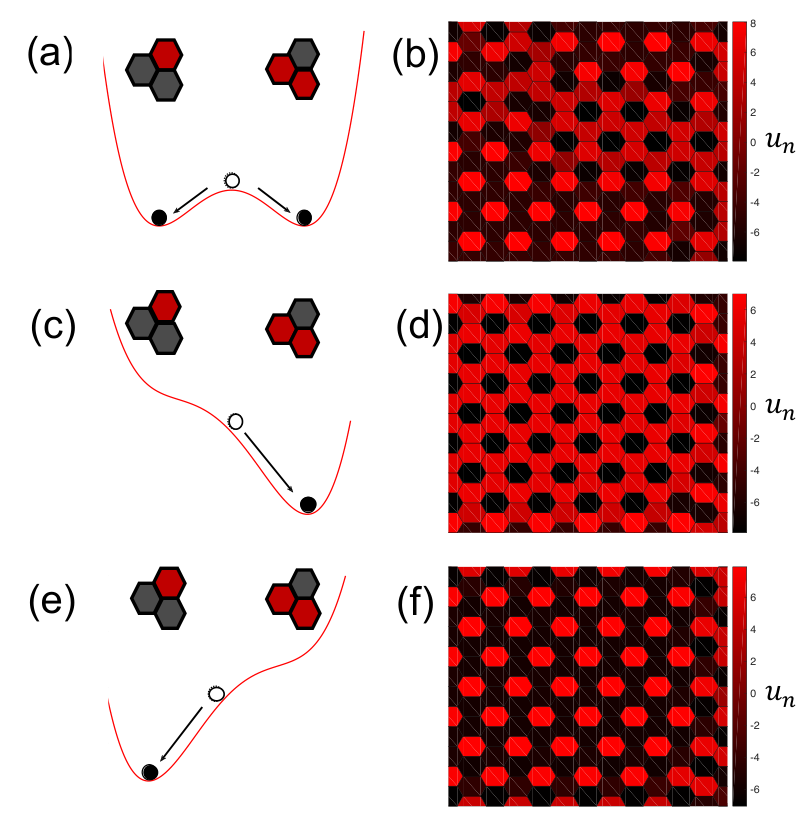
The state of the tissue becomes unstable at [13], in this case we find the minima of this potential and their stability numerically. Figure 5 shows the position of the stable (black points) and the metastable states (white points) projected onto the axis from the potential given by equation (11), as a function of for [20]. When there are six stable states, three correspond to the basis (figure 5 a) mentioned in the introduction (see figure 1 d). The other stable states corresponds to the basis . A simplified picture of this potential is shown in Figure 6 (a) as a double well potential where each minima corresponds to a base. In figure 6 (b) we show a numerical simulation of Equation (1) in this regime initiated from uniform initial conditions. The final pattern has two coexisting regions, one filled with the basis and the other filled with .
If we increase further the value of (figure 5 b), the points indicating the metastable states move closer to the points indicating the basis . After crossing a critical value for , the stable points corresponding to disappear by colliding with a metastable point. In the simplified picture shown in Figure 6 by increasing the parameter the double well potential (Figure 6 a) becomes a single well potential (Figure 6 c). The single minima corresponds to the basis . Numerical simulations in this regime results in a pattern filled with the basis (figure 6 d). If we repeat the same procedure as before but decreasing the control parameter , then the potential has a single well with the minima corresponding to (figure 6 e). Simulations in this regime shows a pattern filled with (figure 6 f). We note that some final patterns can contain defects depending on initial conditions [20].
Conclusions.- In this work we have proposed an analytically tractable model for lateral inhibition. We have shown how fine-grained checkerboard patterns depend on the model parameters. By making an analogy with optical modes from lattice phonons we are able to determine how fine-grained patterns are selected. Thus our model is a generic description of lateral inhibition that explains the transitions observed in more detailed models as the ones in [13, 14, 15, 16, 17, 18].
Our model brings a new framework to studying and understanding pattern selection in both natural and synthetic biological fine-grained systems. Particularly attractive experimental scenarios for testing these ideas are in vitro cellular systems with synthetic intercellular signaling pathways such as recently reported by Matsuda et al [23]. Disrupting Delta-Notch communication between cells in this system using a chemical inhibitor yielded a uniform expression of Delta across the tissue. Removal of the inhibitor allowed Delta-Notch signaling to initiate and caused the evolution of a fine-grained pattern of Delta expression. This mimics our model’s behaviour when the coupling strength is modulated from to . This and similar experimental systems [24, 25] also raise the possibility of controlling the initial expression levels of Delta, or an equivalent signal, which would be analogous to modulating in the model.
Finally, our analysis shows that pattern formation by cell signalling has two regimes. A regime where the steady state is composed by acoustic modes, this is the reaction-diffusion regime scenario proposed by Turing, and a regime composed by optical modes that corresponds to the fine-grained patterns of lateral inhibition.
Acknowledgements.- We would like to thank Marta Ibañes and José M. Sancho for sharing their unpublished manuscript with a similar model. Their analysis and observations are complementary to our work.
References
- [1] A. Turing, Philos. Trans. Royal Soc. B 237, 37 (1952).
- [2] V. Castets, E. Dulos, J. Boissonade, and P. D. Kepper, Phys. Rev. Lett. 64, 2953 (1990).
- [3] Q. Ouyang and H. Swinney, Nature 352, 610 (1991).
- [4] M. Cross and H. Greenside, Pattern Formation and Dynamics in Nonequilibrium Systems (Cambridge University Press, 2009).
- [5] S. Kondo and R. Asai, Nature 376, 765 (1991).
- [6] M. Yamaguchi, E. Yoshimoto, and S. Kondo, Proc. Nat. Acad. Sci. 12, 4790 (2007).
- [7] J. Raspopovic, L. Marcon, L. Russo, and J. Sharpe, Science 345, 566 (2014).
- [8] A. Gavish, A. Shwartz, A. Weizman, E. Schejter, B.-Z. Shilo, and N. Barkai, Nat. Comm. 7, 10461 (2015).
- [9] H. Togashi, K. Kominami, M. Waseda, H. Komura, J. Miyoshi, M. Takeichi, and Y. Takai, Science 333, 1144 (2011).
- [10] J. Adam, A. Myat, I. Le Roux, M. Eddison, D. H. D. Ish-Horowicz, and J. Lewis, Development 125, 4645 (1998).
- [11] F. Corson, L. Couturier, H. Rouault, K. Mazouani, and F. Schweisguth, Science 356, eaai7407 (2017).
- [12] S. Artavanis-Tsakonas, K. Matsuno, and M. E. Fortini, Science 268, 225 (1995).
- [13] J. R. Collier, N. A. Monk, P. K. Maini, and J. H. Lewis, Jour. Theor. Biol. 183, 429 (1996).
- [14] D. Sprinzak, A. Lakhanpal, L. L. Bon, J. Garcia-Ojalvo, and M. B. Elowitz, PLoS One 7, e1002069 (2011).
- [15] P. Formosa-Jordan and M. I. nes, PLoS One 9, e95744 (2014).
- [16] S. R. Veflingstad, E. Plahte, and N. A. Monk, Physica D 207, 254 (2005).
- [17] H. Momiji and N. A. Monk, Phys. Rev. E 80, 021930 (2009).
- [18] D. S. Glass, X. Jin, and I. H. Riedel-Kruse, Phys. Rev. Lett. 116, 128102 (2016).
- [19] C. Kittel, Introduction to Solid State Physics, 8th ed. (John Wiley and sons Ltd, 2004).
- [20] Supplemental material, .
- [21] M. Scheffer, J. Bascompte, W. A. Brock, V. Brovkin, S. R. Carpenter, V. Dakos, H. Held, E. H. van Nes, M. Rietkerk, and G. Sugihara, Nature 461, 53 (2009).
- [22] E. Plahte and L. Øyehaug, Physica D 226, 117 (2006).
- [23] M. Matsuda, M. Koga, K. Woltjen, E. Nishida, and M. Ebisuya, Nat. Commun. 6, 6195 (2014).
- [24] S. Toda, L. R. Blauch, S. K. Y. Tang, L. Morsut, and W. A. Lim, Science , eaat0271 (2018).
- [25] D. S. Glass and I. H. Riedel-Kruse, Cell 178, 1 (2018).
*