Humans and Machines can be Jointly Spatially Multiplexed by Massive MIMO

One of the key technologies of $5$G future networks is the machine-type communications (MTC), which is projected to provide wireless connectivity to tens of billions of new devices as a result of smart cities, factories, vehicles, and even common objects with sensing and communicating capabilities [2]. A potential solution for accommodating the emerging traffic is utilizing the already existing infrastructure of cellular networks which can provide wide area coverage. The standardization of techniques for MTC over cellular networks is already being considered [3]. However, the existing cellular network architectures, which are optimized to handle human-type communications (HTC), must be modified in order to handle MTC alongside HTC, which requires consideration of a diverse communication characteristics [4].

There are crucial problems that must be considered to achieve successful integration of MTC services into the existing cellular networks. In particular, $5$G networks will have to support a large number of devices with low-complexity constraints and provide various data rates ranging from nearly zero up to multiple gigabits per second with reliability for services that have stringent latency constraints such as health-care, security, and automotive applications [5].

Another important problem is the pilot shortage problem in MTC. Future networks are expected to support unprecedented number of devices which makes it impossible to assign orthogonal pilots to each active device in the cell. The problem differs from the pilot contamination problem in multi-cell setups in the sense that the contamination is due to devices within the same cell. The performance of massive MIMO systems under pilot shortage has been investigated in [6] where each device transmits a randomly chosen orthogonal pilot sequence. However, the assumption that pilot sequences must be orthogonal is strictly suboptimal, which will be demonstrated in this work, for MTC (especially for the massive MTC setup in [6]). The optimal design of non-orthogonal pilots in massive MIMO is also considered in [7], [8]. However, in this work, we consider a generalized case without relying on fixed power assumption [7] or asymptotic analysis [8].

The performance of cellular networks in a setup where HTC and MTC services coexist has been considered in [2, 9]. WiFi-based networks constitute a competitive option to cellular networks and the integration of MTC services into the existing WiFi-based networks has been investigated in [10]. A potential alternative is to utilize multihop short-range transmission technologies [11]. However, initial experimentations reveal the limitation of short-range technologies for MTC applications and emphasized the requirement of a plug-and-play type of connectivity without centralized planning which can be satisfied by long-range technologies [12].

A key technology of $5$G future cellular networks is mMIMO in which the BSs are equipped with a large number of antennas, which gives them the ability to spatially multiplex multiple users [13]. The mMIMO technology has been shown to enhance the performance of cellular networks in terms of spectral efficiency for broadband HTC setups and device detection in MTC setups [14, 6, 15]. However, to the best of authors’ knowledge, this is the first work which considers the coexistence of HTC and MTC devices in a mMIMO setup and analyze their joint spectral efficiency and show that mMIMO enabled cellular networks can handle MTC along with HTC without requiring additional resources.

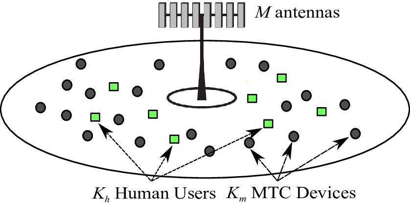
We consider the uplink of a single-cell mMIMO system where a BS with $M$ antennas is serving $K$ single-antenna devices. An example setup is illustrated in Fig. 1. There are two types of devices based on the communication they require. Among these devices $K_{m}$ of them, referred to as machines, require machine-type communication and the remaining $K_{h}=K-K_{m}$ devices, referred to as humans, generate human-type traffic. Humans are assumed to be smaller in numbers and require higher data rates compared to machines.

The time-frequency resources are divided into coherence intervals (CI), such that each channel is constant and frequency-flat in each interval [13]. In each CI, the channels take independent realizations from stationary ergodic processes. In the massive MIMO context, a CI consists of the following phases: uplink training, uplink data transmission. The downlink data transmission can either take place in the same CI (as in time-division duplex) or in other dedicated CIs (as in frequency-division duplex). In this paper, we focus on the uplink training and uplink data transmission, while the downlink data transmission analysis is left as future work. Each CI has length $N$ (in samples) and a fraction of these samples are reserved for training whereas the remaining ones are utilized for uplink data transmission. The allocation of samples varies among the schemes considered and the details are provided in Section II-A.

Non-line-of-sight communication is assumed and the channel between device $k$ and the BS is modeled as

$$\mathbf{g}_{k}=\sqrt{\beta_{k}}\mathbf{h}_{k},\forall k=1,\ldots,K,$$

(1)

where $\beta_{k}$ is the large-scale fading and $\mathbf{h}_{k}$ is the small-scale fading. Each element of $\mathbf{h}_{k}$ is modeled as i.i.d.$~\mathsf{CN}(0,1)$. The large-scale fading coefficients are assumed to be identical across antennas and known at the BS as they usually change very slowly which makes it possible to acquire accurate estimates. However, the small-scale fading coefficients change independently between CIs and are to be estimated in each CI via uplink training.

In conventional mMIMO setups, all $K$ devices concurrently transmit their pilot sequences and BS estimates the channels based on the received signal. The estimates acquired via this process, referred as uplink training, are utilized to design combining vectors for uplink data transmission (and precoding vectors for downlink data transmission).

The pilot sequences are generally assumed to be mutually orthogonal for users within a cell. These assumptions on pilot sequences are not realistic for some scenarios in future wireless networks, such as massive MTC with a large number of devices, since it requires many pilots and cumbersome access procedures for pilot assignment [6]. Moreover, constraints on the uplink power budget and excessive overhead signaling compel the use of non-orthogonal pilots for MTC [2, 16].

In this work, it is assumed that the humans require higher data rates and are smaller in numbers compared to machines, i.e., $K_{h}<K_{m}$. As a result, the humans have the privilege to orthogonal pilots, whereas it is not possible to assign orthogonal pilot to machines due to the large number of machines. Moreover, machines are assumed to be low-powered, and low complexity devices which require lower rates. Hence, allocating orthogonal resources to machines requires excessive overhead signaling¹¹ 1 There are exceptions to the low data rate assumption of machines, such as surveillance applications [17]. In these cases the machines with high data rate requirements may be treated as humans..

Let $\sqrt{N_{p}}\boldsymbol{\varphi}_{k}\in\mathbb{C}^{N_{p}\times 1}$ denote the $N_{p}$-length pilot signal for the $k$th device with $\|\boldsymbol{\varphi}_{k}\|^{2}=1$. It is assumed that humans are always allocated orthogonal pilots. Hence,

$$\boldsymbol{\varphi}_{k}^{H}\boldsymbol{\varphi}_{i}=0,~~~\forall k\in\{1,\ldots,K_{h}\},\forall i\in\{1,\ldots,K\}\setminus\{k\},$$

(2)

with SC-$2$ and

$$\boldsymbol{\varphi}_{k}^{H}\boldsymbol{\varphi}_{i}=0,~~~\forall k\in\{1,\ldots,K_{h}\},\forall i\in\{1,\ldots,K_{h}\}\setminus\{k\},$$

(3)

with SC-$1$ and SC-$3$.

For machines, non-orthogonal pilots are utilized and we investigate the problem of designing optimal non-orthogonal sequences in terms of channel estimation error. In SC-$1$ and SC-$2$, the active devices concurrently transmit their pilot sequences and the composite received signal at the BS is

$$\mathbf{Y}=\sqrt{N_{p}}\sum\limits_{k^{\prime}\in\mathcal{K}_{1}}\sqrt{q_{k^{\prime}}}\mathbf{g}_{k^{\prime}}\boldsymbol{\varphi}_{k^{\prime}}^{H}+\mathbf{Z},$$

(4)

in SC-$1$. Here, $\mathbf{Z}\in\mathbb{C}^{M\times N_{p}}$ is the noise matrix with i.i.d.$~\mathsf{CN}(0,\sigma^{2})$ elements and $q_{k^{\prime}}$ denotes the transmission power of pilot symbols for user $k^{\prime}$. The set of active devices $\mathcal{K}_{1}$ is either equal to $\mathcal{K}_{m}$ or $\mathcal{K}_{h}$, i.e., the set of machines or humans. In SC-$2$ the received signal at the BS is

$$\mathbf{Y}=\sqrt{N_{p}}\sum\limits_{k^{\prime}\in\mathcal{K}_{h}}\sqrt{q_{k^{\prime}}}\mathbf{g}_{k^{\prime}}\boldsymbol{\varphi}_{k^{\prime}}^{H}+\sqrt{N_{p}}\sum\limits_{k^{\prime}\in\mathcal{K}_{m}}\sqrt{q_{k^{\prime}}}\mathbf{g}_{k^{\prime}}\boldsymbol{\varphi}_{k^{\prime}}^{H}+\mathbf{Z},$$

(5)

In SC-$3$, the humans transmit data while machines are training and the composite received signal at the BS during the training of machines is

$$\mathbf{Y}=\sum\limits_{k^{\prime}\in\mathcal{K}_{h}}\hskip-5.69046pt\mathbf{g}_{k^{\prime}}\mathbf{x}_{k^{\prime}}^{H}+\sqrt{N_{p}^{m}}\hskip-5.69046pt\sum\limits_{k^{\prime}\in\mathcal{K}_{m}}\hskip-5.69046pt\sqrt{q_{k^{\prime}}}\mathbf{g}_{k^{\prime}}\boldsymbol{\varphi}_{k^{\prime}}^{H}+\mathbf{Z}$$

(6)

where $\mathbf{x_{k}}=\sqrt{p_{k}}\mathbf{s_{k}}$ and each element of $\mathbf{s_{k}}$ is a unit power symbol to be conveyed by device $k$. In this work, our focus is on the design of optimal non-orthogonal pilot sequences and we leave the joint pilot and data transmit power control problem as future work. Under this assumption, the first term in (6) can be treated as additive (but not Gaussian) noise. This allows us focus on the training of machines with non-orthogonal pilots and to generalize (4), (5), and (6) as

$$\mathbf{Y}=\sqrt{N_{p}}\sum\limits_{k^{\prime}\in\mathcal{K}}\sqrt{q_{k^{\prime}}}\mathbf{g}_{k^{\prime}}\boldsymbol{\varphi}_{k^{\prime}}^{H}+\tilde{\mathbf{Z}},$$

(7)

where the set of active devices depends on the scheme.

In order to estimate the channel of device $k\in\mathcal{K}_{m}$, the BS performs a de-spreading operation on the received signal:

	$\displaystyle\mathbf{y}_{k}$	$\displaystyle=$	$\displaystyle\mathbf{Y}\boldsymbol{\varphi}_{k},$		(8)
		$\displaystyle=$	$\displaystyle\sqrt{N_{p}q_{k}}\mathbf{g}_{k}+\sqrt{N_{p}}\hskip-5.69046pt\sum\limits_{k^{\prime}\in\mathcal{K}_{m}\backslash\{k\}}\hskip-5.69046pt\sqrt{q_{k}}\mathbf{g}_{k^{\prime}}\boldsymbol{\varphi}_{k^{\prime}}^{H}\boldsymbol{\varphi}_{k}+\mathbf{z}^{\prime},$
		$\displaystyle=$	$\displaystyle\hskip-5.69054pt\sqrt{N_{p}\beta_{k}q_{k}}\mathbf{h}_{k}\hskip-2.84526pt+\hskip-2.84526pt\sqrt{N_{p}}\hskip-11.38092pt\sum\limits_{k^{\prime}\in\mathcal{K}_{m}\backslash\{k\}}\hskip-11.38092pt\sqrt{\beta_{k^{\prime}}q_{k^{\prime}}}\mathbf{h}_{k^{\prime}}\boldsymbol{\varphi}_{k^{\prime}}^{H}\boldsymbol{\varphi}_{k}\hskip-2.84526pt+\mathbf{z}^{\prime},$

where $\mathbf{z}^{\prime}=\tilde{\mathbf{Z}}\boldsymbol{\varphi}_{k}$ has i.i.d.$~\mathsf{CN}(0,\sigma^{2})$ elements, since $\|\boldsymbol{\varphi}_{k}\|^{2}=1$, for SC-$1$ and SC-$2$. For SC-$3$, $\mathbf{z}^{\prime}$ has i.i.d. elements, however it is not necessarily Gaussian. Then, the BS either utilizes the least squares (LS) estimator or linear minimum mean-square error (LMMSE) estimator to obtain the channel estimate $\hat{\mathbf{h}}_{k}$. The LS estimate for device $k$ is,

	$\displaystyle\hat{\mathbf{h}}^{\textrm{LS}}_{k}$	$\displaystyle=$	$\displaystyle\mathbf{y}_{k}(\sqrt{N_{p}\beta_{k}q_{k}})^{-1},$		(9)
		$\displaystyle=$	$\displaystyle\mathbf{h}_{k}+\frac{\sum_{k^{\prime}\in\mathcal{K}_{m}\backslash\{k\}}\sqrt{N_{p}\beta_{k^{\prime}}q_{k^{\prime}}}\mathbf{h}_{k^{\prime}}\boldsymbol{\varphi}_{k^{\prime}}^{H}\boldsymbol{\varphi}_{k}+\mathbf{z}^{\prime}}{\sqrt{N_{p}\beta_{k}q_{k}}}.$

The estimation error for device $k$ is

	$\displaystyle\tilde{\mathbf{h}}_{k}^{\textrm{LS}}$	$\displaystyle=$	$\displaystyle\hat{\mathbf{h}}^{\textrm{LS}}_{k}-\mathbf{h}_{k},$		(10)
		$\displaystyle=$	$\displaystyle\frac{\sum_{k^{\prime}\in\mathcal{K}_{m}\backslash\{k\}}\sqrt{N_{p}\beta_{k^{\prime}}q_{k^{\prime}}}\mathbf{h}_{k^{\prime}}\boldsymbol{\varphi}_{k^{\prime}}^{H}\boldsymbol{\varphi}_{k}+\mathbf{z}^{\prime}}{\sqrt{N_{p}\beta_{k}q_{k}}}.$		(11)

The mean square of the $m$th element of $\tilde{\mathbf{h}}_{k}^{\textrm{LS}}$ with respect to the small-scale fading coefficients, $\mathbf{h}$ and noise, $\mathbf{z}$, is given by

	$\displaystyle e_{k}^{\textrm{LS}}$	$\displaystyle=$	$\displaystyle\mathbb{E}_{\mathbf{h},\mathbf{z}}\left[\left|\left[\tilde{\mathbf{h}}_{k}^{\textrm{LS}}\right]_{m}\right|^{2}\right]$		(12)
		$\displaystyle=$	$\displaystyle\frac{N_{p}\sum_{k^{\prime}\in\mathcal{K}_{m}\backslash\{k\}}\beta_{k^{\prime}}q_{k^{\prime}}\left|\boldsymbol{\varphi}_{k^{\prime}}^{H}\boldsymbol{\varphi}_{k}\right|^{2}+\sigma^{2}}{N_{p}\beta_{k}q_{k}}.$		(13)

Next, we consider the LMMSE estimator which is widely used in the massive MIMO context [13]. The channel estimate given by the LMMSE estimator based on (8) is as follows:

$$\hat{\mathbf{h}}_{k}^{\textrm{LMMSE}}=\frac{\sqrt{N_{p}\beta_{k}q_{k}}}{N_{p}\sum\limits_{k^{\prime}\in\mathcal{K}_{m}}\beta_{k^{\prime}}q_{k^{\prime}}|\boldsymbol{\varphi}_{k^{\prime}}^{H}\boldsymbol{\varphi}_{k}|^{2}+\sigma^{2}}\mathbf{y}_{k}.$$

(17)

The LMMSE estimate $\hat{\mathbf{h}}_{k}^{\textrm{LMMSE}}$ has $M$ i.i.d. elements and the mean-square of the $m$th component is

$\displaystyle\gamma_{k}=\mathbb{E}_{\mathbf{h},\mathbf{z}}\left[\left|\left[\hat{\mathbf{h}}_{k}^{\mathrm{LMMSE}}\right]_{m}\right|^{2}\right]=\frac{N_{p}\beta_{k}q_{k}}{N_{p}\sum\limits_{k^{\prime}\in\mathcal{K}_{m}}\beta_{k^{\prime}}q_{k^{\prime}}|\boldsymbol{\varphi}_{k^{\prime}}^{H}\boldsymbol{\varphi}_{k}|^{2}+\sigma^{2}},$

(18)

where $\mathbb{E}_{\mathbf{h},\mathbf{z}}$ denotes the expectation with respect to $m$th component of $\mathbf{h}$ and $\mathbf{z}$. Let $\tilde{\mathbf{h}}_{k}^{\mathrm{LMMSE}}=\hat{\mathbf{h}}_{k}^{\mathrm{LMMSE}}-\mathbf{h}_{k}$ denote the channel estimation error of device $k$ and the mean-square estimation error of the $m$th component is given by

$\displaystyle e_{k}^{\mathrm{LMMSE}}=\mathbb{E}_{\mathbf{h},\mathbf{z}}\left[\left|\left[\tilde{\mathbf{h}}_{k}^{\mathrm{LMMSE}}\right]_{m}\right|^{2}\right]=1-\frac{N_{p}\beta_{k}q_{k}}{N_{p}\sum\limits_{k^{\prime}\in\mathcal{K}_{m}}\beta_{k^{\prime}}q_{k^{\prime}}|\boldsymbol{\varphi}_{k^{\prime}}^{H}\boldsymbol{\varphi}_{k}|^{2}+\sigma^{2}}.$

(19)

For the cases where humans transmit data during machines training (SC-$3$), the LMMSE estimator is no longer the true MMSE estimator, however, the succeeding analysis is still valid for all the schemes considered.

We consider the problem of min-max estimation error optimization and aim to find the optimal pilot sequences for machines which provide the min-max solution

$$e^{*}=\min_{\mathbf{q},\boldsymbol{\phi}}\max_{k\in\mathcal{K}_{m}}~e_{k},$$

(20)

where the minimization is with respect to the pilot transmission powers, $\mathbf{q}=[q_{1},\ldots,q_{K_{m}}]^{T}$, and pilot sequences, $\boldsymbol{\phi}$. First, we investigate the case without any power constraints, i.e., each element of $\mathbf{q}$ is only assumed to be non-negative. The case with power constraints is analyzed in Section III-B. The set of pilot sequences considered, $\boldsymbol{\phi}$ contains vectors of the form $\sqrt{N_{p}}\boldsymbol{\varphi}_{k}$ with, where $\boldsymbol{\varphi}_{k}\in\mathbb{C}^{N_{p}\times 1}$ and $\|\boldsymbol{\varphi}_{k}\|^{2}=1$ for all $k\in\mathcal{K}_{m}$.

First note that, $e^{*}$ is achieved when $e_{1}=e_{2}=\ldots=e_{K}$ which can be proved as follows. Suppose $e^{*}$ can only be achieved when devices have different $e_{k}$’s and consider a case where $e_{1}<e_{2}=\ldots,=e_{K}=e^{*}$ for a given pilot sequence. Then, by reducing the transmit power, $q_{1}$, of device $1$, it is possible to obtain a smaller or equal error for other devices which results in $e^{*}=e_{1}=e_{2}=\ldots=e_{K}$. This contradicts the initial assumption that $e^{*}$ can only be achieved when devices have different channel estimation errors.

Consider the least-squares estimator error given by (12) which can be rewritten in vector notation as

$$\mathbf{\Phi}\boldsymbol{\mu}+\boldsymbol{\eta}=e\boldsymbol{\mu},$$

(21)

where

$$\mathbf{\Phi}=\begin{bmatrix}0&\left|\boldsymbol{\varphi}_{2}^{H}\boldsymbol{\varphi}_{1}\right|^{2}&\ldots&\left|\boldsymbol{\varphi}_{K}^{H}\boldsymbol{\varphi}_{1}\right|^{2}\\ \left|\boldsymbol{\varphi}_{1}^{H}\boldsymbol{\varphi}_{2}\right|^{2}&0&\ldots&\left|\boldsymbol{\varphi}_{K}^{H}\boldsymbol{\varphi}_{2}\right|^{2}\\ \vdots&&\ddots&\vdots\\ \left|\boldsymbol{\varphi}_{1}^{H}\boldsymbol{\varphi}_{K}\right|^{2}&\ldots&&0\end{bmatrix},$$

(22)

and

$$\boldsymbol{\mu}=[\mu_{1},\dots,\mu_{K}]^{T},$$

(23)

with $\mu_{j}=\beta_{j}q_{j}$ for all $j\in\mathcal{K}_{m}$. $e$ is the squared error aimed for each device and the normalized noise vector is

$$\boldsymbol{\eta}=\frac{\sigma^{2}}{N_{p}}\mathbf{1},$$

(24)

where $\mathbf{1}$ is the all ones vector. Re-writing (21) as

$$\frac{1}{1+e}\bar{\mathbf{\Phi}}\boldsymbol{\mu}+\bar{\boldsymbol{\eta}}=\boldsymbol{\mu},$$

(25)

where $\bar{\mathbf{\Phi}}=\mathbf{\Phi}+\mathbf{I}$ and $\bar{\boldsymbol{\eta}}=\boldsymbol{\eta}/(1+e)$, the minimum power solution for a given $e$ is

$$\boldsymbol{\mu}^{*}=\left(\mathbf{I}-\frac{1}{1+e}\bar{\mathbf{\Phi}}\right)^{-1}\bar{\boldsymbol{\eta}},$$

(26)

and there exist a positive $\boldsymbol{\mu}$ such that the mean square channel estimation error is $e$ for each device if and only if the spectral radius of $\bar{\mathbf{\Phi}}$, denoted by $\rho(\bar{\mathbf{\Phi}})$, is less than $1+e$ [18]. Note that, it is assumed that there are no constraint on pilot transmit powers to make the problem tractable (Similar result may be obtained by assuming the thermal noise is negligible) and the investigation under a setup with power constraints is presented in Section III-B. Based on (26), the following can be stated.

An important observation is that $e^{*}$ is independent of the pilot transmission powers and only depends on the expected correlation between the pilot sequences. Next, we investigate the minimum spectral radius of $\bar{\mathbf{\Phi}}$.

$\bar{\mathbf{\Phi}}$ is a non-negative matrix by definition and hence $\rho(\bar{\mathbf{\Phi}})$ is an eigenvalue of $\bar{\mathbf{\Phi}}$ [19, Theorem 8.3.1]. Furthermore, it is a symmetric matrix and a bound on its spectral radius is given by the following lemma.

Using the Jensen’s inequality, Lemma 2 can be extended as follows

$$\sqrt{\frac{\sum_{i=1}^{L}d_{i}^{2}}{L}}\geq\frac{1}{L}\sum_{i=1}^{L}d_{i}$$

(28)

with equality if and only if $d_{1}=d_{2}\ldots,=d_{n}$. Using the bounds given in (27) and (28) on $\bar{\mathbf{\Phi}}$, we obtain

$$\rho(\bar{\mathbf{\Phi}})\geq\sqrt{\frac{\sum_{i=1}^{K_{m}}\left(\sum_{j=1}^{K_{m}}|\boldsymbol{\varphi}_{i}^{H}\boldsymbol{\varphi}_{j}|^{2}\right)^{2}}{K_{m}}}\geq\frac{1}{K_{m}}\sum_{i=1}^{K_{m}}\sum_{j=1}^{K_{m}}|\boldsymbol{\varphi}_{i}^{H}\boldsymbol{\varphi}_{j}|^{2}\geq\frac{K_{m}}{N_{p}},$$

(29)

where the last inequality follows from the Welch bound [21], defined in Appendix A. Any set of vectors satisfying Welch bound is known as Welch bound equality sequences (WBE). Furthermore, any WBE sequence, $\boldsymbol{\varphi}_{1},\ldots,\boldsymbol{\varphi}_{K_{m}}$ in $\mathbb{C}^{N_{p}}$, has the following property [22]

$$\sum_{j=1}^{K_{m}}|\boldsymbol{\varphi}_{i}^{H}\boldsymbol{\varphi}_{j}|^{2}=\frac{K_{m}}{N_{p}},~~\forall i=1,\ldots,K_{m}.$$

(30)

Hence, WBE sequences satisfy the inequalities in (29) with equality and provides the minimum $\rho(\bar{\mathbf{\Phi}})=K_{m}/N_{p}$. Based on Lemma 1, it can be concluded that WBE sequences minimizes the min-max total squared channel estimation error for the LS estimator. Furthermore, a similar analysis based on (16) reveals that WBE sequences also minimize the min-max total squared channel estimation error for random pilot allocation schemes with the LS estimator.

Similarly, the mean square error for the LMMSE estimator given by (19) can be rewritten in vector notation as follows

$$\left(1-e\right)\left(\bar{\mathbf{\Phi}}\boldsymbol{\mu}+\boldsymbol{\eta}\right)=\boldsymbol{\mu},$$

(31)

and the minimum power solution is

$$\boldsymbol{\mu}^{*}=\left(\mathbf{I}-\left(1-e\right)\bar{\mathbf{\Phi}}\right)^{-1}\left(1-e\right)\boldsymbol{\eta}.$$

(32)

Similar to the LS case, there exist a positive $\boldsymbol{\mu}$ such that the mean square channel estimation error is $e$ for each device if and only if $\rho(\bar{\mathbf{\Phi}})$, is less than $1/\left(1-e\right)$ [18]. The rest of the analysis follows the same steps given in LS case and is therefore omitted. A crucial difference with the MMSE estimator case is that only deterministic pilot allocation schemes are considered, i.e., $\mathbb{E}\left[|\boldsymbol{\varphi}_{i}^{H}\boldsymbol{\varphi}_{j}|^{2}\right]=|\boldsymbol{\varphi}_{i}^{H}\boldsymbol{\varphi}_{j}|^{2}$. Hence, the performance of random allocation schemes with MMSE estimator are investigated numerically.

The analysis provided above allows us to state the following result regarding the optimal pilot sequences.

Theorem 1 considers pilot sequences with length $N_{p}\leq K_{m}$ and when $K_{m}=N_{p}$ the pilot sequences becomes orthogonal. The definition of Welch bound and sequences satisfying the bound is given in Appendix A.

The design of WBE codes is fairly straightforward and extensively investigated in the literature [23]. An example of a structured WBE codebook is given in [24], which utilizes normalized $N_{p}$ distinct rows of a $K_{m}\times K_{m}$ FFT matrix. The pilot sequence for device $k$ is

$$\boldsymbol{\varphi}_{k}=\frac{1}{\sqrt{N_{p}}}\begin{bmatrix}e^{j\frac{2\pi}{K_{m}}u_{1}\left(k-1\right)}\\ e^{j\frac{2\pi}{K_{m}}u_{2}\left(k-1\right)}\\ \vdots\\ e^{j\frac{2\pi}{K_{m}}u_{N_{p}}\left(k-1\right)}\end{bmatrix}$$

(33)

where $\mathbf{u}=\left[u_{1},\ldots,u_{N_{p}}\right]^{T}$ is a vector consisting of $N_{p}$ parameters is to be selected. A simple choice of $u_{i}=i$ for all $i=1,\ldots,N_{p}$ provides a set of WBE sequences without any consideration of min-max correlation. Hence, assuming that the set of active devices is known, each device can generate its pilot sequence using (33).

In this section, the achievable rates of the three schemes illustrated in Fig. 2 are investigated. Each scheme has an uplink training phase followed by data transmission. Although we consider the case where the channel estimates are acquired via LMMSE estimator, the extension to LS estimators or other alternative estimators is straight-forward.

References

- [1] K. Senel, E. Björnson, and E. G. Larsson, “Humans and machine type communications can coexist in uplink massive MIMO systems,” in IEEE International Conference on Acoustics, Speech and Signal Processing (ICASSP), 2018.
- [2] Z. Dawy, W. Saad, A. Ghosh, J. G. Andrews, and E. Yaacoub, “Toward massive machine type cellular communications,” IEEE Wireless Communications, vol. 24, no. 1, pp. 120–128, 2017.
- [3] 3rd Generation Partnership Project (3GPP), “Cellular system support for ultra low complexity and low throughput internet of things,” Technical Specification Group GSM/EDGE Radio Access Network, Release 13, June 2015.
- [4] P. Popovski et al., “Final report on the METIS 5G system concept and technology roadmap,” METIS Document ICT-317669-METIS/D6.6, 2015.
- [5] A. Osseiran, F. Boccardi, V. Braun, K. Kusume, P. Marsch, M. Maternia, O. Queseth, M. Schellmann, H. Schotten, H. Taoka et al., “Scenarios for 5G mobile and wireless communications: the vision of the METIS project,” IEEE Communications Magazine, vol. 52, no. 5, pp. 26–35, 2014.
- [6] E. De Carvalho, E. Björnson, J. H. Sørensen, E. G. Larsson, and P. Popovski, “Random Pilot and Data Access in Massive MIMO for Machine-Type Communications,” IEEE Transactions on Wireless Communications, vol. 16, no. 12, pp. 7703–7717, 2017.
- [7] H. Wang, W. Zhang, Y. Liu, Q. Xu, and P. Pan, “On design of non-orthogonal pilot signals for a multi-cell massive MIMO system,” IEEE Wireless Communications Letters, vol. 4, no. 2, pp. 129–132, 2015.
- [8] N. Akbar, N. Yang, P. Sadeghi, and R. A. Kennedy, “Multi-cell multiuser massive MIMO networks: User capacity analysis and pilot design,” IEEE Transactions on Communications, vol. 64, no. 12, pp. 5064–5077, 2016.
- [9] C. S. Bontu, S. Periyalwar, and M. Pecen, “Wireless wide-area networks for internet of things: An air interface protocol for IoT and a simultaneous access channel for uplink IoT communication,” IEEE Vehicular Technology Magazine, vol. 9, no. 1, pp. 54–63, 2014.
- [10] G. J. Sutton, R. P. Liu, and Y. J. Guo, “Harmonising coexistence of Machine Type Communications with Wi-Fi data traffic under frame-based LBT,” IEEE Transactions on Communications, vol. 65, no. 9, pp. 4000–4011, 2017.
- [11] M. Centenaro, L. Vangelista, A. Zanella, and M. Zorzi, “Long-range communications in unlicensed bands: The rising stars in the IoT and smart city scenarios,” IEEE Wireless Communications, vol. 23, no. 5, pp. 60–67, 2016.
- [12] A. Biral, M. Centenaro, A. Zanella, L. Vangelista, and M. Zorzi, “The challenges of M2M massive access in wireless cellular networks,” Digital Communications and Networks, vol. 1, no. 1, pp. 1–19, 2015.
- [13] T. L. Marzetta, E. G. Larsson, H. Yang, and H. Q. Ngo, Fundamentals of Massive MIMO. Cambridge University Press, 2016.
- [14] Z. Jiang, B. Han, P. Chen, F. Yang, and Q. Bi, “On novel access and scheduling schemes for IoT communications,” Mobile Information Systems, vol. 2016, 2016.
- [15] L. Liu, E. G. Larsson, W. Yu, P. Popovski, C. Stefanovic, and E. De Carvalho, “Sparse signal processing for grant-free massive IoT connectivity,” IEEE Signal Processing Magazine, 2018, to appear.
- [16] E. De Carvalho, E. Björnson, J. H. Sorensen, P. Popovski, and E. G. Larsson, “Random access protocols for massive MIMO,” IEEE Communications Magazine, vol. 55, no. 5, pp. 216–222, 2017.
- [17] R. Ratasuk, J. Tan, and A. Ghosh, “Coverage and capacity analysis for machine type communications in LTE,” in Vehicular Technology Conference (VTC Spring), 2012 IEEE 75th. IEEE, 2012, pp. 1–5.
- [18] S. U. Pillai, T. Suel, and S. Cha, “The Perron-Frobenius theorem: some of its applications,” IEEE Signal Processing Magazine, vol. 22, no. 2, pp. 62–75, 2005.
- [19] R. A. Horn and C. R. Johnson, Matrix analysis. Cambridge University Press, 1990.
- [20] Z. Bo, “On the spectral radius of nonnegative matrices,” Australasian Journal of Combinatorics, vol. 22, pp. 301–306, 2000.
- [21] L. Welch, “Lower bounds on the maximum cross correlation of signals (Corresp.),” IEEE Transactions on Information theory, vol. 20, no. 3, pp. 397–399, 1974.
- [22] S. Waldron, “Generalized Welch bound equality sequences are tight frames,” IEEE Transactions on Information Theory, vol. 49, no. 9, pp. 2307–2309, 2003.
- [23] P. Xia, S. Zhou, and G. B. Giannakis, “Achieving the Welch bound with difference sets,” IEEE Transactions on Information Theory, vol. 51, no. 5, pp. 1900–1907, 2005.
- [24] B. M. Hochwald, T. L. Marzetta, T. J. Richardson, W. Sweldens, and R. Urbanke, “Systematic design of unitary space-time constellations,” IEEE transactions on Information Theory, vol. 46, no. 6, pp. 1962–1973, 2000.
- [25] E. Björnson, J. Hoydis, and L. Sanguinetti, “Massive MIMO networks: Spectral, energy, and hardware efficiency,” Foundations and Trends® in Signal Processing, vol. 11, no. 3-4, pp. 154–655, 2017. [Online]. Available: http://dx.doi.org/10.1561/2000000093
- [26] M. Medard, “The effect upon channel capacity in wireless communications of perfect and imperfect knowledge of the channel,” IEEE Transactions on Information theory, vol. 46, no. 3, pp. 933–946, 2000.
- [27] M. Grant and S. Boyd, “CVX: Matlab software for disciplined convex programming, version 2.1,” http://cvxr.com/cvx, Mar. 2014.
- [28] E. Björnson, E. G. Larsson, and M. Debbah, “Massive MIMO for maximal spectral efficiency: How many users and pilots should be allocated?” IEEE Transactions on Wireless Communications, vol. 15, no. 2, pp. 1293–1308, 2016.