Closed-Form Word Error Rate Analysis for Successive Interference Cancellation DecodersThanks: This work was presented in part at the 2017 IEEE International Conference on Communications (ICC), Paris, France.Thanks: J. Wen is with the College of Information Science and Technology, and the College of Cyber Security, Jinan University, Guangzhou 510632, China (e-mail: jinming.wen@mail.mcgill.ca).Thanks: K. Wu is with the School of Electronic Science, National University of Defense Technology, Changsha 410073, China (e-mail: keyuwu@nudt.edu.cn).Thanks: C. Tellambura is with the Department of Electrical and Computer Engineering, University of Alberta, Edmonton T6G 2V4, Canada (e-mail: chintha@ece.ualberta.ca)Thanks: P. Fan is with the Institute of Mobile Communications, Southwest Jiaotong University, Chengdu 610031, China (e-mail: p.fan@ieee.org)Thanks: The work of Pingzhi Fan was supported by NSFC-NRF project under grant No.61661146003/NRF2016NRF-NSFC001-089, and the 111 Project under Grant 111-2-14. This work was also partially supported by National Natural Science Foundation of China (No. 11871248), “the Fundamental Research Funds for the Central Universities” (No. 21618329) and the postdoc research fellowship from Fonds de Recherche Nature et Technologies.
Abstract
We consider the estimation of an integer vector from the linear observation , where is a random matrix with independent and identically distributed (i.i.d.) standard Gaussian entries, and is a noise vector with i.i.d. entries with given . In digital communications, is typically uniformly distributed over an -dimensional box . For this estimation problem, successive interference cancellation (SIC) decoders are popular due to their low complexity, and a detailed analysis of their word error rates (WERs) is highly useful. In this paper, we derive closed-form WER expressions for two cases: (1) is fixed and (2) is uniformly distributed over . We also investigate some of their properties in detail and show that they agree closely with simulated word error probabilities.
Index Terms:
Word error rate, successive interference cancellation, Babai’s nearest plane algorithm, integer least-squares problems.I Introduction
I-A Motivation
Integer parameter estimation [1] in linear models finds many applications such as Global Positioning System (GPS), cryptography, digital communications, code division multiple access and others. The prototype problem is to estimate (detect) an integer vector from the linear model:
| (1) |
where is an observation vector, is a random matrix with i.i.d. standard Gaussian entries and is a Gaussian noise vector with variance of each entry.
The maximum-likelihood (ML) estimator of is the solution of a simple least-squares problem if the integer constraint is relaxed (e.g., ). However, such relaxation is not highly accurate. Thus, the exact ML estimator of is given by the solution of the following integer least-squares (ILS) problem [1] [2]:
| (2) |
Because solving (2) is equivalent to finding the closest point to in the lattice , problem (2) is also referred to as the closest-point problem in cryptography [3]. In terms of complexity, this problem is Non-deterministic Polynomial (NP)-hard.
In digital communication links, prior to transmission, data bits are mapped to a fixed set of modulation symbols (signal constellation). For example, Section IV discusses -ary pulse amplitude modulation (PAM) constellation, which consists of integers. Thus, with -ary PAM, the entries of are selected from the fixed constellation of integers. The signal constellations are also subject to the average power constraints. Thus, the parameter vector satisfies a box constraint [4, 5, 6, 7, 8], i.e.,
| (3) |
In practical systems, all signal constellation points are equally likely, which is equivalent to being uniformly distributed over , see, e.g., [9, 10]. Thus, the box constraint (3) can be incorporated in (2), which yields the so-called box-constrained integer least-squares (BILS) problem:
| (4) |
Problems (2) and (4) can be optimally solved by a sphere decoder (see [2] and [6]), which consists of pre-processing and search stages. For example, one can pre-process matrix by using the Lenstra-Lenstra-Lovász (LLL) algorithm [11], which reduces to a nearly orthogonal lattice basis, which improves the efficiency of the search stage. Other pre-processing strategies include Vertical-Bell Labs layered Space Time algorithm (V-BLAST) [12], Sorted QR Decomposition (SQRD) [13] and their variants [5, 6, 7]. Perhaps, the most frequently utilized discrete search algorithms for (2) or (4) are the Schnorr-Euchner search algorithm [14] and its variants [3, 4, 15, 16, 17, 18, 19].
It has respectively been shown in [20] and [9] that (2) and (4) are NP-hard problems; hence, for many applications, suboptimal algorithms are common. A popular one for solving (2) is the ordinary successive interference cancellation (OSIC) decoder, which is actually Babai’s nearest plane algorithm [21]. It can also be adapted to form a box-constrained SIC (BSIC) decoder, a suboptimal algorithm for (4). Interestingly, since the Schnorr-Euchner algorithm is a depth-first search, the first valid solution found by it, is in fact the OSIC decoder solution, also called Babai point [3, 22]. Similarly, the initial solution of the Schnorr-Euchner decoder of (4) is the BSIC decoder solution, which is a box-constrained Babai point [3, 4, 6, 10].
Analyzing the performance of decoders helps to design and characterize wireless communication links [23, 24, 25, 26, 27, 28, 29]. The most common decoder performance measures involve the error probability of the decoding process. Specifically, we utilize the error probability that the output of the decoder is not equal to the true integer vector , which is called word error rate (WER). The probability of correct detection is called the success probability [1, 22, 30, 10].
The WER characterization of both OSIC and BSIC decoders is useful [22, 10]. Indeed, with OSIC decoder solving (2) or a BSIC decoder solving (4), their WERs, respectively denoted by, and , serve as critical quality parameters. For instance, a suitable threshold can be setup a priori – if the WER is below is threshold – to indicate that the decoder can be used with confidence. In this case, the additional effort of optimally solving the ILS (2) or the BILS (4) yields diminishing returns. However, if or is above the threshold, then more accurate decoders, such as a sphere decoder (ML estimator), should be used. Even if one intends to solve the ILS (2) or the BILS (4) for ML estimator of , it is still of vital importance to compute or since they are often used to approximate their WER.
I-B Contributions
Closed-form expressions for and have respectively been given in [22] and [10] when in (1) is deterministic. Moreover, closed-form WER expressions for zero-forcing and BSIC decoders have been derived for when is a fixed integer vector and for when is uniformly distributed over for deterministic [31]. The relationship between WERs of zero-forcing and BSIC decoders was also investigated in [31]. However, all of these formulas are for deterministic . To the best of our knowledge, for random , the WER analysis for SIC decoders has been lacking. This paper fills this gap and derives closed-form WER expressions for both OSIC and BSIC cases. Specifically, the contributions can be summarized as follows:
- •
We derive a closed-form WER expression for the SIC decoder when is a fixed integer vector, and investigate some of the properties of . In particular, we rigorously show that tends to 0 when , which is the noise variance, tends to 0, and quantify the gap of for two sizes and (Section III)11 1 This paper was presented in part at 2017 IEEE International Conference on Communications (ICC) [32]..
- •
We derive a closed-form WER expression for BSIC decoder when is uniformly distributed over , and investigate some of its properties. In particular, we rigorously show that tends to 0 when tends to 0, and quantify the gap of for two sizes and (Section IV).
- •
We study the relationship between and . More precisely, we show that and they converge to one value as noise variance tends to 0 (Section V).
I-C Comparison with existing work
Many works have theoretically analyzed the performance of some commonly used decoders [23, 24, 25]. Although our closed-form WER analysis has some connections with those in [23, 24, 25], there are main differences between them. More specifically:
- 1.
Our closed-form expressions (see eq. (12) and eq. (28) in Sec. III and IV) for the WER of OSIC and BSIC decoders are simpler and more concise than [23, Theorem 1] (note that [23, eq. (14)] is more complicated than eq. (10)), [24, eq. (18)] and [25, Theorem 1]. Because of this simplicity, we can theoretically characterize the gap of the WER corresponding to two different dimensions of (Theorems 3 and 7). However, we do not find similar results in [23, 24, 25].
- 2.
Another common difference between this paper and [23, 24, 25] is the techniques for the WER analysis. Our main techniques for the WER analysis are the distribution of the triangular factor of the QR factorization of the random matrix , chain rule, random available transformation and the computational formulas of OSIC and BSIC which are simple and clear. The main techniques of the joint error probability analysis in [23] are the distribution of the triangular factor of the QR factorization of the random matrix , chain rule and a result from [33]. Reference [24] mainly uses the total probability theorem and some approximation techniques. The main technique of [25] is based on some analysis on n-PSK modulation. There are also some other differences between them, outlined below:
- 3.
Another difference between this paper and [23] is that our WER analysis is valid for any box , while [23] assumes that is a cube with the edge length , where is a positive integer. Since in some applications, such as when the constellations are 4-QAM, the edge length of does not satisfy for a positive integer , and the analysis of WER over an arbitrary box is still needed.
- 4.
Different from our paper which analyzes the WER of OSIC and BSIC decoders, [24] investigates the bit error rates of both minimum mean square error (MMSE)-non-SIC and MMSE-SIC. From eq.(7)-eq.(8) and [24, eq.s (2-7)], we can see that these two papers study the error performance of different decoders.
- 5.
There are three additional differences between this paper and [25]: firstly, our analysis is valid for any box , which is different from [25] that assumes is transformed from -PSK modulators. Secondly, the WER in this paper refers to the probability that a decoder does not successfully detect , which is different from the symbol error probability in [25] (please see [25, eq.s (18) and (22)]). Thirdly, we give closed-form expressions for the exact WER of OSIC and BSIC decoders, whereas [25] proposes an approximation of the symbol error probability of multiple-input and multiple-output-MMSE-SIC decoders.
The rest of the paper is organized as follows. In Section II, we introduce the computational details of OSIC and BSIC decoders. In Section III, we develop a closed-form expression for and investigate its properties. In Section IV, we develop closed-form and study its properties. The relationship between and is analyzed in Section V. Numerical simulations to verify the derived formulas are presented in Section VI. Finally, we summarize and discuss our results in Section VII.
Notation: For a vector , denotes its nearest integer vector, i.e., each entry of is rounded to its nearest integer (if there is a tie, rounding is downward), and denotes the -th element of . Let be the element of matrix at row and column . Let and respectively denote the WER of the SIC and BSIC decoders
II OSIC and BSIC decoders
In this section, we briefly introduce the computational details of OSIC and BSIC decoders.
III WER for OSIC Decoders
In this section, we derive closed-form and investigate its properties.
III-A WER for OSIC Decoders
This subsection derives the expression. To this end, we introduce two lemmas which are needed for the one dimensional case and for characterizing the distribution of the entries of in (5). We begin by introducing the first lemma.
Lemma 1.
Consider the following scalar linear model:
| (9) |
where is a fixed unknown parameter number, is a Gaussian noise term, and , which is independent with , is a chi-square random variable with degrees of freedom. Let , then
| (10) |
where
| (11) |
Proof.
See Appendix A. ∎
To derive the main theorem for , we introduce the following lemma from [35, P. 99].
Lemma 2.
Let the entries of be i.i.d. Gaussian terms. Then all , are independent. Moreover, and for .
To prove Theorem 1, we first use the chain rule of conditional probabilities to transform to the product of terms with each of them representing a one-dimensional conditional success probability. We use Lemma 1 to compute each term and finally obtain (12). The detail is in the proof below.
Proof.
Let
then by the chain rule of conditional probabilities, we have
Thus, to show (12), we show
| (13) | ||||
| (14) |
for .
Remark 1.
III-B Properties of OSIC Decoders
We now investigate some properties of . We begin with presenting the following important lemma, which can be used to show that tends to 0 if noise level tends to 0 for the one dimensional case.
Lemma 3.
For any integer , it holds that
| (20) |
By (21), we have the following result.
Theorem 2.
The WER (see (12)) of OSIC decoders is an increasing function of and . Moreover, it satisfies
| (22) |
Proof.
In many applications, matrix is a square matrix. For ease of notation, let the WER of OSIC decoder be when matrix is . The following results can be directly obtained from (12).
Theorem 3.
Let be two integers, then and , which are respectively the WER of OSIC decoders for sizes and satisfy
| (24) |
Theorem 3 quantifies the gap between two for two different sizes. Specifically, if noise level converges to 0, then by (21), is close to 1 for any integer . Thus, eq. (24) indicates that when noise level converges to 0, the difference between and is small, implying that the gap between and is very small as long as noise level is near 0. For more details, see the numerical experiments in Section VI.
IV WER for BSIC Decoders
As mentioned before, for digital wireless communications and other applications, is uniformly distributed over . For this condition, we analyze the WER of BSIC decoder.
IV-A WER for BSIC Decoders
To derive closed-form , we first introduce the following useful lemma, which analyzes the WER for one dimensional case.
Lemma 4.
Suppose that we have the scale linear model (9), where is uniformly distributed on , is a noise number following the Gaussian distribution , and , which is independent with , follows central chi-square distribution with degree of freedom. Let
| (25) |
Then satisfies
| (26) |
where for ,
| (27) |
with being defined in (11).
Proof.
See Appendix B. ∎
Theorem 4.
Since is uniformly distributed over , is uniformly distributed on for . Theorem 4 can be proved by using more or less the same techniques as that for Theorem 1, thus we omit its proof.
Remark 4.
IV-B WER Properties of BSIC Decoders
In this subsection, we study some properties of the WER expression. We first investigate the property of . Specifically, we have the following result.
Lemma 5.
For any fixed and , (see (27)) is a strictly decreasing function of , i.e., the following inequality holds for any :
| (30) |
Proof.
Theorem 5.
Let and be any two dimensional boxes that satisfy for , then the WER of BSIC decoders corresponding to and satisfy
| (31) |
Similar to the ordinary case, the following result holds.
Theorem 6.
The WER of BSIC decoders is an increasing function of and . Moreover it satisfies
Proof.
Similar to the proof of Theorem 2, one can see that is an increasing function of and .
Similar to OSIC decoders, for easy notation, we denote the WER of BSIC decoders for square matrix and a cube whose edge length is as . The following results can then be directly obtained from (28).
Theorem 7.
Let be two integers, then and satisfy
| (33) |
Similar to the case of OSIC, Theorem 7 quantifies the gap between two . Specifically, by (32), if is close to 0, then is close to 1 for any integer and . Thus, eq. (33) indicates that when is close to 0, the difference between and is very small, implying that the gap between and is very small as long as noise level is close to 0. For more details, see the numerical experiments in Section VI.
V Relationship between and
In this section, we investigate the relationship between and .We first investigate the relationship between and (see (10) and (27)). Specifically, we have the following result.
Theorem 8.
For any fixed and , if , then and satisfy
| (34) |
Moreover,
| (35) |
Proof.
By (12), (28) and Theorem 8, we obtain Theorem 9, which characterizes the relationship between and .
Theorem 9.
For any , and have the following relationship
| (36) |
Moreover,
Note that Theorem 9 also holds for deterministic , for more details, see [10, Corollary 1]. The inequality (36) shows that BSIC outperforms OSIC given the same level of noise. Intuitively this is because, in OSIC, can be anywhere in . In BSIC, is limited to finite number of choices, and this property seems to improve the detection accuracy. Theoretically, it can be showed by using (12), (28) and Theorem 8.
VI Numerical Experiments
We now provide simulations and numerical results to verify the accuracy of the WER formulas (12) and (28), which are compared against the simulated WER. Each simulation run is averaged over samples. For simplicity, we assume that in all of the following tests (our extensive simulations found that both (12) and (28) are accurate for both SIC and BSIC decoders for both and ).
We did the simulations by choosing a range of , and boxes (more details on the choice of these parameters are given subsequently). For each fixed and , we randomly generated ’s, whose entries independent and identically follow the standard Gaussian distribution , and ’s with each of them following the Gaussian distribution . To illustrate the effectiveness of (12), for each generated and , we randomly generated an . To verify the accuracy of (28), for each generated and , we randomly generated an which is uniformly distributed over a given . Then, we got linear models which satisfy (1) only, and another linear models which satisfy both (1) and (3). Then, we found and corresponding to each ordinary and box-constrained linear model according to (7) and (8), respectively. Finally, the number of events divided by was computed as the simulated WER for OSIC decoders. Similarly, the number of events divided by was computed as the simulated WER for BSIC decoders. The theoretical WERs are computed from (12) and (28) for SIC and BSIC decoders.
VI-A Numerical experiments for OSIC decoders
We investigate the OSIC WER to verify the accuracy of (12). Figure 1 shows the WER for several noise standard deviations and for several sizes . The results for are added to show the WER of OSIC decoder for large size. The theoretical and simulated WERs match very well, confirming the accuracy of (12). Theorem 2 states that increases when or increases. Indeed, Figure 1 clearly demonstrates the increasing trend of with noise level . As size increases, increases slightly and then plateaus. Although when noise variance is small, e.g., high-SNR region, is more or less constant irrespective of size .


We may use Theorem 3 to explain the above phenomena. The numerical values are depicted in Figure 2 for noise variance of and . For both cases, converges to 1 as increases. Therefore, for given , the performance difference between two OSIC detectors respectively with dimensions and () is negligible, if is sufficient large. Intuitively, this phenomenon is because, for OSIC, detection error is more likely to occur in early stages (see (13) and (14), and also notice that increases with ). Therefore, given that all previous stages are correctly detected, the probabilities of correct detection of later stages approach 1 (notice that approaches 1 for sufficient large ). Therefore, if is above a certain threshold, further increasing causes negligible performance deterioration.
VI-B WER performance of BSIC decoders
Here, we test the accuracy of (28). Since in wireless applications the box is generally a hypercube where and are fixed and the same for . Thus, we choose , , and for testing.


For a BSIC with (when for some integer ), each entry of can be viewed as a -ary pulse-amplitude modulation (PAM) baseband signal22 2 Strictly speaking, we have is equivalent to a -ary baseband signal, since communication signal is generally symmetric to the origin. . Furthermore, we evaluate BSIC WER in terms of signal-to-noise ratio (SNR), which is commonly used in wireless communications. For a BSIC with , the relationship (see Appendix C for proof) between and SNR in decibels (dB) is
Figures 3-4 show theoretical and simulated WER of BSIC decoders. SNR ranges from 10 to 30 dB. Each entry of are randomly selected from 2-PAM and 4-PAM, respectively. Figures 3-4 show that theoretical and simulated WERs match well which confirms the accuracy of (28). It can also be observed that when the size increases, the WER increases, which matches Theorem 6. Similar to the case of OSIC, due to the decreasing error propagation nature of BSIC, the performance deterioration caused by increasing vanishes as exceeds certain threshold (depending on SNR).
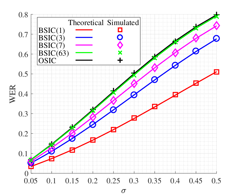
Figure 5 investigates WER of BSIC decoders with , , and , denoted by BSIC(1), BSIC(3), BSIC(7) and BSIC(63), respectively. For comparison, the OSIC with is also included (denoted as OSIC). It can be recognized that, for BSIC decoders, increasing the size increases WER. This observation matches with Theorem 5. Furthermore, the WER of OSIC decoder exceeds that of BSIC with the same and . Finally, when , appears to converge to . Theorem 9 predicts these trends.

To explain the above phenomena, we display under two noise levels and edge length in Figure 6. From Figure 6, one can see that converges to 1 rapidly, especially when . Also reminding that, in (33), we have
Therefore, we can conclude that should change slowly for sufficiently large , which explains the ’s trends along in Figures 3-4. In addition, one can observe that, for given and , gets smaller when becomes larger, which is confirmed via Lemma 5. This suggests that decoding performance under larger edge length decreases more with increasing . Finally, by comparing Figure 2 with Figure 6, it can be seen that is very close to , which is supported via Theorem 8. And this explains why with approaches in Figure 5.
VII Summary and discussions
In this paper, we have derived closed-form WER expressions and for OSIC and BSIC decoders, investigated certain properties of the expressions and studied their connections. The accuracy of these expressions has been verified via simulation and numerical results.
In our model, the entries of are i.i.d. standard Gaussian variables. The noise vector follows Gaussian distribution . This model can be readily extended to the complex case, which is important in practical applications. Thus, if the entries of and are i.i.d. complex Gaussian, and is also assumed to be a complex vector with both of its real and image parts being uniformly distributed over a box . Then just like the real case (see (5)), QR factorization of yields , are independent, and and for . One can easily obtain formulas for and under complex , and by using the techniques developed in this paper. Thus, we omit the details.
Theoretical results [22] show that the LLL reduction can always decrease (not strictly) for deterministic . It is straightforward to see that the LLL reduction can also always decrease (not strictly) for random . Thus, it is important to develop a formula for after the LLL reduction is performed on . But to do this, we need to find the distribution of the entries of , which is the LLL reduced matrix of (see (5)). However, to the best of our knowledge, this is still an open problem due to the complication of the LLL reduction.
It is well-known that some of the permutation strategies, such as V-BLAST [12] and SQRD [13], can usually decrease for deterministic . This property also holds for random . Thus, closed-form when is column permuted may be useful, which is a potential future research problem. In addition to these traditional detection strategies, one can also use a naive lattice decoder [37] to detect (e.g. perform traditional lattice decoding and discard the vectors not in the box [37]). The naive lattice decoder performs better for (4) than for the ordinary linear model. Furthermore, naive lattice decoding achieves maximum diversity [38]. Since this decoding is complicated, closed-form analysis of its WER appears intractable.
On the other hand, although the LLL reduction algorithm reduces -dimensional lattices, whose basis vectors are integer vectors, in polynomial time of (see [11], [39]), and the average complexity of reducing an i.i.d. Gaussian matrix is also a polynomial of the column rank of ([40], [41]), the worst-case complexity of LLL is not even finite [41]. This suggests a potential use for closed-form . For instance, if is smaller than a suitable threshold, we may not employ LLL reduction; thus, in practical applications, LLL reduction may be applied adaptively. Similarly, closed-form can be useful.
Minimum mean square error (MMSE) decoder is a popular alternative to OSIC and BSIC decoders. MMSE decoder adapts to the noise level [42]. A closed-form WER of MMSE is a potential future research topic.
Appendix A Proof of Lemma 1
Proof.
Let , and . Thus, if and only if . Thus, to show (10), we derive . Note that is the ratio of two independent central chi-square random variables. The distribution of this ratio is well-known [43, Section 27]. That is, where an distributed rv. Thus, the PDF of is given by
Therefore, we find
| (37) |
where the last equality follows from the substitution . Thus, the lemma holds. ∎
Appendix B Proof of Lemma 4
Proof.
Since is uniformly distributed on , we have
| (38) |
In the following, we derive formulas for
We first show how to compute . Since and are independent, by the distribution of and , we can see that the PDF of is symmetric with . Thus,
| (39) |
where is because , (b) follows from (37) and (c) is from (20).
Similarly, we have
| (40) |
Since the PDF of is symmetric with , we have
| (41) |
Appendix C Derivation of SNR
In the following, we give the relationship between SNR in dB and for the case that is uniformly distributed in a box ( for some integer ), which is transformed from an -dimensional -ary PAM. Specifically, for any signal in an -dimensional -ary PAM, i.e., , we let , where is an -dimensional vector with all of its entries being 1, then .
Since is transformed from an -dimensional -ary PAM, we calculate over the -dimensional -ary PAM instead of over . Since each entry of belongs to a -ary PAM, there are number of different , and hence
| (42) |
Each has entries, so the total number of entries of all the different are . Since is uniformly distributed over -dimensional -ary PAM, each entry of is also uniformly distributed over -ary PAM, which implies that each point in the -ary PAM are chosen
times. Therefore,
Then by (42), we have
Therefore, we SNR in dB satisfies
References
- [1] A. Hassibi and S. Boyd, “Integer parameter estimation in linear models with applications to GPS,” IEEE Trans. Signal Process., vol. 46, no. 11, pp. 2938–2952, Nov. 1998.
- [2] B. Hassibi and H. Vikalo, “On the sphere-decoding algorithm I. Expected complexity,” IEEE Trans. Signal Process., vol. 53, no. 8, pp. 2806–2818, Aug. 2005.
- [3] E. Agrell, T. Eriksson, A. Vardy, and K. Zeger, “Closest point search in lattices,” IEEE Trans. Inf. Theory, vol. 48, no. 8, pp. 2201–2214, Aug. 2002.
- [4] M. O. Damen, H. E. Gamal, and G. Caire, “On maximum likelihood detection and the search for the closest lattice point,” IEEE Trans. Inf. Theory, vol. 49, no. 10, pp. 2389–2402, Oct. 2003.
- [5] K. Su and I. J. Wassell, “A new ordering for efficient sphere decoding,” in Proc. IEEE Int. Conf. Commun. (ICC), May 2005, pp. 1906–1910.
- [6] X.-W. Chang and Q. Han, “Solving box-constrained integer least squares problems,” IEEE Trans. Wireless Commun., vol. 7, no. 1, pp. 277–287, Jan. 2008.
- [7] S. Breen and X. Chang, “Column reording for box-constrained integer least squares problems,” in Proc. IEEE Global Commun. Conf. (Globecom), Dec. 2011, pp. 1–6.
- [8] J. Park, J. Kim, and D. J. Love, “Antenna reliability ordering technique for unequal error protection in jointly detected MIMO systems,” IEEE Trans. Veh. Technol., vol. 65, no. 9, pp. 7136–7148, Sept. 2016.
- [9] J. Jaldén and B. Ottersten, “On the complexity of sphere decoding in digital communications,” IEEE Trans. Signal Process., vol. 53, no. 4, pp. 1474–1484, April 2005.
- [10] J. Wen and X.-W. Chang, “The success probability of the Babai point estimator and the integer least squares estimator in box-constrained integer linear models,” IEEE Trans. Inf. Theory, vol. 63, no. 1, pp. 631–648, Jan. 2017.
- [11] A. Lenstra, H. Lenstra, and L. Lovász, “Factoring polynomials with rational coefficients,” Math. Ann., vol. 261, no. 4, pp. 515–534, 1982.
- [12] G. J. Foscini, G. D. Golden, R. A. Valenzuela, and P. W. Wolniansky, “Simplified processing for high spectral efficiency wireless communication employing multi-element arrays,” IEEE J. Sel. Areas Commun., vol. 17, no. 11, pp. 1841–1852, Nov. 1999.
- [13] D. Wübben, R. Bohnke, J. Rinas, V. Kuhn, and K. Kammeyer, “Efficient algorithm for decoding layered space-time codes,” Electron. Lett., vol. 37, no. 22, pp. 1348–1350, Oct. 2001.
- [14] C. Schnorr and M. Euchner, “Lattice basis reduction: improved practical algorithms and solving subset sum problems,” Math Program, vol. 66, no. 1-3, pp. 181–191, Aug. 1994.
- [15] T. Cui and C. Tellambura, “Approximate ML detection for MIMO systems using multistage sphere decoding,” IEEE Signal Process. Lett., vol. 12, no. 3, Mar. 2005.
- [16] ——, “An efficient generalized sphere decoder for rank-deficient MIMO systems,” IEEE Commun. Lett., vol. 9, no. 5, pp. 423–425, May 2005.
- [17] A. Ghaderipoor and C. Tellambura, “A statistical pruning strategy for Schnorr-Euchner sphere decoding,” IEEE Wireless Commun. Lett., vol. 12, no. 2, pp. 121–123, Feb. 2008.
- [18] T. Cui, S. Han, and C. Tellambura, “Probability-distribution-based node pruning for sphere decoding,” IEEE Trans. Veh. Technol., vol. 62, no. 4, pp. 1586–1596, May 2013.
- [19] J. Wen, B. Zhou, W. H. Mow, and X.-W. Chang, “An efficient algorithm for optimally solving a shortest vector problem in compute-and-forward design,” IEEE Trans. Wireless Commun., vol. 15, no. 10, pp. 6541–6555, Oct. 2016.
- [20] D. Micciancio, “The hardness of the closest vector problem with preprocessing,” IEEE Trans. Inf. Theory, vol. 47, no. 3, pp. 1212–1215, Mar. 2001.
- [21] L. Babai, “On Lovász’ lattice reduction and the nearest lattice point problem,” Combinatorica, vol. 6, no. 1, pp. 1–13, 1986.
- [22] X.-W. Chang, J. Wen, and X. Xie, “Effects of the LLL reduction on the success probability of the Babai point and on the complexity of sphere decoding,” IEEE Trans. Inf. Theory, vol. 59, no. 8, pp. 4915–4926, Aug. 2013.
- [23] N. Prasad and M. K. Varanasi, “Analysis of decision feedback detection for MIMO Rayleigh-fading channels and the optimization of power and rate allocations,” IEEE Trans. Inf. Theory, vol. 50, no. 6, pp. 1009–1025, June 2004.
- [24] A. Zanella, M. Chiani, and M. Z. Win, “MMSE reception and successive interference cancellation for MIMO systems with high spectral efficiency,” IEEE Trans. Wireless Commun., vol. 4, no. 3, pp. 1244–1253, May 2005.
- [25] P. Liu and I. M. Kim, “Exact and closed-form error performance analysis for hard MMSE-SIC detection in MIMO systems,” IEEE Trans. Commun., vol. 59, no. 9, pp. 2463–2477, Sept. 2011.
- [26] S. Menon and S. Kalyani, “SER for optimal combining in the presence of multiple correlated co-channel interferers,” IEEE Commun. Lett., vol. 19, no. 11, pp. 2033–2036, Nov. 2015.
- [27] X. Song, F. Yang, J. Cheng, and M. S. Alouini, “Asymptotic SER performance comparison of MPSK and MDPSK in wireless fading channels,” IEEE Wireless Commun. Lett., vol. 4, no. 1, pp. 18–21, Feb. 2015.
- [28] B. Qian and W. H. Mow, “A near BER-optimal decoding algorithm for convolutionally coded relay channels with the decode-and-forward protocol,” IEEE Trans. Wireless Commun., vol. 16, no. 3, pp. 1767–1781, Mar. 2017.
- [29] J. Bao, Z. Ma, G. K. Karagiannidis, M. Xiao, and Z. Zhu, “Joint multiuser detection of multidimensional constellations over fading channels,” IEEE Trans. Wireless Commun., vol. 65, no. 1, pp. 161–172, Jan 2017.
- [30] J. Wen, C. Tong, and S. Bai, “Effects of some lattice reductions on the success probability of the zero-forcing decoder,” IEEE Commun. Lett., vol. 20, no. 10, pp. 2031–2034, Oct. 2016.
- [31] J. Wen, X.-W. Chang, and C. Tellambura, “On the success probability of the box-constrained rounding and Babai detectors,” in Proc. IEEE Int. Symp. Inf. Theory (ISIT), June 2017, pp. 526–530.
- [32] J. Wen, K. Wu, and C. Tellambura, “A closed-form symbol error rate analysis for successive interference cancellation decoders,” in Proc. IEEE Int. Conf. Commun. (ICC), May 2017, pp. 1–6.
- [33] M. K. Simon and M. S. Alouini, Digital Communications Over Fading Channels. Wiley, 2000.
- [34] G. Golub and C. Van Loan, “Matrix computations, 4th,” Johns Hopkins, 2013.
- [35] R. I. Muirhead, Aspects of Multivariate Statistical Theory. New York: Wiley, 1982.
- [36] X. Song and J. Cheng, “Optical communication using subcarrier intensity modulation in strong atmospheric turbulence,” IEEE/OSA J. Lightw. Technol., vol. 30, no. 22, pp. 3484–3493, Nov. 2012.
- [37] M. Taherzadeh and A. K. Khandani, “On the limitations of the naive lattice decoding,” IEEE Trans. Inf. Theory, vol. 56, no. 10, pp. 4820–4826, Oct. 2010.
- [38] M. Taherzadeh, A. Mobasher, and A. K. Khandani, “LLL reduction achieves the receive diversity in MIMO decoding,” IEEE Trans. Inf. Theory, vol. 53, no. 12, pp. 4801–4805, Dec 2007.
- [39] H. Daudé and B. Vallée, “An upper bound on the average number of iterations of the LLL algorithm,” Theor. Comput. Sci., vol. 123, no. 1, pp. 95–115, 1994.
- [40] C. Ling, W. Mow, and N. Howgrave-Graham, “Reduced and fixed-complexity variants of the LLL algorithm for communications,” IEEE Trans. Commun., vol. 61, no. 3, pp. 1040–1050, Mar. 2013.
- [41] J. Jaldén, D. Seethaler, and G. Matz, “Worst-and average-case complexity of LLL lattice reduction in MIMO wireless systems,” in Proc. IEEE Int. Conf. Acoust. Speech Signal Process. (ICASSP), Mar. 2008, pp. 2685–2688.
- [42] D. Wuebben, R. Boehnke, V. Kuehn, and K. D. Kammeyer, “Near-maximum-likelihood detection of MIMO systems using MMSE-based lattice reduction,” in Proc. IEEE Int. Conf. Commun. (ICC), June 2004, pp. 798–802.
- [43] N. L. Johnson, S. Kotz, and N. Balakrishnan, Continuous Univariate Distributions, 2nd ed. Wiley, 1995, vol. 2.