Adversarial Feature Learning of Online Monitoring Data for Operational Risk Assessment in Distribution Networks

Assume there are $P$-dimensional measurements (such as voltage measurements from $P$ sensors installed on one feeder line) $(d_{1},d_{2},...,d_{P})\in\mathbb{R}^{P}$. At the sampling time $t_{j}$, the $P-$dimensional measurements can be formulated as a column vector ${\bf d}(t_{j})=(d_{1},d_{2},...,d_{P})^{H}$. For a series of time $T$, by arranging these vectors in chronological order, a spatio-temporal data matrix ${\bf D}\in\mathbb{R}^{P\times T}$ is obtained.

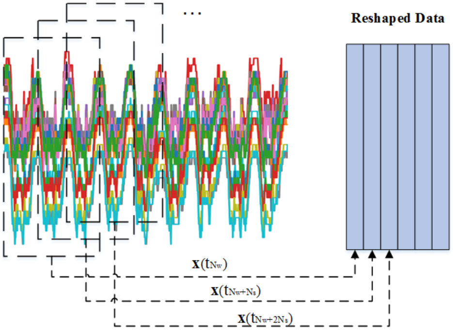
With a $P\times{N_{w}}$ (${N_{w}}\leq T$) window moving on ${\bf D}$ at the step size $N_{s}$, a series of data segments are generated. For example, at the sampling time $t_{j}$, the generated data segment is

$$\begin{aligned} {{\bf D}}(t_{j})=\left({{{\bf d}}(t_{j-{N_{w}}+1}),{{\bf d}}(t_{j-{N_{w}}+2}),\cdots,{{\bf d}}(t_{j})}\right)\end{aligned},$$

(1)

where ${{\bf d}}(t_{k})={({d_{1},d_{2},\cdots,d_{P}})}^{H}$ ($t_{j-{N_{w}}+1}\leq t_{k}\leq t_{j}$) is the sampling data at time $t_{k}$. For the data segment at the sampling time $t_{j}$, we reshape it into a column vector denoted as ${\bf x}_{t_{j}}\in\mathbb{R}^{P{N_{w}}\times 1}$. Thus, the spatio-temporal data matrix is reformulated as ${{\bf D}}=[{\bf x}({t_{N_{w}}});{\bf x}({t_{{N_{w}}+N_{s}}});{\bf x}({t_{{N_{w}}+2\times N_{s}}});\cdots]$, which is shown in Figure 1.

To reduce the calculation error and improve the convergence speed of training BiGANs in the subsequent feature learning process, we normalize $\bf x$ into $\tilde{\bf x}$ by

$$\begin{aligned} {\tilde{x}_{i}}=\frac{{{x_{i}}-\min({{\bf{x}}})}}{{\max({{\bf{x}}})-\min({{\bf{x}}})}}\end{aligned},$$

(2)

where ${\tilde{x}_{i}}(i=1,2,\cdots,PN_{w})$ is the normalized value in the range $[0,1]$, $\min({{\bf{x}}})$ and $\max({{\bf{x}}})$ respectively denote the minimum and maximum value of $\bf x$.

BiGANs, train a generative model $G$ to capture the distribution of the sample data, a discriminative model $D$ to distinguish the real samples from the generated ones as accurately as possible, and an encoding model $E$ to project sample data back into the latent space. Feature representations learned by the encoding model can depict the rich structure information of the sample data well, which can be used for other auxiliary problems. The framework of BiGANs is shown in Figure 2.

The generative model $G$, also called generator, is composed of multi-layer networks. For convenience, we assume it’s a three-layer network, i.e., the input layer, one hidden layer and the output layer. Data transition from the input layer to the output layer can be denoted as in Equation (3) and (4).

$$\begin{aligned} {\bf h}_{g}={S_{h}}({\bm{W}}_{h}{{\bf z}}+{{\bm{b}}_{h}})\end{aligned},$$

(3)

$$\begin{aligned} G({\bf z})={S_{g}}({\bm{W}}_{g}{{\bf h}_{g}}+{{\bm{b}}_{g}})\end{aligned},$$

(4)

where $\bf z$ is the input data sampled from a simple latent distribution (gaussian, uniform, exponential, etc), ${\bf h}_{g}$ is the output of the hidden layer in $G$, ${\bm{W}}_{h}$ is the weight matrix between the input layer and the hidden layer and ${\bm{W}}_{g}$ is the weight matrix between the hidden layer and the output layer. To avoid gradient vanishing in training multi-layer $G$, as proposed in [10], ${\bm{W}}_{h}$ and ${\bm{W}}_{g}$ can be initialized by using an uniform distribution

$$\begin{aligned} U[-\frac{\sqrt{6}}{\sqrt{{M_{i}}+{M_{i+1}}}},\frac{\sqrt{6}}{\sqrt{{M_{i}}+{M_{i+1}}}}]\end{aligned},$$

(5)

where $M_{i}$ and $M_{i+1}$ are the fan-in and fan-out of the units in the $i-$th layer, $U[x1,x2]$ denotes the uniform distribution supported by $x1$ and $x2$. ${\bm{b}}_{h}$ and ${\bm{b}}_{g}$ are the bias vectors, which can be initialized as small random values or 0. $S_{h}$ and $S_{g}$ are activation functions, such as sigmoid function, or tanh function, or rectified linear units (ReLu) first proposed in [11]

$$\begin{aligned} {s(a)}=max(0,a)\end{aligned},$$

(6)

or leaky ReLu (LReLu) proposed in [12][13]

$$\begin{aligned} {s(a)}=max(0,a)-\beta\times min(0,a)\end{aligned}.$$

(7)

The parameter $\beta$ in Equation (7) represents the slope of the leak. Compared with ReLu, the LReLu can keep a small gradient even though the unit is saturated. The output $G({\bf z})$ is the generated sample, which has the same size with the real data sample.

The encoding model $E$, also called encoder, is stacked with multi-layer neural networks. Assuming an encoder with only two-layer networks, i.e., the input layer and one hidden layer, data transition from the input data $\tilde{\bf x}$ to the hidden units is called encoding, which is defined as

$$\begin{aligned} E({\tilde{\bf x}})={S_{e}}({\bm{W}}_{e}{\tilde{\bf x}}+{{\bm{b}}_{e}})\end{aligned},$$

(8)

where ${\bm{W}}_{e}$ is the weight matrix between the input layer and the hidden layer, which can be initialized through Equation (5). ${\bm{b}}_{e}$ is the bias vector initialized with small random values or 0, and $S_{e}$ is the activation function. The output $E({\tilde{\bf x}})$ can be considered as the feature representations of the real sample data ${\tilde{\bf x}}$ in the latent space.

The discriminative model $D$, called discriminator, is also with multi-layer network structure, i.e., the input layer, multiple hidden layers, and the output layer. It takes the combination of the sample data and its latent features as the input $\bf y$ (i.e., ${\bf y}=[G({\bf z}),{\bf z}]$ or ${\bf y}=[{\tilde{\bf x}},E({\tilde{\bf x}})]$), and outputs $D({\bf y})\in[0,1]$ to represent the probability that $\bf y$ is from the real sample rather than the generated one. Considering a discriminator with three-layer network, the discriminative process can be denoted as in Equation (9) and (10).

$$\begin{aligned} {\bf h}_{d}={S_{h}}({\bm{W}}_{h}{{\bf y}}+{{\bm{b}}_{h}})\end{aligned},$$

(9)

$$\begin{aligned} D({\bf y})={S_{d}}({\bm{W}}_{d}{{\bf h}_{d}}+{{\bm{b}}_{d}})\end{aligned},$$

(10)

where $S_{h}$ and $S_{d}$ are the activation functions, ${\bm{W}}_{h}$ and ${\bm{W}}_{d}$ are the weight matrices initialized through Equation (5), ${\bm{b}}_{h}$ and ${\bm{b}}_{d}$ are the bias vectors initialized with small random values or 0, and ${\bf h}_{d}$ represents the output of the hidden layer in $D$.

Let $p_{\bf X}$ be the distribution of the real data $\bf x$ for $\bf x\in{\Phi_{\bf X}}$ (e.g. data segments), $p_{\bf Z}$ be the distribution of the sampled data $\bf z$ in $G$ for $\bf z\in{\Phi_{\bf Z}}$. In BiGANs, we train $D$ to maximize the probability of distinguishing the real samples from the generated ones (i.e., maximizing $\log D(\tilde{\bf x},E(\tilde{\bf x}))$), train $G$ to minimize the probability of $D$ making correct distinctions (i.e., minimizing $\log(1-D(G(\bf z),{\bf z}))$, and simultaneously train $E$ to map the real data $\tilde{\bf x}$ into the latent space of $G$ (i.e., introducing $p_{E}({\bf z}|{\bf x})$. Thus, the objective function of training BiGANs can be defined as [9]

$$\begin{aligned} \min\limits_{G,E}\max\limits_{D}V(D,E,G)\end{aligned},$$

(11)

where

$$\begin{aligned} V(D,E,G)&=\mathbb{E}_{{\bf x}\sim p_{\bf X}}\log D(\tilde{\bf x},E(\tilde{\bf x}))\\ &+\mathbb{E}_{{\bf z}\sim p_{\bf Z}}\log(1-D(G(\bf z),{\bf z}))\end{aligned}.$$

(12)

Considering the large number of parameters in BiGANs, it is mandatory to introduce an regularization technique to prevent the overfitting problem. Dropout, first proposed in [14], addresses this problem by introducing randomness, i.e., dropping out the units in the hidden layers with a fixed probability, such as 0.2. The minimax objective function in Equation (11) can be optimized by using stochastic gradient descent (SGD) based techniques, such as adaptive subgradient (AdaGrad) method [15], root mean square prop (RMSprop) alogithm [16], adaptive moment (Adam) estimation [17], etc. Here, we choose Adam as the optimization algorithm, which combines the advantages of AdaGrad and RMSprop, i.e., sparse gradients, online and non-stationary settings.

In practice, the objective function in Equation (11) may not provide sufficient gradients for $G$ to learn well, because $D$ can clearly distinguish real sample from the generated one early in learning and this will easily lead to $\log(1-D(G(\bf z),{\bf z}))$ to saturate. Therefore, we can train $G$ by maximizing $\log(D(G(\bf z),{\bf z}))$ instead of minimizing $\log(1-D(G(\bf z),{\bf z}))$. Theoretical results in [9] show the objective function $V(D,E,G)$ achieves its global minimum value $-\log 4$ if and only if $[G({\bf z}),{\bf z}]$ and $[{\tilde{\bf x}},E({\tilde{\bf x}})]$ have the same distribution (i.e., $p_{G({\bf z}),{\bf z}}=p_{{\tilde{\bf x}},E({\tilde{\bf x}})}$).

The process of feature learning is training BiGANs, i.e., obtaining the optimal parameters $\theta_{D},\theta_{E},\theta_{G}$ by minimaximizing the objective function in Equation (11). Here, $\theta_{D},\theta_{E}$ and $\theta_{G}$ denote the corresponding parameters (i.e., $\bm{W}$ and $\bm{b}$) in $D,E$ and $G$. When the network almost converges (i.e., $G\approx E^{-1}$), the features output by the encoder can be considered as the latent representations of the real data in the generator’s space, which can be used for the subsequent anomaly detection task.

Based on the features extracted through BiGANs for each data segment, a high-dimensional statistical index for them is calculated to indicate the data behavior. For example, at the sampling time $t_{j}$, the statistical index for the learned features ${\bm{f}}(t_{j})$ is calculated as

$$\begin{aligned} \mathcal{N}_{\phi}\left({t_{j}}\right)=\sum\limits_{|{\emph{f}}_{r}(t_{j})|>median(|{\bm{f}}(t_{j})|)}{\phi\left(|{{{\emph{f}}_{r}(t_{j})}}|\right)}\end{aligned},$$

(13)

where ${{{\emph{f}}_{r}(t_{j})}}\in{\bm{f}}(t_{j})$. The test function $\phi(\cdot)$ makes a linear or nonlinear mapping for the features, which can be chebyshev polynomial (CP), information entropy (IE), likelihood radio function (LRF) or wasserstein distance (WD). Detailed information about the test functions can be found in [18]. $\mathcal{N}_{\phi}$ is a complex function of the extracted features, which will be further discussed in Section IV-A.

Considering random weight initialization and dropout enforces randomness during the adversarial feature learning, the average value of the objective function in continuous $n$ iterations is calculated to judge whether terminating the training. For example, for the $i-$th iteration, the average value is calculated as

$$\begin{aligned} V_{\text{avg}}(D,E,G)=\frac{1}{n}\sum\limits_{l=i-n+1}^{i}V_{l}(D,E,G)\end{aligned},$$

(14)

where $V_{l}(D,E,G)$ is the calculated objective function value in the $l-$th ($l=i-n+1,\cdots,i$) iteration, and $V_{\text{avg}}(D,E,G)$ denotes the average value for continuous $n$ iterations. Here, the simple averaging method in ensemble learning is used. For each iteration, one network learning model is built and outputs $V_{l}(D,E,G)$. Thus, in continuous $n$ iterations, the average result $V_{\text{avg}}(D,E,G)$ for $n$ learning models is more accurate in judging whether to terminate the training than simply using the output $V_{i}(D,E,G)$ in the last iteration, because the former is more stable and reliable for reducing the error caused by randomness and the risk of network falling into local optimum. The procedure for anomaly detection based on BiGANs is summarized as in Algorithm 1.

As illustrated in Figure 3, one feeder line in the partial distribution network consists of branch lines and substations with distribution transformers. On the low voltage side of each distribution transformer, one online monitoring sensor is installed, through which we can obtain multiple measurements, such as three-phase voltages (i.e.,$u_{a},u_{b},u_{c}$). Here, we choose $u_{a},u_{b},u_{c}$ at the sampling time $t_{j}$ to formulate a data vector ${{\bf{d}}(t_{j})}={\left[{{{u}}_{aj}^{\left(1\right)},{{u}}_{bj}^{\left(1\right)},{{u}}_{cj}^{\left(1\right)},\cdots,{{u}}_{aj}^{\left(m\right)},{{u}}_{bj}^{\left(m\right)},{{u}}_{cj}^{\left(m\right)}}\right]^{H}}$, where $m$ denotes the number of sensors installed on the feeder. Let $P=3m$, for a series of time $T$, we can obtain a spatio-temporal data matrix ${\bf D}=[{\bf d}(t_{1}),{\bf d}(t_{2}),\cdots,{\bf d}(t_{T})]\in{\mathbb{R}^{P\times T}}$. It is noted that, by stacking the voltage measurements together, the formulated spatio-temporal data matrix contains rich information on the operating state of the feeder line.

The anomaly detection result can indicate the operating states of the feeder lines in distribution networks. Here, it is used as the basis for assessing the operational risks. For a series of time $T^{\prime}$, the anomaly index $\mathcal{N}_{\phi}$ for each data segment is calculated, size of which is $\frac{T^{\prime}}{N_{s}}$. We first standardize $\mathcal{N}_{\phi}$ by

$$\begin{aligned} {\hat{\mathcal{N}_{\phi}}}=\frac{{\mathcal{N}_{\phi}}-\mu({\mathcal{N}_{\phi}})}{\sigma({\mathcal{N}_{\phi}})}\end{aligned},$$

(15)

where $\mu({\mathcal{N}_{\phi}})$ and $\sigma({\mathcal{N}_{\phi}})$ are the sample mean and sample standard deviation of ${\mathcal{N}_{\phi}}$ in a series of time $T^{\prime}$.

Considering the sample size $\frac{T^{\prime}}{N_{s}}$ is sometimes small, here, $\hat{\mathcal{N}_{\phi}}$ is assumed to follow a student’s t-distribution with $\frac{T^{\prime}}{N_{s}}-1$ degrees of freedom, i.e., $\hat{\mathcal{N}_{\phi}}\sim t(\frac{T^{\prime}}{N_{s}}-1)$. According to the central limit theorem, the confidence level $1-\alpha$ for the population mean $\mu$ of $\hat{\mathcal{N}_{\phi}}$ is defined as

$$\begin{aligned} 1-\alpha=P\{{\mu(\hat{\mathcal{N}_{\phi}})-t_{\frac{\alpha}{2}}{\frac{\sigma(\hat{\mathcal{N}_{\phi}})}{\sqrt{\frac{T^{\prime}}{N_{s}}}}}}<\mu<{\mu(\hat{\mathcal{N}_{\phi}})+t_{\frac{\alpha}{2}}{\frac{\sigma(\hat{\mathcal{N}_{\phi}})}{\sqrt{\frac{T^{\prime}}{N_{s}}}}}}\}\end{aligned},$$

(16)

where $\mu(\hat{\mathcal{N}_{\phi}})$ and $\sigma(\hat{\mathcal{N}_{\phi}})$ are the sample mean and sample standard deviation of $\hat{\mathcal{N}_{\phi}}$ with $\mu(\hat{\mathcal{N}_{\phi}})=0$ and $\sigma(\hat{\mathcal{N}_{\phi}})=1$, $t_{\frac{\alpha}{2}}$ is the upper $\frac{\alpha}{2}$ critical value for the t distribution with $\frac{T^{\prime}}{N_{s}}-1$ degrees of freedom, and $P\{\cdot\}$ is the probability operator. Thus, the confidence interval of level $1-\alpha$ is simplified as $[-t_{\frac{\alpha}{2}}{\frac{1}{\sqrt{\frac{T^{\prime}}{N_{s}}}}},t_{\frac{\alpha}{2}}{\frac{1}{\sqrt{\frac{T^{\prime}}{N_{s}}}}}]$, and the p value for the interval critical values is equal to $\frac{\alpha}{2}$. For a given $\hat{\mathcal{N}_{\phi}}$, the corresponding p value can be obtained by the t distribution table. For example, let ${\hat{\mathcal{N}_{\phi}}}=2.650$ and $\frac{T^{\prime}}{N_{s}}-1=13$, then the p value is $1\%$.

To further quantify the operational risks of feeder lines in distribution networks, we classify the operational risk levels into emergency, high risk, preventive and normal according to the defined intervals of the confidence level $1-\alpha$ for the population mean of $\hat{\mathcal{N}_{\phi}}$, which is shown in Table I. Thus, for a calculated $\hat{\mathcal{N}_{\phi}}$, we can judge the operational risk level by comparing the p value with the corresponding interval of $\frac{\alpha}{2}$: the smaller the p value, the higher the risk level.

Here, “emergency” means a feeder line operates in abnormal state and serious faults may happen at any time. If one feeder is diagnosed as in emergency state, it will be further analyzed. “High risk” denotes a feeder line is of high risk in suffering from faults, which deserves special attention. “Preventive” means a feeder line operates in normal state, but it is not safe and should be watched for a period of time. “Normal” denotes a feeder line is in healthy state. By using Table I, the operational risks of feeders are quantified, which offer references for operators to make safety assessments.

Based on the research above, an unsupervised risk assessment approach in distribution networks is proposed. The steps of the approach are shown as follows.

The operational risk assessment approach proposed is driven by the online monitoring data and based on adversarial feature learning theory. Step 1 is conducted for the formulation of a spatio-temporal data matrix for each feeder. In Step 2, the data matrix is partitioned into a series of data segments by using a moving window method. Step 3 is the adversarial feature learning process for each data segment, in which no assumptions or simplifications are made for the underlying structure of the real data. Step 4$\sim$6 are conducted for the operational risk assessment based on the central limit theorem. The proposed approach is practical for online analysis when the last sampling time is considered as the current time.

The synthetic data was sampled from the simulation results of the IEEE 118-bus test system [19]. In the simulations, a sudden change of the active load at one bus was considered as an anomaly signal and a little white noise was introduced to represent random fluctuations.

1) Case Study on $z-$sampling Distribution: In BiGANs, $z$ represents the input data of the generative model $G$, which is sampled from a simple distribution, such as uniform distribution, gaussian distribution, exponential distribution, etc. In this case, we will explore whether $z-$sampling distribution affects the proposed approach’s performance. The synthetic data set contained 118 voltage measurements for sampling 500 times. An assumed step signal was set for bus 20 during $t_{s}=251\sim 255$ and others stayed unchanged, which was shown in Table II.

The other involved parameters were set as follows:
– The moving window’s size $P\times N_{w}$: $118\times 10$;
– The moving step size $N_{s}$: $10$;
– The number of layers for $D$/$E$/$G$: $5$;
– The number of neurons in each hidden layer of $D$:

$768,320,256$;
– The number of neurons in each hidden layer of $E$:

$768,320,256$;
– The number of neurons in each hidden layer of $G$:

$256,320,768$;
– The feature size: 64;
– The number of steps $m$ applied to $D$: 1;
– The number of iterations $n$ to calculate $V_{\text{avg}}(D,E,G)$: 10;
– The initial learning rate $\eta$: 0.0002;
– The slope of the leak $\beta$ in LReLu: 0.2;
– The dropout coefficient: 0.1;
– The required approximation error $\varepsilon$: 0.0001;
– The test function $\phi(\lambda)$: $-\lambda$ln$(\lambda)$.

For exploring the effect of $z-$sampling distribution on the performance of the proposed approach, the statistical indices with $z$ sampled from uniform distribution (i.e., $z\sim U(0,1)$), gaussian distribution (i.e., $z\sim N(0,1)$) and exponential distribution (i.e., $z\sim E(1)$) were respectively calculated and the corresponding $\mathcal{N}_{\phi}-t$ curves were plotted in Figure 4. It can be observed that the assumed anomaly signal can be detected when $z$ is sampled from any distribution. Meanwhile, for the $\mathcal{N}_{\phi}-t$ curves, the p values of $\hat{\mathcal{N}_{\phi}}$ corresponding to the anomaly point were calculated, results of which were $0.0005\%$, $0.0005\%$, $0.0005\%$, respectively. It can be concluded that the detection performance of the proposed approach is almost not affected by the assumption of $z-$sampling distribution.

In the experiment, the synthetic data set were partitioned into $50$ data segments and $\mathcal{N}_{{\phi},l}(l=1,\cdots,n=10)$ were generated for each data segment. In order to explore the shape of the sampling distribution of the anomaly index corresponding to different $z-$sampling distribution, the probability density function (PDF) curves of $\hat{\mathcal{N}_{\phi}}$ with outliers (the values corresponding to the anomaly point) dropped are plotted in Figure 5. It can be observed that the sampling distribution of $\hat{\mathcal{N}_{\phi}}$ is approximately normal when the degrees of freedom are large, regardless of $z-$sampling distribution. It validates our assumption in Section III-B that $\hat{\mathcal{N}_{\phi}}$ follows a t distribution.

2) Case Study on Model Depth: Since $D,E$ and $G$ in BiGANs are composed of multi-layer network, in this case, we will explore how the model depth (i.e., the number of layers in $D$/$E$/$G$) affects the proposed approach’s performance. The generated data set in Case 1) was used in this case, and $z$ was sampled from standard gaussian distribution, i.e., $z\sim N(0,1)$. The other involved parameters were set the same as in Case 1). For illustrating the effect of model depth on the performance of the proposed approach, the anomaly indices corresponding to different model depth were calculated and normalized into $[0,1]$, which was shown in Figure 6.

It can be observed that the assumed anomaly signal can be detected for different model depth (i.e., $depth=3,4,5,6$). Meanwhile, for the $\mathcal{N}_{\phi}-t$ curves, the p values of $\hat{\mathcal{N}_{\phi}}$ corresponding to the anomaly point were calculated, results of which were $0.1815\%$, $0.0005\%$, $0.0005\%$, $0.0030\%$, respectively. It shows that the best anomaly detection performance is achieved when the model depth is $4$ or $5$. Furthermore, the effect of model depth on the convergence rate in training BiGANs is illustrated in Figure 7. Considering the performance and efficiency comprehensively, the model depth is set as $5$ in the subsequent experiments.

3) Case Study on Feature Size: In this case, the effect of feature size on the performance of the proposed approach is explored. The generated data set in case 1) was used in this case, and the model depth was set to be $5$. The other involved parameters were set the same as in Case 1). The anomaly indices corresponding to different feature size were calculated and normalized into $[0,1]$, which was shown in Figure 8.

It can be observed that the assumed anomaly signal can be detected for different feature size (i.e., $size=20,40,60,80,100$). For the $\mathcal{N}_{\phi}-t$ curve, the p values of $\hat{\mathcal{N}_{\phi}}$ corresponding to the anomaly point were calculated and the results were $0.0010\%$, $0.0005\%$, $0.0005\%$, $0.0005\%$, $0.0115\%$, respectively. It can be concluded that: 1) when the feature size is small (such as 20 or 40), the proposed approach is sensitive to the anomaly signal, but it is vulnerable to random fluctuations; 2) with the increase of feature size, the proposed approach becomes less sensitive to the anomaly signal and more robust to random fluctuations. In the experiment, we note that large feature size will lead to a slow convergence rate in training BiGANs. Therefore, a moderate feature size is often selected empirically.

In this section, the online monitoring data obtained from a distribution network in Hangzhou city of China is used to validate the proposed approach. The distribution network contains $200$ feeder lines with $8000$ distribution transformers. The online monitoring data were sampled every 15 minutes. Anomaly time and type for each feeder line were recorded during the operation. In the following cases, three-phase voltages were chosen as the measurement variables to formulate the data matrices. Voltage violation and disturbance were considered as the risk items.

1) Case Study on Voltage Violation: Voltage violation is an common anomaly type in distribution networks, which increases the operational risks of the networks. It contains two aspects, i.e., exceeding the upper limit or the lower limit. In this case, we assess the operational risk of one feeder line suffering from voltage violation to validate the proposed approach. The feeder, with branch lines and substations, contained $15$ distribution transformers in total. The online monitoring data were sampled from 2017/3/1 00:00:00 to 2017/3/14 23:45:00, thus a $45\times 1344$ data matrix was formulated. The data with anomaly time and type labelled are shown in Figure 9. The involved parameters are set as follows:
– the moving window’s size $P\times N_{w}$: $45\times 96$;
– the moving step size $N_{s}$: $96$;
– the model depth: $5$;
– the number of neurons in each hidden layer of $D$:

$1660,960,320$;
– the number of neurons in each hidden layer of $E$:

$1660,960,320$;
– the number of neurons in each hidden layer of $G$:

$320,960,1660$;
– the feature size: $64$;
– the number of steps $m$ applied to $D$: $1$;
– the number of iterations $n$ to calculate $V_{\text{avg}}(D,E,G)$: $5$;
– the initial learning rate $\eta$: $0.0001$;
– the slope of the leak $\beta$ in LReLu: $0.2$;
– the dropout coefficient: $0.2$;
– the required approximation error $\varepsilon$: $0.0001$;
– the test function $\phi(\lambda)$: $-\lambda$ln$(\lambda)$.

Figure 10 shows the anomaly detection results when $z$ is sampled from uniform distribution, gaussian distribution, exponential distribution, respectively. From the $\mathcal{N}_{\phi}-t$ curves, we can obtain:

I. The value of $\mathcal{N}_{\phi}$ on March 13th is significantly smaller than those on other days, which indicates anomaly occurred on March 13th. The PDFs of the extracted features corresponding to March 13th and other days (such as March 1st) are shown in Figure 11. It can be observed that the PDFs of the extracted features are different when the feeder operates in different states, i.e., the PDF of the extracted features in normal operating state is more centered.

II. The p values of $\hat{\mathcal{N}_{\phi}}$ corresponding to the anomaly time for different $z-$sampling distribution were calculated, results of which were $0.1850\%$, $0.2005\%$, $0.2195\%$, respectively. It validates the performance of the proposed approach is almost not affected by the assumption $z-$sampling distribution.

III. The calculated p values of $\hat{\mathcal{N}_{\phi}}$ on March 13th are smaller than $\frac{\alpha}{2}=\frac{1-97.5\%}{2}=1.25\%$, which indicates the feeder operates in emergency state and it needs to be further analyzed.

2) Case Study on Voltage Disturbance: Voltage disturbance is an complex anomaly type in distribution networks, which is random in magnitude and could involve sporadic bursts as well. It may be caused by short circuit fault, sudden load change, or connection of distribution generation, etc. In this case, the performance of the proposed approach is tested by assessing the operational risk of one feeder line suffering from voltage disturbance. The feeder contained $7$ distribution transformers and the online monitoring data were sampled during 2017/3/1 00:00:00 $\sim$ 2017/3/14 23:45:00, thus a $21\times 1344$ data matrix was formulated. The data with anomaly time and type labelled are shown in Figure 12. The moving window’s size was $21\times 96$, the number of neurons in each hidden layer of $D$/$E$ were $1120,672,256$, and the number of neurons in each hidden layer of $G$ were $256,672,1120$. The other parameters were set the same as in the above case.

Figure 13 shows the anomaly detection results corresponding to different $z-$sampling distributions. From the $\mathcal{N}_{\phi}-t$ curves, we can obtain:

I. The value of $\mathcal{N}_{\phi}$ on March 9th is smaller than those on other days, which indicates the latent anomaly is accurately detected. The PDFs of the extracted features corresponding to abnormal and normal feeder operating states are shown in Figure 14. It can be observed that, the PDF of the extracted features in normal operating state is more centered.

II. For each $\mathcal{N}_{\phi}-t$ curve, the p values corresponding to the anomaly time were calculated, results of which were $0.235\%$, $0.196\%$, $0.353\%$, respectively. It also validates the performance of the proposed approach is almost not affected by the assumption of $z-$sampling distribution.

III. The calculated p values of $\hat{\mathcal{N}_{\phi}}$ on March 9th is smaller than $\frac{\alpha}{2}=1.25\%$, which indicates the feeder operates in emergency state and it deserves to be further analyzed.

3) Comparison with Other Existing Approaches: We further compare the proposed approach with other existing approaches in accuracy and efficiency by assessing the operational risks of feeder lines suffering from anomalies. Here, the risk levels in Table I are simplified as abnormal (emergency state) and normal (the other states). Anomaly detection techniques based on deep autoencoders (DAE) [20][21], principal component analysis (PCA) [2], spectrum analysis (SPA) [18], or threshold analysis (THA) [22] have been well studied. In order to make a full comparison with the other existing techniques, we analyzed $180$ feeder lines with $250$ anomaly records during 2017/3/1 00:00:00 $\sim$ 2017/4/30 23:45:00. Here, voltage violation and fluctuation were considered as anomaly items. For DAE, PCA, and SPA, the moving window’s size was $P\times 96$, the moving step size was $96$ and the test function was $\phi(\lambda)=-\lambda$ln$(\lambda)$. For THA, the anomaly index was defined as

$$\begin{aligned} P(\text{A})=\frac{\sum\limits_{j=1}^{n(\text{A})}t(\text{A})_{j}}{T^{\prime}}\end{aligned},$$

(17)

where $T^{\prime}$ is the total number of sampling times, $t(\text{A})_{j}$ is the duration for each abnormal state (i.e., the voltage exceeds the upper or lower limit), $n(\text{A})$ is the number of abnormal states, and $P(\text{A})\in[0,1]$. In the experiments, the optimal parameters involved in each detection approach were tested, and they were set as in Table III.

In order to compare the detection performances of different approaches, $true\;detection\;rate\;(TDR)$ and $false\;alarm\;rate\;(FAR)$ are used to measure the performance of each method. The $TDR$ and $FAR$ are defined as

$$\begin{aligned} &TDR=\frac{N_{cr}}{N_{gt}}\\ &FAR=\frac{N_{al}-N_{cr}}{N_{al}}\end{aligned},$$

(18)

where $N_{cr}$ is the number of anomalies that are correctly detected, $N_{gt}$ denotes the number of ground-truth anomalies, and $N_{al}$ is the number of all detected alarms. The higher the $TDR$ and the smaller the $FAR$, the better detection performance of one approach. Meanwhile, in order to compare the efficiency of different approaches, the $average\;calculation\;time\;(ACT)$ for each $96$ sampling times (i.e., the moving window’s width) was counted. The experiments were conducted on a server with $2.60$ GHz central processing unit (CPU) and $8.00$ GB random access memory (RAM). The comparison results are shown in Table IV.

It can be observed that the proposed BiGANs-based approach has the highest $TDR$ and the smallest $FAR$, which indicates it outperforms DAE, PCA, SPA and THA in anomaly detection performance. The reasons are:

• •

  THA uses the simple statistical features that often are not well generalized, which makes it impossible to detect the latent anomalies.

• •

  SPA makes an assumption that the input data follows a certain distribution and the entries of the data matrix are independently and identically distributed. Besides, SPA is an anomaly detection approach based on correlation analysis, which is not sensitive to the amplitude variation of the data.

• •

  PCA is a linear dimension reduction approach and the optimal parameter measuring the contribution rate of top $k$ eigenvalues is hard to find for all data segments.

• •

  DAE is a nonlinear generalization of PCA and it is vulnerable to the random fluctuations for the reason of simple network structure and learning algorithm.

The proposed approach overcomes the shortcomings of the other existing approaches by using complex $D,E,G$ to learn the features of the input data in an adversarial way. Meanwhile, it is noted that the proposed approach has the highest $ACT$ (i.e., $4.235$s) for the reason of complex network structure and learning algorithm, which indicates the worst detection efficiency compared with the other approaches. However, considering the online monitoring data in the researched network is sampled every 15 minutes, the proposed approach is practical for the online operational risk analysis. Moreover, with the development of graphics processing unit (GPU) and field-programmable gate array (FPGA) techniques, the computational efficiency will be improved greatly.

References

- [1] M. R. Jaafari Mousavi, “Underground distribution cable incipient fault diagnosis system,” 2007.
- [2] L. Xie, Y. Chen, and P. R. Kumar, “Dimensionality reduction of synchrophasor data for early event detection: Linearized analysis,” IEEE Trans. Power Syst., vol. 29, no. 6, pp. 2784–2794, Nov. 2014.
- [3] A. C. Adewole and R. Tzoneva, “Fault detection and classification in a distribution network integrated with distributed generators,” in IEEE Power and Energy Society Conference and Exposition in Africa: Intelligent Grid Integration of Renewable Energy Resources (PowerAfrica), Jul. 2012, pp. 1–8.
- [4] M. Wu and L. Xie, “Online detection of low-quality synchrophasor measurements: A data-driven approach,” IEEE Trans. Power Syst., vol. 32, no. 4, pp. 2817–2827, Jul.
- [5] M. Pignati, L. Zanni, P. Romano, R. Cherkaoui, and M. Paolone, “Fault detection and faulted line identification in active distribution networks using synchrophasors-based real-time state estimation,” IEEE Trans. Power Del., vol. 32, no. 1, pp. 381–392, Feb. 2017.
- [6] A. Ghaderi, H. A. Mohammadpour, H. L. Ginn, and Y.-J. Shin, “High-impedance fault detection in the distribution network using the time-frequency-based algorithm,” IEEE Trans. Power Del., vol. 30, no. 3, pp. 1260–1268, Jun. 2015.
- [7] L. Chu, R. C. Qiu, X. He, Z. Ling, and Y. Liu, “Massive streaming pmu data modeling and analytics in smart grid state evaluation based on multiple high-dimensional covariance tests,” IEEE Trans. Big Data, vol. 4, no. 1, pp. 55–64, Mar. 2018.
- [8] I. J. Goodfellow, J. Pouget-Abadie, M. Mirza, B. Xu, D. Warde-Farley, S. Ozair, A. Courville, and Y. Bengio, “Generative adversarial nets,” in Proc. Adv. Neural Inform. Process. Syst., 2014, pp. 2672–2680.
- [9] J. Donahue, P. Krähenbühl, and T. Darrell, “Adversarial feature learning,” in Proc. Int. Con. Learn. Rep.
- [10] X. Glorot and Y. Bengio, “Understanding the difficulty of training deep feedforward neural networks,” in Proc. 13th Int. Conf. Artf. Intell. Stat., 2010, pp. 249–256.
- [11] V. Nair and G. E. Hinton, “Rectified linear units improve restricted boltzmann machines,” in Proc. 27th Int. Con. Mach. Learn., 2010, pp. 807–814.
- [12] A. L. Maas, A. Y. Hannun, and A. Y. Ng, “Rectifier nonlinearities improve neural network acoustic models,” in Proc. 30th Int. Con. Mach. Learn., vol. 30, no. 1, 2013, p. 3.
- [13] B. Xu, N. Wang, T. Chen, and M. Li, “Empirical evaluation of rectified activations in convolutional network,” arXiv preprint arXiv:1505.00853, 2015. [Online]. Available: http://arxiv.org/abs/1505.00853
- [14] N. Srivastava, G. Hinton, A. Krizhevsky, I. Sutskever, and R. Salakhutdinov, “Dropout: a simple way to prevent neural networks from overfitting,” J. Mach. Learn. Res., vol. 15, no. 1, pp. 1929–1958, Jun. 2014.
- [15] J. Duchi, E. Hazan, and Y. Singer, “Adaptive subgradient methods for online learning and stochastic optimization,” J. Mach. Learn. Res., vol. 12, pp. 2121–2159, Jul. 2011.
- [16] T. Tieleman and G. Hinton, “Lecture 6.5-rmsprop, coursera: Neural networks for machine learning,” University of Toronto, Technical Report, 2012. [Online]. Available: https://www.cs.toronto.edu/ tijmen/csc321/slides/lecture_slides_lec6.pdf
- [17] D. P. Kingma and J. Ba, “Adam: A method for stochastic optimization,” 2015.
- [18] X. Shi, R. Qiu, X. He, L. Chu, and Z. Ling, “Anomaly detection and location in distribution networks: A data-driven approach,” arXiv preprint arXiv:1801.01669, 2018. [Online]. Available: https://arxiv.org/abs/1801.01669
- [19] R. D. Zimmerman, C. E. Murillo-Sanchez, and R. J. Thomas, “Matpower: Steady-state operations, planning, and analysis tools for power systems research and education,” IEEE Trans. Power Syst., vol. 26, no. 1, pp. 12–19, Feb 2011.
- [20] W.-H. Lee, J. Ortiz, B. Ko, and R. Lee, “Time series segmentation through automatic feature learning,” arXiv preprint arXiv:1801.05394, 2018. [Online]. Available: https://arxiv.org/abs/1801.05394
- [21] P. P. Barbeiro, H. Teixeira, J. Krstulovic, J. Pereira, and F. Soares, “Exploiting autoencoders for three-phase state estimation in unbalanced distributions grids,” Elect. Power Syst. Res., vol. 123, pp. 108–118, Jun. 2015.
- [22] T. Xiao, W. Pei, H. Ye, G. Niu, H. Xiao, and Z. Qi, “Operation risk assessment of distribution network considering time dependence correlation coefficient,” J. Eng., vol. 2017, no. 13, pp. 2489–2495, Dec. 2017.