August 24, 2026
Scale-Invariant Two Component Dark Matter
1 and 2
1, , , 2
Abstract
We study a scale invariant extension of the standard model which can explain simultaneously dark matter and the hierarchy problem. In our set-up, we introduce a scalar and a spinor as two-component dark matter in addition to scalon field as a mediator. Interesting point about our model is that due to scale invariant conditions, compared to other two-component dark matter models, it has lower independent parameters. Possible astrophysical and laboratory signatures of two-component dark matter candidate are explored and it is shown that the most contribution of observed relic density of dark matter can be determined by spinor dark matter. Detectability of these dark matter particles is studied and the direct and invisible Higgs decay experiments are used to rule out part of the parameter space of the model. In addition, the dark matter self-interactions are considered and shown that their contribution saturate this constraint in the resonant regions.
1 Introduction
The standard Model (SM) has been established by the discovery of the Higgs boson and it can explain almost all of experimental results obtained until now. However there are a number of unanswered issues, either theoretical or experimental such as hierarchy problem, active neutrino masses, dark matter (DM) relic abundance, baryon asymmetry of the Universe, inflation in the early Universe, dark energy, and so on.
The existence of DM is inferred through crucial evidence such as galactic rotation curves, gravitational lensing, observations of merging galaxies, the cosmic microwave background (CMB) measurements, the large scale structure of the universe and the collision of the bullet clusters. As it is mentioned, there are still lack of experimental or observational evidences to precisely distinguish the correct particle physics model for DM physics.
To explain these issues a number of SM extensions such as supersymmetric standard model, technicolor and extra dimensions theories have been proposed. Despite the broad searches on the beyond SM at LHC, null results for beyond SM theories [1] shows that we have enough motivation to think about the alternative theories.
In almost all extended models, there are some additional particles, which usually have heavier masses compared to the electroweak (EW) scale. It is famous that the hierarchy problem arises from the fact that the negative Higgs mass term in Lagrangian of SM causes a quadratical divergent term proportional to the energy scale cut-off after including the quantum corrections. As an idea avoiding the hierarchy problem, classically scale invariant extensions provides an attractive framework [2]-[3]. In this picture, it is supposed that the tree-level Higgs mass is zero and in the quantum level the Higgs scalar gains a small mass from the radiative corrections. In fact, the Higgs mass term is the only term that breaks the classical scale invariance in the SM. Therefore by omitting the Higgs mass term from the SM potential, one can practically remove the hierarchy problem. In recent years, a lot of classically scale invariant models have been studied for the solution of the hierarchy problem and DM problem [4]. The possibility of other two-component models without concerning scale invariance have been extensively considered in literature [5]. Also the two-component DM has been studied in the context of scalar WIMP-like candidates [6]. Our goal in this paper is to address DM relic density and hierarchy problem by an extension of the scale invariant standard model (SISM) which contains a scalar and a spinor DM candidates.
The structure of this paper is as follows: in section 2, we introduce the scale invariant SM with two-component scalar and fermionic DM scenarios. In section 3, we study perturbativity constraints on two component scale-invariant DM. In section 4, we study freeze-out solutions to the relic density constraint. In section 5, we will study phenomenological aspects such as direct detection, indirect detection, self-interaction and invisible Higgs decay searches on parameters space of our model. The results are summarized in section 6. The decay rate and cross section formula for self-interaction of two component of DM are summarized in the appendix.
2 The model
In the SISM, before electroweak symmetry breaking all fields in the scale invariant sector of potential are massless. In the quantum level these fields gain mass from radiative Coleman-Weinberg symmetry breaking [3].
In this paper, we consider a scale-invariant extension of SM where Higgs mass term is absent, and the only term remaining in the Higgs potential will be . In order to have a scale invariant version of the SM possessing a Higgs doublet and other SM particles with their physical masses, at least two more scalars (singlet) must be added to the theory. The reason arises from this fact that in the absent of scalar DM, the square scalon mass was completely fixed and would be negative [2]. In order to satisfy this condition, we add three new fields, two scalars and one spinor in our model. All fields are singlets under SM gauge transformation and they are massless before spontaneous symmetry breaking. Two of these new fields, the scalar and the spinor , are assumed to be odd under a symmetry. These discrete symmetry guarantees the stability of the lightest odd particles. The other scalar field, , and all SM particles are even under the . Therefore under symmetry new fields transform as below:
| (1) |
The scalar part of the Lagrangian including the new fields is
| (2) |
where the most general scale-invariant potential which is renormalizable and invariant under gauge and -symmetry is
| (3) |
where , and are the doublet Higgs, the scalon and DM scalars, respectively.
The scale-invariant terms including new spinor field and its allowed interaction are given by
| (4) |
Since there are no allowed interaction terms in the Lagrangian including both odd fields, the heavier odd particle also turns out to be stable. Therefore, the model has an accidental symmetry that stabilizes the heavier odd particles and it contains two DM candidates.
In unitary gauge, , potential (3) becomes:
| (5) |
Minimum of potential (5) corresponds to fields vacuum expectation values. Necessary conditions for local minimum of are:
| (6) |
Eqs. (6) should hold for the fields vacuum expectation values. Note that we require the non-vanishing vacuum expectation values for the fields and so the scalar field remains stable because of the symmetry and thereby it can play the role of the DM. Therefore, we put in Eqs. (6):
| (7) |
We are looking for non trivial solution of (7) corresponding to non-vanishing vacuum expectation values for and . For non-zero and , Eq. (7) leads to
| (8) |
or simply:
| (9) |
Note that according to condition (8), the minimum of the potential term corresponding to vacuum expectation values of the fields is zero.
The filed breaks the electroweak symmetry with vacuum expectation value, , where . Thus the Higgs field after spontaneous symmetry breaking is given by:
| (10) |
As it was mentioned, the field also acquire a vacuum expectation value,
| (11) |
Notice that and mix with each other and can be rewritten by the mass eigenstates and as
| (12) |
where is the mixing angle. We identify with the SM-like Higgs observed at the LHC with a mass of about .
After the symmetry breaking, we have the following constraints:
| (13) |
where and are the masses of scalar and spinor DM after symmetry breaking, respectively. The field (scalon) is massless, and it can be shown that the elastic scattering cross section of DM off nuclei becomes drastically large and the model is immediately excluded by the direct detection experiments. The one-loop correction gives a mass to the massless eigenstate [2],[6]:
| (14) |
Notice that in the absence of scalar and fermionic DM, scalon mass was completely fixed by Higgs particle, the gauge boson and the top quark masses. For this reason, adding scalar field is inevitable. Moreover in the absence of additional scalar DM, the square scalon mass could be negative. Since and , Equation (14) leads to the following constraint on :
| (15) |
where
| (16) |
and which is the minimum of . Throughout this paper, we satisfy this condition.
According to (13), the model introduces only 5 free parameters including . In addition, the quartic coupling is irrelevant to the DM relic density. Therefore, the remaining free parameters are
| (17) |
It is remarkable that our model in comparison with other two-component DM models, has a much lower number of independent parameters and behaves like a single-component model. For this reason, it would be difficult to satisfy all theoretical and phenomenological constraints, simultaneously. This is the point that we encounter in the next sections. In the following, we examine perturbativity constraints on these four parameters.
3 Theoretical constraints
In this section, we discuss various constraints on the parameters of our model from theoretical considerations. These are furnished in the following. Perturbativity constraints on the parameters of the Lagrangian are
| (18) | ||||
| (19) |
Considering constraints (13) we have
| (20) | ||||
| (21) | ||||
| (22) | ||||
| (23) | ||||
| (24) |
One can easily show that Eq. (20) and Eq. (22) are established automatically. Constraint (21) leads to
| (25) |
where with (). The above equation, , is not a strong constraint on . However, it leads to a constraint on :
| (26) |
Regarding to Eq. (23)
| (27) |
and according to (15) we have,
| (28) |
Considering and , Eq. (28) leads to
| (29) |
where , , and . For (), there are two possibilities: first , so Eq. (29) is trivial and second , provides a constraint on :
| (30) |
Finally, we choose the following domains for the parameters space: (17)
| (31) | ||||
| (32) | ||||
| (33) | ||||
| (34) |
4 Relic abundance
The evolution of the number density of DM particles with time are governed by the Boltzmann equation. In this section, we compute the relic density for both DM candidates scalar and fermion in our model, at the present epoch. In general, the coupled Boltzmann equations for two-component DM and should be solved in order to compute the number density. The coupled Boltzmann equations for scalar and fermion are given by:
| (35) | |||||
| (36) | |||||
where denotes any SM particles. In all annihilations are taken into account except which does not affect the number density. By using , where is the photon temperature, as the independent variable instead of time and , one can rewrite the Boltzmann equations in terms of yield quantity, :
| (37) | |||||
| (38) | |||||
where is the Planck mass and is the effective numbers parameter. As it is seen in above equations, there are new terms in Boltzmann equations which describe the conversion of two DM particles into each other, . These two cross sections are also described by the same matrix element. Therefore, we expect and are not independent and their relation is:
| (39) |
The interactions between the two DM components take place by exchanging two scalar mass eigenstates and where the coupling of to is suppressed by . Therefore, it usually is the -mediated diagram that gives the dominant contribution. However, If one DM particle is heavier than the other one (16), the conversion of the heavier particle into the lighter one is relevant, . Thus, the contribution of in the relic density is dominant and the only option for annihilation of is via -mediated and -mediated diagrams into SM particles.
To solve numerically the two coupled Boltzmann differential equation, We have implemented the model into micrOMEGAs [7] (via LanHEP [8]). Since we have two stable DM particle, the DM constraint in this model reads
| (40) |
according to the data by Planck collaboration [9]. Another related quantity is the fraction of the DM density that is due to and denoted by and , respectively. So
| (41) |
Fig. 1 to 4 depict the relic density of fermionic and scalar DM as a function of the DM mass. According to these plots, the most contribution of DM relic density comes from fermionic DM, i.e., . Since, in our model scalar DM is always heavier than fermionic DM, in addition to annihilation to SM particles, it could also annihilate to fermionic DM particles. Therefore, its relic density is smaller than fermionic relic density.

Fig. 1 shows both DM relic densities as a function of for different values of . For any given value of the fermionic relic density features a double reduction at the and resonances (respectively at , and ). There is another reduction due to the opening of the annihilation channel. Note that, according to Eq. (14), itself depends on , and , so it is not an independent parameter. Therefore, in our relic density plots, it varies with and DM masses. In Fig. 1, scalar relic density does not vary dramatically with or . Note that is a determinative parameter in scalar DM annihilation to SM particles. On the other hand, annihilation of scalar DM to SM particles is more favorable than its annihilation to fermionic DM, because most SM particles are lighter than fermionic DM. Therefore, mostly depends on rather than . According to Eqs. (13) is given by
| (42) |
and for the given parameters in Fig. 1, is mostly determined by the first term of Eq. (42). Thus, it does not vary much with or .

In Fig. 2 DM relic densities are plotted versus for different values of . Similarly, for the given values of the fermionic relic density again features a double reduction at the and resonances (respectively at , and ). Obviously, in this plot at the first resonance is lighter than . For the scalar relic density, according to Eq. (42), larger leads to larger and therefore DM-SM interaction gets stronger which leads to smaller scalar relic density. Furthermore, now for , the second term of Eq. (42) can compete with the first term, and with growth of , will decrease. Due to this reduction, scalar DM-SM interaction becomes weaker and therefore increase with . For larger (for example again the first term of Eq. (42) dominates and increases less with .

Fig. 3 and 4 depict relic densities versus . In Fig. 3, for there is a single reduction in fermionic relic density around . This reduction corresponds to which is a resonance case. According to Eq. (42), increases with and scalar DM-SM interaction becomes stronger. Therefore, decrease with . In addition, for the given parameters, since the first term of Eq. (42) dominates, and therefore is nearly independent of . In this figure, only for small a little dependency of to can be realized.

Finally, in Fig. 4 we display fermionic relic density as a function of for different values of . Therefore, we have different resonance cases corresponding to for each value of . For the given parameters, scalar relic density is not sensitive to different values of , because as it was mentioned before is mostly determined by which again according to Eq. (42), the second term can be neglected in comparison with the first term. Thus, for the given values of Fig. 4, only first term which is independent of affects scalar DM relic density so that by growth of , increases and consequently decreases.
In our model, total DM relic density does not depend on the . This parameter can only affect which has a small contribution in . Therefore, only depends on , , and .
5 Phenomenological aspects
5.1 Direct detection
In this section, we investigate constraints on parameters space of our model which are imposed by search for scattering of DM-nuclei. Since no such collision events have been observed yet by different DM direct detection experiments, these experiments provide an exclusion limit on DM-nucleon scattering cross-section. The strongest bounds on the DM-nucleon cross section have been obtained by XENON100 [10] and LUX [11] experiments.
The spin-independent direct detection cross section of is determined by and exchanged diagrams:
| (43) |
where and is the reduced mass of nucleon and fermionic DM and the coupling constant is given by nuclear matrix elements and nucleon mass[12]. Similarly, for the scalar DM candidate the effective spin independent direct detection cross-section is given by:
| (44) |
where and is the reduced mass of nucleon and scalar DM. The parameters and are independent and have been defined in previous section. It is remarkable that the two terms in Eq. 44 may cancel against each other, giving a suppressed cross section. In Fig. 5, we display the direct detection cross section as a function of mass of scalar and fermion DM. As it is seen in Fig. 5-a, has a minimum in value of which cancellation takes place. For scalar DM direct detection cross section depends to scalar DM mass, , and . While fermionic DM direct detection cross section does not depend to . However as it is mentioned in previous section, is not an independent parameter and depends on three independent parameters of our model , and . Also may be very small and so the contribution of its propagator to the direct detection cross section can be very large. For this reason large portion of parameters space is excluded by this observable. In order to show allowed region in parameters space, we display scatter points in Fig. 6. Figures. 6-a,b,c depict allowed regions in , and for scalar DM and Figure. 6-d depicts allowed regions in and for fermionic DM which are consistent with experimental measurements of and .


(a) (b)


(a) (b)


(c) (d)
Notice that in above analysis, we separately suppose and in Fig. 5-a and Fig. 5-b. In next step, we display combine analysis, direct detection and relic density in Fig. 7. In order to study the effect of the direct detection experiment on the model, rescaled DM-Nucleon cross section and should be considered. Scatter points in Fig. 7 (Left) show allowed region in parameters space of the model in and plane for different parameters of the model which are consistent with observed relic density by Planck collaboration [9]. In this figures, it is supposed for allowed range of relic density and also , and . Right figures depict rescaled DM-Nucleon cross section verses DM mass for different values of other model parameters. The miles line determines upper limit of LUX experiments for direct detection of DM.


5.2 Indirect Detection
The indirect detection of DM annihilation and decay using observations of photons, charged cosmic rays, and neutrinos offers a promising means of identifying nature of this part of Universe. There are currently intensive international efforts to detect these astroparticles as signature of DM particles. In the freeze-out scenario, the pair annihilation rate of a thermal relic DM particle is directly linked to the today relic abundance. Based on the measured abundance of DM, a particle which constitutes all of the DM will have a total pair annihilation cross section of [13]. This value is often used as a benchmark and is referred to as the thermal relic cross section. We have calculated the velocity-averaged annihilation cross section of DM for , , and by using micrOMEGAs package [7]. Our result is shown in Figure 8. As it is seen, the results can not saturate particle fluxes detected in aforementioned indirect detection experiments limits. This means astoparticle fluxes which are coming from the galactic center, should have other astrophysical origins.

5.3 Self-Interaction
The self interaction of DM can potentially be probed by studying the offset between the DM halo and the stars of a galaxy moving through a region of large DM density. The first evidence for DM self interactions has been reported [14] based on observations of four elliptical galaxies in the inner core of galaxy cluster Abell 3827. An updated work [15] has considered a set of twelve galaxies and six clusters in order to cover different scales. Including the core sizes from dwarf to cluster (varying from 0.5 to 50 kpc), the aforementioned cross section is parametrized as
| (45) |
where the effective self-interacting cross section is defined by and is the fraction of one of two DM component. In particle physics units, this corresponds to .
In next step, we consider the DM self-interacting cross section for scalar and fermion DM. The DM self interactions include processes: , , , and . Fig. 9 shows Feyman diagrams for DM self interactions.
The main contributions to for scalar annihilation (processes [16], and ) are given in appendix. For process [16], is proportional to and after imposing constraint , we find that this situation does not saturate upper bound on the self-interaction cross section. Indeed, to obtain reasonably strong scalar DM self-interaction, mass of scalar must be very small, . Since in non relativistic regime , will be larger than , This feature depicts in Fig.10-a. As it is seen in this figure, self-interaction for scalar DM is very smaller than upper bound. However it is possible to achieve upper bound on the self-interaction cross section for scalar DM if we consider self-interaction in the vicinity of resonance . Note that according to Eq.15, the mass of scalar DM can not be equal to half of SM Higgs mass. For resonance regime () , the s-channel exchange diagram in Fig. 9 dominates and scalar DM self-interaction may exceed experimental bound. Achieving the observed scalar DM self-interaction cross section requires that be severely tuned such that (While ). However, since the main contribution of observed relic density was obtained from fermionic DM and scalar DM has small contribution to relic density, we expect that this process is very rare in the center of Milky Way galaxy.


(a) (b)
In the following, we consider self-interaction for the case of Dirac fermionic DM which includes processes and . The main Feynman diagram which contribute to aforementioned process are s channel for in Fig. 9 and . The cross section of these processes are presented in appendix.
For the process in non-relativistic limit and so this process is forbidden. For processes , since in non relativistic regime , self-interaction of fermionic DM is much smaller than experimental bound (it has been shown in Fig. 10-b). It also turns out that to vitalize reasonably strong fermionic DM self-interaction (similar to scalar DM), we should consider self-interaction in the near resonance or . Notice that for fermionic DM fine tuning should be stronger than scalar DM due to smaller self-interacting cross section for fermionic DM.
In continue, we also calculate the DM self interaction cross-sections for processes in non-relativistic limit. The cross sections is given in appendix. Given the fact that the main contribution of observed relic density was obtained from fermionic DM and contribution of the scalar DM is less than 1 percent of total relic density, occurrence of this process is very rare. To estimate the magnitude of in non-relativistic limit, we suppose and also consider . Note that this process does not affect the relic density of DM. In Fig. 11, we depict the contribution of versus for several values of initial momentum of fermionic DM. As it is seen, the specified process does not contribute to this cosmological constraint. In this estimation, we did not consider the difference in the fraction of two DM component.

5.4 Invisible Higgs decay
The observed Higgs boson at 125 GeV, might decay to a component of DM which does not interact with the detector. Therefore it opens a window for exploring possible DM-Higgs boson coupling. Notice that invisible Higgs boson decays are only sensitive to DM coupling in region of parameters space which are kinematically allowed. Here, we suppose is the SM Higgs boson as a result, if scalon, scalar and fermionic DM are lighter than SM Higgs boson, they can contribute to the invisible decay mode of Higgs boson with branching ratio:
| (46) |
where is total width of Higgs boson [17]. The decay rates for , and have been presented in appendix. Branching ratio of invisible Higgs mode has been constrained by various groups using the latest data from LHC [18, 19, 20]. ATLAS Collaboration has reported a search of the SM Higgs boson decay in its invisible decay mode and obtaining an upper limit of , at a mass of 125.5 GeV[20]. In the SM, the main process which contribute to invisible decay of the Higgs boson is , but [21] is below the sensitivity of the ATLAS collaboration analysis. According to Eq. 15, and so SM Higgs boson can not decay to scalar DM. In Fig .12-a, we display as a function of fermionic DM mass for different values of coupling. In this figure, we suppose and assign other parameters such that . By using ATLAS upper limit for invisible Higgs decay, we display allowed range of parameters space in Fig .12-b in our model. Note that the main contribution to in the portion of parameters space which is consistent with experimental limits arises from . This feature has been shown in Fig. 13. This figure separately depicts contribution of as a function of the fermionic DM mass for , and . Comparing Fig. 13-a and b implies for small values of which is consistent with experimental limits, the main contribution of are coming from . In our model, generally depends on , and . Since depends on , in allowed region of parameters space, we expect that the branching ratio of invisible Higgs decay also depends on . In Fig. 12-b, we have shown for larger values of , allowed area shrinks in and plane.


(a) (b)


(a) (b)
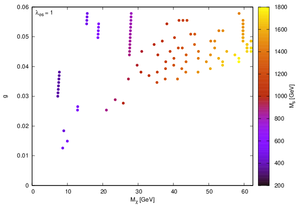
In Fig. 14, ranges of parameters space in mass of fermionic DM and coupling which are consistent with observed relic density have been shown. Comparing Figures 14 and 12-b shows that the allowed region for invisible Higgs decay and the DM relic density does not overlap with each other. Since the most contribution of DM relic density arises from fermionic DM, for small value of coupling, the annihilation of DM to SM particles will be suppressed. This means for portion of parameters space which is consistent with invisible Higgs decay, the relic density exceed the value of Planck measurement. Therefore, in order to evade invisible Higgs constraints, one should assume that fermionic DM mass is larger than .
6 Concluding remarks
Motivated by DM and hierarchy problems, we presented a scale-invariant extension of SM. In order to have a scale invariant version of the SM with scalar DM, at least two more scalars must be added to the theory. Moreover, in the absence of additional fermionic fields, the model has a small number of independent parameters which complicates the satisfying all theoretical and phenomenological constraints. Given these conditions, we added a scalon field , a scalar field and a fermionic field as two-component DM to SM. To summarize, the main novelty of this model with respect to other two-component DM models, is a much lower number of independent parameters due to scale invariant conditions.
In this analysis, relic density of two component DM was computed. We have shown that the most part of contribution of DM relic density arises from fermionic DM. We have discussed the allowed regions in parameter space of our model consistent with the observed relic density.
We have also taken into account the constraints of indirect detection and direct detection of DM. In order to constrain the parameter space of our model, we also checked the limits from self interaction of DM. It is shown that the former analysis can not put constraint on the model in large portion of parameters space. Only in the vicinity of the resonances in for scalar DM and or for fermionic DM, self-interaction scenario constraints the model.
Finally, we probed the limits from the invisible decay width of the Higgs. We have found that the viable regions in parameter space are in agreement with upper limit on the invisible Higgs decay branching ratio. We compared the consistent region in parameter space for invisible Higgs decay with the relic density of the fermionic DM and show that in order to satisfy invisible Higgs constraints, fermionic DM mass should be larger than .
Acknowledgement
The authors would like to thank S. Paktinat for careful reading of the manuscript and the useful remarks.
Appendix: DM self-interaction cross sections and Decay Rates
In this appendix, we summarize the formula of the self-interacting cross-sections for two components of DM and decay rates of two scalars Higgs.
The main contribution to for scalar annihilation (processes [16], and ) in the non-relativistic limit are given by:
| (47) |
| (48) |
where is the usual Mandelstem variable and the decay rate for and are expressed by:
| (49) | ||||
| (50) |
In the following, we calculate self-interaction for the case of Dirac fermionic DM which includes processes and . The cross section of these processes are given by:
| (51) |
| (52) |
We also calculate the DM self scattering cross-sections for processes in non-relativistic limit. The cross sections can be written as:
| (53) |
where , and are momentum of initial fermionic DM, energy of initial fermionic DM and energy of final fermionic DM, respectively.
We also calculate the following formula for decay rates of , and :
| (54) | ||||
| (55) | ||||
| (56) |
where
References
- [1] A. M. Sirunyan et al. [CMS Collaboration], JHEP 1712 (2017) 142 doi:10.1007/JHEP12(2017)142 [arXiv:1707.06193 [hep-ex]]; C. Autermann [ATLAS and CMS Collaborations], EPJ Web Conf. 164 (2017) 01028. doi:10.1051/epjconf/201716401028; CMS Collaboration [CMS Collaboration], CMS-PAS-SUS-17-012; M. Aaboud et al. [ATLAS Collaboration], Phys. Rev. D 98 (2018) no.3, 032009 doi:10.1103/PhysRevD.98.032009 [arXiv:1804.03602 [hep-ex]]; M. Aaboud et al. [ATLAS Collaboration], Phys. Rev. D 97 (2018) no.9, 092006 doi:10.1103/PhysRevD.97.092006 [arXiv:1802.03158 [hep-ex]]; M. Aaboud et al. [ATLAS Collaboration], JHEP 1806 (2018) 107 doi:10.1007/JHEP06(2018)107 [arXiv:1711.01901 [hep-ex]].
- [2] E. Gildener and S. Weinberg, Phys. Rev. D 13 (1976) 3333. doi:10.1103/PhysRevD.13.3333
- [3] S.R. Coleman and E.J. , Phys. Rev. D 7 (1973) 1888.
- [4] K.A. Meissner and H. Nicolai, , Phys. Lett. B 648 (2007) 312 [hep-th/0612165]; R. Foot, A. Kobakhidze, K.L. McDonald and R.R. Volkas, Phys. Rev. D 77 (2008) 035006 [arXiv:0709.2750]; C. Cosme, J. G. Rosa and O. Bertolami, JHEP 1805 (2018) 129 doi:10.1007/JHEP05(2018)129 [arXiv:1802.09434 [hep-ph]]; K. Kannike, M. Raidal, C. Spethmann and H. Veermäe, JHEP 1704 (2017) 026 doi:10.1007/JHEP04(2017)026 [arXiv:1610.06571 [hep-ph]]; A. Karam and K. Tamvakis, Phys. Rev. D 94 (2016) no.5, 055004 doi:10.1103/PhysRevD.94.055004 [arXiv:1607.01001 [hep-ph]]; V. V. Khoze and A. D. Plascencia, JHEP 1611 (2016) 025 doi:10.1007/JHEP11(2016)025 [arXiv:1605.06834 [hep-ph]]; A. Ahriche, A. Manning, K. L. McDonald and S. Nasri, Phys. Rev. D 94 (2016) no.5, 053005 doi:10.1103/PhysRevD.94.053005 [arXiv:1604.05995 [hep-ph]]; A. Karam and K. Tamvakis, Phys. Rev. D 92 (2015) no.7, 075010 doi:10.1103/PhysRevD.92.075010 [arXiv:1508.03031 [hep-ph]]; S. Benic and B. Radovcic, JHEP 1501 (2015) 143 doi:10.1007/JHEP01(2015)143 [arXiv:1409.5776 [hep-ph]].
- [5] J. H. Huh, J. E. Kim and B. Kyae, Phys. Rev. D 79, 063529 (2009) doi:10.1103/PhysRevD.79.063529 [arXiv:0809.2601 [hep-ph]]; S. Bhattacharya, A. Drozd, B. Grzadkowski and J. Wudka, JHEP 1310, 158 (2013) doi:10.1007/JHEP10(2013)158 [arXiv:1309.2986 [hep-ph]]; A. Biswas, D. Majumdar and P. Roy, JHEP 1504, 065 (2015) doi:10.1007/JHEP04(2015)065 [arXiv:1501.02666 [hep-ph]]; A. Biswas, D. Majumdar, A. Sil and P. Bhattacharjee, JCAP 1312, 049 (2013) doi:10.1088/1475-7516/2013/12/049 [arXiv:1301.3668 [hep-ph]]; S. Esch, M. Klasen and C. E. Yaguna, JHEP 1409, 108 (2014) doi:10.1007/JHEP09(2014)108 [arXiv:1406.0617 [hep-ph]]; A. Biswas, J. Phys. G 43, no. 5, 055201 (2016) doi:10.1088/0954-3899/43/5/055201 [arXiv:1412.1663 [hep-ph]]; L. Bian, R. Ding and B. Zhu, Phys. Lett. B 728, 105 (2014) doi:10.1016/j.physletb.2013.11.034 [arXiv:1308.3851 [hep-ph]]; Y. Daikoku, H. Okada and T. Toma, Prog. Theor. Phys. 126, 855 (2011) doi:10.1143/PTP.126.855 [arXiv:1106.4717 [hep-ph]]; L. Bian, T. Li, J. Shu and X. C. Wang, JHEP 1503, 126 (2015) doi:10.1007/JHEP03(2015)126 [arXiv:1412.5443 [hep-ph]]; A. Dutta Banik, M. Pandey, D. Majumdar and A. Biswas, Eur. Phys. J. C 77, no. 10, 657 (2017) doi:10.1140/epjc/s10052-017-5221-y [arXiv:1612.08621 [hep-ph]]; K. Belotsky, M. Khlopov, C. Kouvaris and M. Laletin, Int. J. Mod. Phys. D 24, no. 13, 1545004 (2015) doi:10.1142/S0218271815450042 [arXiv:1508.02881 [astro-ph.HE]]; M. Aoki and T. Toma, JCAP 1701, no. 01, 042 (2017) doi:10.1088/1475-7516/2017/01/042 [arXiv:1611.06746 [hep-ph]]; M. Pandey, D. Majumdar and K. P. Modak, JCAP 1806, no. 06, 023 (2018) doi:10.1088/1475-7516/2018/06/023 [arXiv:1709.05955 [hep-ph]]; S. Peyman Zakeri, S. Mohammad Moosavi Nejad, M. Zakeri and S. Yaser Ayazi, Chin. Phys. C 42, no. 7, 073101 (2018) doi:10.1088/1674-1137/42/7/073101 [arXiv:1801.09115 [hep-ph]].
- [6] K. Ghorbani and H. Ghorbani, JHEP 1604 (2016) 024 doi:10.1007/JHEP04(2016)024 [arXiv:1511.08432 [hep-ph]].
- [7] G. Belanger, F. Boudjema, A. Pukhov and A. Semenov, Comput. Phys. Commun. 192, 322 (2015) doi:10.1016/j.cpc.2015.03.003 [arXiv:1407.6129 [hep-ph]].
- [8] A. Semenov, Comput. Phys. Commun. 180, 431 (2009) doi:10.1016/j.cpc.2008.10.012 [arXiv:0805.0555 [hep-ph]].
- [9] , P. A. R. Ade et al (Planck Collaboration), Astron. Astrophys, 571: A31 (2014)
- [10] E. Aprile et al. [XENON100 Collaboration], Phys. Rev. D 94 (2016) no.12, 122001 doi:10.1103/PhysRevD.94.122001 [arXiv:1609.06154 [astro-ph.CO]].
- [11] D. S. Akerib et al. [LUX Collaboration], Phys. Rev. Lett. 118 (2017) no.2, 021303 doi:10.1103/PhysRevLett.118.021303 [arXiv:1608.07648 [astro-ph.CO]].
- [12] X. G. He, T. Li, X. Q. Li, J. Tandean and H. C. Tsai, Phys. Rev. D 79 (2009) 023521 doi:10.1103/PhysRevD.79.023521 [arXiv:0811.0658 [hep-ph]].
- [13] G. Steigman, B. Dasgupta and J. F. Beacom, Phys. Rev. D 86 (2012) 023506 doi:10.1103/PhysRevD.86.023506 [arXiv:1204.3622 [hep-ph]].
- [14] F. Kahlhoefer, K. Schmidt-Hoberg, J. Kummer and S. Sarkar, Mon. Not. Roy. Astron. Soc. 452 (2015) no.1, L54 doi:10.1093/mnrasl/slv088 [arXiv:1504.06576 [astro-ph.CO]].
- [15] M. Kaplinghat, S. Tulin and H. B. Yu, Phys. Rev. Lett. 116 (2016) no.4, 041302 doi:10.1103/PhysRevLett.116.041302 [arXiv:1508.03339 [astro-ph.CO]].
- [16] R. Campbell, S. Godfrey, H. E. Logan, A. D. Peterson and A. Poulin, Phys. Rev. D 92 (2015) no.5, 055031.
- [17] S. Dittmaier et al. [LHC Higgs Cross Section Working Group], doi:10.5170/CERN-2011-002 arXiv:1101.0593 [hep-ph].
- [18] CMS Collaboration [CMS Collaboration], CMS-PAS-HIG-14-038.
- [19] The ATLAS collaboration [ATLAS Collaboration], ATLAS-CONF-2015-004.
- [20] G. Belanger, B. Dumont, U. Ellwanger, J. F. Gunion and S. Kraml, Phys. Lett. B 723 (2013) 340 doi:10.1016/j.physletb.2013.05.024 [arXiv:1302.5694 [hep-ph]].
- [21] S. Heinemeyer et al. [LHC Higgs Cross Section Working Group], doi:10.5170/CERN-2013-004 arXiv:1307.1347 [hep-ph].