Regression adjustments for estimating the global treatment effect in experiments with interference Thanks: The author thanks Fredrik Sävje, Johan Ugander, and seminar participants at Facebook, Stanford University, and Yale University for helpful comments and suggestions. This work was supported in part by NSF grant IIS-1657104.
Abstract
Standard estimators of the global average treatment effect can be biased in the presence of interference. This paper proposes regression adjustment estimators for removing bias due to interference in Bernoulli randomized experiments. We use a fitted model to predict the counterfactual outcomes of global control and global treatment. Our work differs from standard regression adjustments in that the adjustment variables are constructed from functions of the treatment assignment vector, and that we allow the researcher to use a collection of any functions correlated with the response, turning the problem of detecting interference into a feature engineering problem. We characterize the distribution of the proposed estimator in a linear model setting and connect the results to the standard theory of regression adjustments under SUTVA. We then propose an estimator that allows for flexible machine learning estimators to be used for fitting a nonlinear interference functional form. We propose conducting statistical inference via bootstrap and resampling methods, which allow us to sidestep the complicated dependences implied by interference and instead rely on empirical covariance structures. Such variance estimation relies on an exogeneity assumption akin to the standard unconfoundedness assumption invoked in observational studies. In simulation experiments, our methods are better at debiasing estimates than existing inverse propensity weighted estimators based on neighborhood exposure modeling. We use our method to reanalyze an experiment concerning weather insurance adoption conducted on a collection of villages in rural China.
Keywords: causal inference, peer effects, SUTVA, A/B testing, exposure models, off-policy evaluation
1 Introduction
The goal in a randomized experiment is often to estimate the total or global average treatment effect (GATE) of a binary treatment variable on a response variable. The GATE is the difference in average outcomes when all units are exposed to treatment versus when all units are exposed to control. Under the standard assumption that units do not interfere with each other [Cox 1958], which forms a key part of the stable unit treatment value assumption (SUTVA) [Rubin 1974, Rubin 1980], the global average treatment effect reduces to the standard average treatment effect.
However, in many social, medical, and online settings the no-interference assumption may fail to hold [Rosenbaum 2007, Walker and Muchnik 2014, Aral 2016, Taylor and Eckles 2017]. In such settings, peer and spillover effects can bias estimates of the global average treatment effect. In the past decade, there has been a flurry of literature proposing methods for handling interference, mostly focusing on cases in which structural assumptions about the nature of interference are known. For example, if there is a natural grouping structure to the data, such as households or schools or classrooms, it may be reasonable to assume that interference exists within but not across groups. Versions of this assumption are known as partial or stratified interference [Hudgens and Halloran 2008]. In this case two-stage randomized designs can be used to decompose direct and indirect effects, which is an approach studied by VanderWeele and Tchetgen Tchetgen [2011], Tchetgen Tchetgen and VanderWeele [2012], Liu and Hudgens [2014], Baird et al. [2016], Basse et al. [2017], among others. Baird et al. [2016] study how two-stage, random saturation designs can be used to estimate dose response curves under the stratified interference assumption. Basse and Feller [2018] study two-stage experiments in which households with multiple students are assigned to treatment or control. Other works that propose methods of handling interference include Ogburn and VanderWeele [2014], which maps out causal diagrams for interference; van der Laan [2014], which studies a targeted maximum likelihood estimator for the case where network connections and treatments possibly change over time; Choi [2017], which shows how confidence intervals can be constructed in the presence of monotone treatment effects; and Jagadeesan et al. [2017], which studies designs for estimating the direct effect that strive to balance the network degrees of treated and control units.
The modus operandi for general or arbitrary interference is the method of exposure modeling, in which the researcher defines equivalence classes of treatments that inform the interference pattern. Aronow and Samii [2017] develop a general framework for analyzing inverse propensity weighted (Horvitz-Thompson- and Hájek-style) estimators under correct specification of local exposure models. The exposure model often used is some version of an assumption that the potential outcomes of unit are constant conditional on all treatments in a local neighborhood of , or that the potential outcomes are a monotone function of such treatments. This assumption, known as neighborhood treatment response (NTR), is a generalization of partial and stratified interference to the general network setting [Manski 2013]. Methods for handling interference often rely on neighborhood treatment response as a core assumption. For example, Sussman and Airoldi [2017] develop unbiased estimators for various parametric models of interference that are all restrictions on the NTR condition, and Forastiere et al. [2016] propose propensity score estimators for observational studies using the NTR assumption.
Aronow and Samii [2017] use their methods to analyze the results of a field experiment on an anti-conflict program in middle schools in New Jersey. By defining appropriate exposure models, they are able to estimate a direct effect (the effect of receiving the anti-conflict intervention), a spillover effect (the effect of being friends with some students who received the anti-conflict intervention), and a school effect (the effect of attending a school in which some students received the anti-conflict intervention). The network structure consists of 56 disjoint social networks (schools), comprising 24,191 students in the original Paluck et al. [2016] study and a subset of 2,050 students studied in the Aronow and Samii [2017] analysis. There are a number of similar studies in which the target of scientific inquiry is the quantification of peer or spillover effects and where the dataset permits doing so by being comprised of “many sparse networks.” Studies which consist of randomized experiments on such social networks include Banerjee et al. [2013], which studies a microfinance loan program in villages in India; Cai et al. [2015], which studies a weather insurance program for farmers in rural China; Kim et al. [2015], which concerns public health interventions such as water purification and microvitamin tablets in villages in Honduras; and Beaman et al. [2018], which explores social diffusion of a new agricultural technology among farmers in Malawi. (Some studies thereof do not explicitly aim to understand spillover effects—for example Kim et al. [2015] and Beaman et al. [2018] are concerned primarily with strategies for targeting influential individuals—but the presence of such effects is still crucial for their purposes.) In these settings, exposure modeling may be (and has been) a successful way of decomposing direct and spillover effects.
The difficulties of using exposure models for global effects
How should one proceed if the goal is estimation of the global treatment effect rather than a decomposition into direct and spillover effects? In this setting interference is a nuisance, not an object of intrinsic scientific interest. Unbiased estimation would result from using an exposure model that accurately represents the true data-generating process. However, the complicated nature of social interactions makes it difficult to select an exposure model that is both tractable and well-specified. Eckles et al. [2017] discuss some of the difficulties of working in this setting in the context of “implausibility of tractable treatment response assumptions”:
It is unclear how substantive judgment can directly inform the selection of an exposure model for interference in networks—at least when the vast majority of vertices are in a single connected component. Interference is often expected because of social interactions (i.e., peer effects) where vertices respond to their neighbors’ behaviors: in discrete time, the behavior of a vertex at is affected by the behavior of its neighbors at ; if this is the case, then the behavior of a vertex at would also be affected by the behavior of its neighbors’ neighbors at , and so forth. Such a process will result in violations of the NTR assumption, and many other assumptions that would make analysis tractable.
In this setting, one primary tool that has developed in the literature is the method of graph cluster randomization [Ugander et al. 2013], where researchers use a clustered design in which the clusters are selected according to the structure of the graph in order to lower the variance of NTR-based inverse propensity estimators. Eckles et al. [2017] provide theoretical results and simulation experiments to show how clustered designs can reduce bias due to interference. Clusters can be obtained using algorithms developed in the graph partitioning and community detection literature [Fortunato 2010, Ugander and Backstrom 2013].
While the graph clustering approach can be effective at removing some bias, the structure of real-world empirical networks may make it difficult to obtain satisfactory bias reduction via clustering, which relies on having good quality graph cuts. The “six degrees of separation” phenomenon is well-documented in large social networks [Ugander et al. 2011, Backstrom et al. 2012], and the average distance between two Facebook users in February 2016 was just 3.5 [Bhagat et al. 2016]. Furthermore, most users belong to one large connected component and are unlikely to separate cleanly into evenly-sized clusters. In a graph clustered experiment run at LinkedIn, the optimal clustering strategy used maintained only 35.59% of edges between nodes of the same cluster [Saveski et al. 2017, Table 1], suggesting that bias remains even after clustering. Figure 1 provides an example illustration of how the structure of the network can markedly affect how much we might expect cluster randomization to help.

Such experimental designs also face practical hurdles. Though cluster randomized controlled trials are commonly used in science and medicine, existing experimentation platform infrastructure in some organizations may only exist for standard (i.i.d.) randomized experiments, in which case adapting the design and analysis pipelines for graph cluster randomization would require significant ad hoc engineering effort. In regimes of only mild interference, it may simply not be worth the trouble to run a clustered or two-stage experiment, especially if there is no way to know a priori how much bias from interference will be present. Instead, the practitioner would prefer to have a data-adaptive debiasing mechanism that can be applied to an experiment that has already been run. Ideally, such estimators provide robustness to deviations from SUTVA yet do not sacrifice too much in precision loss if it turns out interference was weak or non-existent.
Towards an agnostic regression approach
We can take advantage of the fact that the global treatment effect estimand, as opposed to a peer or spillover effect estimand, can be defined agnostically without regard to any exposure model. The exposure model used, therefore, matters only insofar as it informs the corresponding estimator used. An appropriate exposure model is one that leads to estimates of the global treatment effect that are approximately unbiased, even if it is not the exposure model corresponding to the true data-generating process. This agnostic perspective gives us hope because of the decoupling between data generation and estimation: We can believe in a complex interference pattern without having to use the corresponding intractable exposure model for estimation.
Our approach is motivated by the rich literature on regression adjustment estimators in the non-interference setting. In randomized controlled trials, regression adjustments are used to adjust for imbalances due to randomized assignment of the empirical covariate distributions of different treatment groups, and thus improve precision of treatment effect estimators. In the observational studies setting, regression adjustments are used to adjust for inherent differences between the covariate distributions of different treatment groups. We heavily borrow tools from that literature, both in the classical regime of using low-dimensional, linear regression estimators [Freedman 2008a, Freedman 2008b, Lin 2013, Berk et al. 2013] and more recent advancements that can utilize high-dimensional regression and machine learning techniques [Bloniarz et al. 2016, Wager et al. 2016, Wu and Gagnon-Bartsch 2017, Athey et al. 2017b, Chernozhukov et al. 2018]. This recent literature adopts the agnostic perspective that properties of least squares and machine learning estimators can be utilized without assuming the parametric model itself.
This paper contains two main contributions: (a) a regression adjustment strategy for debiasing global treatment effect estimators, and (b) a class of bootstrapping and resampling methods for constructing variance estimates of such estimators. We explore how well the analysis side of an experiment can be improved in independently-assigned (non-clustered) experiments. Our approach can be loosely motivated by the linear-in-means (LIM) family of models from the econometrics literature [Manski 1993]. In a simple version of this model, an individual’s outcome is said to depend on the average of her peer’s exogenous features. If this is true, then the peer average feature “statistic” can be adjusted for when estimating the global treatment effect, even if the linear-in-means model itself does not hold. We note that much of the linear-in-means literature focuses on the identifiability of various peer effect parameters within the LIM model [Bramoullé et al. 2009]; our goal instead is estimation of the agnostic global effect.
Generally, our strategy is to learn a statistical model that captures the relationship between the outcomes and a set of unit-level statistics constructed from the treatment vector and the observed network. These statistics can be viewed as features or adjustment variables, and are to be constructed by the practitioner using domain knowledge. The model is then used to predict the unobserved potential outcomes of each unit under the counterfactual scenarios if the unit had been assigned to global treatment, and global control. The approach is thus reminiscent of regression adjustment estimators and off-policy evaluation. Figure 2 demonstrates how feature distributions differ between the observed design distribution and the unobserved global counterfactual distributions of interest.
In Section 3 we present estimators in the context of a generative linear model and in Section 4 we discuss the non-linear analog. Even though the results in this paper are presented within the context of a generative model, they still make progress towards a fully agnostic solution. First, the models considered here are considerably more flexible, and more easily extended, than exposure models (which are also assumed to be generative). Second, the assumptions on the errors can be relaxed and we show via simulation experiments (Section 5) that these linear methods can work well in more general contexts. The non-linear context, which allows the use of arbitrary machine learning estimators, also moves closer to a fully agnostic approach by allowing a nonparametric generative model. Third, by connecting these results to analogous ones in the SUTVA case we lay the foundation for how to think about an agnostic approach, which is not possible using pure exposure modeling methods. Indeed, agnostic perspectives have emerged only recently even in the SUTVA setting [Freedman 2008a, Freedman 2008b, Lin 2013]. This paper, therefore, can be viewed as a conceptual stepping stone between existing methods that assume exposure models are generative, and future work that would establish a fully agnostic presentation.

It is shown in this paper that an assumption of exogeneity is required, even though the treatment is randomized. Such an assumption can be likened to an unconfoundedness, ignorability, or selection on observables assumption. A curious feature of randomized experiments under interference, then, is that they display characteristics of observational studies as well. It is helpful to think of estimators used in SUTVA observational studies that require the estimation of both a propensity model and a response model. (Doubly-robust estimators allow misspecification of one but not both of these models.) In a randomized experiment under interference the propensity model is fully known and does not need to be estimated; however, the response can be affected by confounding variables. In randomized experiments under interference, then, researchers must be wary of the same challenges that beset drawing causal conclusions from observational datasets, even though the treatments were assigned randomly. The exogeneity assumption is not generally verifiable from the data but is necessary in order to make any progress. Ideally, one has access to methods for conducting sensitivity analyses for interference, but such methods are in their infancy and we refrain from addressing this issue here.
Our estimators have several advantages over existing exposure modeling estimators. The correct specification of an exposure model is also a form of exogeneity assumption, yet our approach admits much more flexible forms of interference. It can handle multiple types of graph features, which do not even have to be constructed from the same network. Adjusting for interference becomes a feature engineering problem in which the practitioner is free to use his or her domain knowledge to construct appropriate features. If a feature turns out to be noninformative for interference, no additional bias is incurred (though a penalty in variance may be paid). Our adjustment framework also reduces to the standard, SUTVA regression adjustment setup in the event that static, baseline characteristics are used.
Finally, we propose methods for quantifying the variance of the proposed estimators. Variance estimation in the presence of interference is generally difficult because of the complicated dependencies created by the propagation of interference over the network structure. Confidence intervals based on asymptotic approximations may not be reliable since the dependencies can drastically reduce the effective sample size. For example, the variance of the sample mean of the features may not even scale at a rate, where is the sample size. In this paper we propose a novel way of taking advantage of the randomization distribution to produce bootstrap standard errors, assuming unconfoundedness. Since the features are constructed by the researcher from the vector of treatments, and the distribution of treatments is known completely in a randomized experiment, we can calculate via Monte Carlo simulation the sampling distribution of any function of the design matrix under the randomization distribution. This approach ensures that we properly represent all of the dependencies exhibited empirically by the data, and can then be used to construct standard errors.
The remainder of this paper is structured as follows. In Section 2 we describe the problem and motivate our approach with an informal discussion of a linear-in-means model. In Section 3 we develop the main results for linear regression estimators and in Section 4 we show how to extend this to the non-linear setting. In Section 5 we conduct simulation experiments, in Section 6 we consider an application to an existing field experiment, and in Section 7 we conclude. All proofs are in the appendix.
2 Setup and estimation in LIM models
We work within the potential outcomes framework, or Rubin causal model [Neyman 1923, Rubin 1974]. Consider a population of units indexed on the set and let be a random vector of binary treatments. We will work only with treatments assigned according to a Bernoulli randomized experimental design:
Assumption 1.
for every unit , where is the treatment assignment probability.
The general spirit of our approach can likely be extended to more complicated designs, but our goal in this paper is to show that substantial analysis-side improvements can be made even under the simplest possible experimental design.
Suppose that each response lives in an outcome space , and is determined by a mean function :
| (1) |
In this section we limit ourselves to an informal discussion of point estimation and defer the question of variance estimation to a future section. The only assumption we require on the residuals, therefore, is an assumption of strict exogeneity:
In particular, no independence or other assumptions about the correlational structure of the residuals are made in this section, though such assumptions will be necessary for variance estimation, which we address in Section 3.
Because the units are assumed to belong to a network structure, distinguishing between finite population and infinite superpopulation setups is not so straightforward. In the SUTVA setting, good estimators for finite population estimands (or conditional average treatment effects) are usually good estimators for superpopulation estimands, and vice versa [Imbens 2004]. In order to simplify the analysis, we do not work with a fixed potential outcomes for , and allow the residuals to be random variables. We therefore consider additional variation of the potential outcomes coming from repetitions of the experiment, but we do not consider the units to be sampled from a larger population. We do this because it is easier to discuss the behavior of when they are random variables. This perspective is related to the intrinsic nondeterminism perspective discussed by Pearl [2009] on page 220, as well as the idea of stochastic counterfactuals discussed previously in the literature [Greenland 1987, Robins and Greenland 1989, Robins and Greenland 2000, VanderWeele and Robins 2012].
In this paper we focus on estimation of the total or global average treatment effect (GATE), defined by
| (2) |
This parameter is called a global treatment effect because is a contrast of average outcomes between the cases when the units are globally exposed to treatment () and globally exposed to control ().
Under an assumption of strict exogeneity, in which , the treatment effect is the difference of average global exposure means
In order to proceed, we must make assumptions about the structure of the mean function .
2.1 A simple linear-in-means model
To illustrate our approach we start with a simple model. Let be a network with adjacency matrix . For simplicity in this paper we will mostly assume that is simple and undirected, but one can just as easily use a weighted and directed graph. We emphasize that we assume is completely known to the researcher. Let be the neighborhood of unit and be the network degree of unit . Define
| (3) |
the fraction of neighbors of that are in the treatment group. Then take the mean function in equation (1) to be as follows.
Model 1 (Exogenous LIM model).
This model is a simple version of a linear-in-means model [Manski 1993]. The model contains an intercept as well as a direct effect , which captures the strength of individual ’s response to changes in its own treatment assignment. Additionally, the response of unit is correlated with mean treatment assignment of its neighbors; Manski [1993] calls an exogenous social effect, because it captures the correlation of unit ’s response with the exogenous characteristics of its neighbors. The interactions are also assumed to be “anonymous” in that the unit responds only to the mean neighborhood treatment assignment and not the identities of those treated neighbors. In this model, unit responds to its neighbors’ treatments but not to its neighbors’ outcomes. Under Model 1, the variable is the mechanism by which interference affects the outcome and thus can be viewed as playing a similar role as baseline characteristics or pretreatment covariates in an observational study. However, in this paper we shall use the term statistic or feature rather than covariate to refer to , in order to remind the reader that does not represent a baseline characteristic.
Now consider the estimand (2) under Model 1. If all units are globally exposed to treatment then it is the case for all units that and . Therefore
Similarly, if all units are globally exposed to control, then and , and so
Therefore, the treatment effect under Model 1 is simply
This parametrization suggests that if we have access to unbiased estimators and for and , then an unbiased estimate for is given by
In particular, one is tempted to estimate and with an OLS regression of on and . Of course, using as an estimator for only makes sense if Model 1 accurately represents the true data generating process. We build up more flexible models in the following sections.
In contrast, we can easily see why the difference-in-means estimator, defined for sample sizes and as
| (4) |
is biased under Model 1. The mean treated response is
where is independent of since the treatments are assigned independently and there are no self-loops in . Similarly,
Therefore, the difference-in-means estimator has expectation , which need not equal in general. Only if do they coincide, in which case SUTVA holds and there is no interference. In other words, the difference-in-means estimator marginalizes out the indirect effect rather than adjusting for it; it is an unbiased estimator not for the GATE but for the expected average treatment effect (EATE), defined as
The EATE was introduced in Sävje et al. [2017] as a natural object of study for estimators which are designed for the SUTVA setting. Sävje et al. [2017], Chin [2018] study the limiting behavior of estimators such as under mild regimes of misspecification of SUTVA due to interference.
2.2 Linear-in-means with endogenous effects
Now we move to the more interesting version of the linear-in-means model, which contains an endogenous social effect in addition to an exogenous one. Let
| (5) |
the average value of the neighboring responses. Now consider the following model:
Model 2(a) (LIM with endogenous social effect).
In addition to direct and exogenous spillover effects, unit now depends on the outcomes of its neighbors through the spillover effect . It is conventional and reasonable to assume that . Model 2(a) is often more realistic than Model 1; as discussed in the introduction, we often believe that interference is caused by individuals reacting to their peers’ behaviors rather than to their peers’ treatment assignments.
It is helpful to write Model 2(a) in vector-matrix form. Let be the weighted graph defined by degree-normalizing the adjacency matrix of ; i.e., let be the graph corresponding to the adjacency matrix with entries . Then the matrix representation of Model 2(a) is
| (6) |
where , , and are the -vectors of responses, treatment assignments, and residuals, respectively. Using the matrix identity , as in equation (6) of Bramoullé et al. [2009], one obtains the reduced form
Unlike Manski [1993], Bramoullé et al. [2009] and other works in the “reflection problem” literature, we are not concerned with the identification of the social effect parameters and ; these are only nuisance parameters toward the end of estimating . We do note, however, that conditions for identifiability are generally mild enough to be satisfied by real-world networks. For example, Bramoullé et al. [2009] show that the parameters in Model 2(a) are identified whenever there exist a triple of individuals who are not all pairwise friends with each other; such a triple nearly certainly exists in any networks that we consider.
Now, let be the -th coordinate of . That is,
and in general, for any ,
Then Model 2(a) is the same as
| (7) |
where we have reparametrized the coefficients as
Notice that equation (7) respects exogeneity, as
Each feature represents the effect of treatments from units of graph distance on the response of unit . Since , the effects of the terms do not contribute much to equation (7) when is large. Therefore, for any finite integer , we may consider approximating Model 2(a) with a finite-dimensional model.
Model 2(b) (Finite linear-in-means).
| (8) |
The approximation error is of order (recall that ). Therefore, good estimates of the coefficients in equation (8) should be good estimates of the coefficients in equation (7) as well. Unless spillover effects are extremely large, the approximation may be quite good for even small values of . In fact, it may be reasonable to take equation (8) rather than equation (7) as the truth where is no larger than the diameter of the network , as spillovers for larger distances may not make sense.
As in Model 1, we can consider the counterfactuals of interest. If all units are globally exposed to treatment, then and for all and . Similarly, if all units are globally exposed to control, then and for all and . Therefore, by equation (7), the estimand under Model 2(a) is
and under Model 2(b) it is
Now, since Model 2(b) has only coefficients, given individuals one can estimate the coefficients using, say, ordinary least squares. The treatment effect estimator
is then unbiased for under Model 2(b) and “approximately unbiased” for under Model 2(a). This discussion is of course quite informal, and we make more formal arguments in Section 3.
One interpretation of the discussion in this section is that an endogeneous social effect in the linear-in-means model manifests as a propogation of exogenous effects through the social network, with the strength of the exogenous effect diminishing as the network distance increases. Therefore, adjusting for the exogenous features within the first few neighborhoods is nearly equivalent to adjusting for the behavior implied by the endogenous social effect.
2.3 Model assumptions and exposure models
The statements of the models discussed in this section couple together an interference mechanism restriction with a functional form assumption. It is worth disentangling these assumptions and discussing why it may be sometimes advantageous for the analyst to consider them jointly. First consider Model 1. It implies that the interference mechanism is restricted to influence from units only one step away in the graph, and furthermore, that this one-step influence is transmitted only through the statistic . This interference mechanism restriction can be framed in the language of constant treatment response (CTR) mappings [Manski 2013]:
| (9) |
The CTR statement (9) is equivalent to specifying an exposure model that the potential outcomes depend only on through and . However, it makes no assumptions about the functional form of , yet Model 1 goes further and makes a strong parametric functional form assumption about the response. It is conceptually useful to recognize the different meanings and implications of these assumptions.
One tempting approach, then, might be for an analyst to first consider verifying whether the exposure model holds, using domain knowledge or otherwise. The analyst then separately proceeds to consider appropriate functional forms (and perhaps only if nonparametric estimators exhibit low power). This logic may succeed for simple exposures of the form implied by Model 1 but can lead to issues for more complex data-generating processes likely to be encountered in the real world.
This is made clear by the discussion of Models 2(a) and 2(b). By rewriting Model 2(a) as the infinite series given by equation (7), we find that there is no data-reducing exposure model or CTR assumption that can handle such endogenous social effects! This is discouraging unless the analyst jointly considers the parametric implications of an endogenous effect , which suggests a way forward via the finite approximation Model 2(b). Even if the linearity in equation (8) is too strong, a natural relaxation might be a kind of generalized additive model of the form
where is arbitrary but is restricted to be decreasing in in order to ensure that spillovers decrease in graph distance.
Furthermore, statisticians are well-versed in distinguishing and handling modeling violations of the mean function (here, corresponding to the interference function form) and the covariance function (corresponding to the interference restriction assumption), whereas statements like (9) may be a bit more abstruse for the practicing statistician. The implications here are further clarified by the discussions in the following sections as well as the simulation examples provided in Section 5.
3 Interference features and the general linear model
In Section 2, we showed that the mean function in the linear-in-means model is comprised of a linear combination of statistics which are constructed as functions of the treatment vector. This fact suggests extending our approach to a linear model containing other functions of the treatment vector that are correlated with , not just the ones implied by the linear-in-means model. We now formulate the general linear model. We suppose that each unit is associated with a -dimensional vector of interference features or interference statistics that inform the pattern of interference for unit . We assume that the are low-dimensional (). Because is to be used for adjustment, the main requirement is that it not be a “post-treatment variable”; that is, that it not be correlated with the treatment . Therefore, we require the following assumption:
Assumption 2.
for all .
Let denote the vector of indirect treatments, which is the vector of all treatments except for . The key feature of our approach is that even though must be independent of , it is not necessary that be independent of the vector of indirect treatments . In fact, in order for to be useful for adjusting for interference, we expect that will be correlated with some entries of . In particular, may be a deterministic function of the indirect treatments,
| (10) |
Adjusting for such a variable will not cause post-treatment adjustment bias as long as the entries of are independent of each other. This holds automatically in a Bernoulli randomized design (Assumption 1).
The features may depend on static structural information about the units such as network information provided by , though since is static we supress this dependence in the notation. For example, defined as in equation (3), which represents the proportion of treated neighbors, captures a particular form of exogenous social influence. Provided there are no self-loops in so that , does not appear on the right-hand side of equation (3) and so and are independent.
We assume that we can easily sample from the distribution of . In particular, if , then the distribution of can be constructed by Monte Carlo sampling from the randomization distribution of the treatment . In this paper and in all the examples we use, we assume that is a function of as in equation (10), so that conditioning on removes all randomness in . But the generalization is easily handled.
In this section we assume that the response is linear in ; we address nonparametric response surfaces in Section 4.
Model 3 (Linear model).
Given , let the response follow
where the conditional response surfaces
satisfy
for and . That is, they follow a “separate slopes” linear model in . We assume .
In the above parametrization, we assume that the first coordinate of each is set to , so that the vectors and contain coefficients corresponding to the intercept as in the classical OLS formulation.
3.1 Feature engineering
Before considering assumptions on the residuals , we pause here to emphasize the flexibility provided by modeling the interference pattern as in Model 3. In this framework, the researcher can use domain knowledge to construct graph features that are expected to contribute to interference. In essence, we have transformed the problem of determining the structure of the interference pattern into a feature engineering problem, which is perhaps a more intuitive and accessible task for the practitioner.
To elaborate, consider the problem of selecting an exposure model. Ugander et al. [2013] propose and study a number of different exposure models for targeting the global treatment effect, including fractional exposure (based on the fraction of treated neighbors), absolute exposure (based on the raw number of treated neighbors), and extensions based on the -core structure of the network. In reality, it may be the case that fractional and absolute exposure both contribute partial effects of interference, so ideally one wishes to avoid having to choose between one of the two exposure models. On the other hand, both features are easily included in Model 3 by encoding both the fraction and raw number of treated neighbors in . (Including both features only makes sense when working with a complex network. If the interference structure is comprised of large, disjoint, and equally-sized clusters, as in partial interference, then the fraction and number of treated neighbors encode roughly the same information and one obtains a collinearity scenario that violates the full-rank assumption of Proposition 1. The methods in this paper are primarily motivated by the complex network setting.)
In a similar manner, the researcher may wish to handle longer-range interference, such as that coming from two-step or greater neighborhoods. It is possible to handle two-step information by working with the graph corresponding to the adjacency matrix , but this approach is unsatisfactory because presumably one-step interference is stronger than two-step interference, and this distinction is lost by using . On the other hand, if one-step and two-step network information are encoded as separate features, both effects are included and the magnitudes of their coefficients will reflect the strength of the corresponding interference contributed by each feature.
Furthermore, nothing in our framework requires the variables to be constructed from a single network. Often, the researcher has access to multiple networks defined on the same vertex set—i.e., a multilayer network [Kivelä et al. 2014]—representing different types of interactions among the units. For example, social networking sites such as Facebook and Twitter contain multiple friendship or follower networks based on the strength and type of interpersonal relationship (e.g. family, colleagues, and acquaintances), as well as activity-based networks constructed from event data such as posts, tweets, likes, or comments. Often these networks are also dynamic in time. Given the sociological phenomenon that the strength of a tie is an indicator of its capacity for social influence [Granovetter 1973] and that people use different mediums differently when communicating online [Haythornthwaite and Wellman 1998], any or all of these network layers can conceivably be a medium for interference in varying amounts depending on the treatment variable and outcome metric in question. In our framework graph features from different network layers are easily included in the model.
3.2 Exogeneity assumptions
Consider the following assumptions on the residuals.
Assumption 3.
- (a)
The errors are strictly exogenous: for all .
- (b)
The errors are independent.
- (c)
The errors are homoscedastic: for all .
Assumption 3(a) captures the requirement that the features contain all of the information needed to adjust for the bias contributed by interference, and thus is similar to an unconfoundedness or ignorability assumption often invoked in observational studies. Point estimates can be constructed based only on Assumption 3(a), but variance estimation requires Assumption 3(b) so that each data point contributes additional independent information. Note that in the SUTVA case Assumption 3(a) is all that is needed for valid inference. However under interference, it is possible that conditioning on the features removes all bias but interference is still present in the errors, in which case i.i.d.-based standard errors would be incorrect. These assumptions cannot be verified from the data, and so this setup borrows all of the problems that come with selecting an exposure model or being able to verify unconfoundedness. However, our setup is slightly different because of the flexibility afforded by the features. Compared to what we envision as the usual observational studies setting, our features are constructed from the treatment vector and social network rather than being collected in the wild, and so they are quite cheap to construct via feature engineering. That said, more work for conducting sensitivity analysis for interference or spillover effects is certainly needed.
Assumption 3(c) is the easiest to deal with if violated. One may use a heteroscedisticity-consistent estimate of the covariance matrix, also known as the sandwich estimator or the Eicker-Huber-White estimator [Eicker 1967, Huber 1967, White 1980]. In this paper we invoke Assumption 3(c) mainly to simplify notation, but heteroscedasticity-robust extensions are straightforward.
For following equation (10), denote
The variable represents the context for unit under the counterfactual scenario that is exposed to global control, and the variable represents the context for unit under the counterfactual scenario that exposed to global treatment. Both of these values are non-deterministic.11 1 In the event are not defined through a function , one may work with and , where this notation means that follows the conditional distribution of , conditionally on the event that , and similarly for . In this case and may be random, and estimands can be defined using and instead. For example, if be the “mean treated” statistic as defined in equation (3), then and for every unit .
We now consider the estimand under Model 3 and Assumption 3. The GATE for Model 3 is
where the second equality is by Assumption 3(a). Now introduce the quantities
which are the mean counterfactual feature values for global control and global treatment, averaged over the population. We emphasize that and are non-deterministic and known, because the distribution of is assumed to be known. We then have
| (11) |
Such an estimand, which focuses on the statistics of the finite population at hand, is natural in the network setting where there is no clear superpopulation or larger network of interest.
We now construct an estimator by estimating the regression coefficients with ordinary least squares. For , let be the design matrix corresponding to features belonging to treatment group , where the first column of is a column of ones. Let be the -vector of observed responses for treatment group . Then we use the standard OLS estimator
| (12) |
The estimate of the treatment effect is taken to be the difference in mean predicted outcomes under the global treatment and control counterfactual distributions,
| (13) |
Assuming Model 3 holds, is an unbiased estimate of , which follows from unbiasedness of the OLS coefficients.
Proposition 1.
Suppose Model 3 and Assumptions 1, 2, and 3(a) hold. Let and be defined as in equations (11) and (13), and let for be OLS estimators as defined in equation (12). Then conditionally on being full (column) rank,22 2 Since is random and depends on , conditioning on having full column rank is necessary, even though this condition may not be fulfilled for all realizations of the treatment vector. For example, if contains a column for the fraction of neighbors treated, then it is possible though highly unlikely for all units to be assigned to treatment, in which case this column is collinear with the intercept and is not full rank. We shall, for the most part, ignore this technicality and assume that the features are chosen so that the event that is singular doesn’t happen very often, and is in fact negligible asymptotically. Understanding combinations of network structures and interference mechanisms that give rise to singular is of interest to practitioners but outside the scope of our study here. is an unbiased estimator of and is an unbiased estimator of .
(Proofs for Proposition 1 and other results are deferred to the appendix.) Notice that the treatment group predicted mean is
and the control group predicted mean is
Therefore is linear in the observed response vector . That is, where the weight vectors and are given by
| (14) | ||||
| (15) |
These weights allow us to compare the reweighting strategy with that of other linear estimators, such as the Hájek estimator, which is a particular weighted mean of . More details are provided in Section 5.1, with an example given in Section 5.3.
3.3 Inference
Now we provide variance expressions under the assumption that the errors are exogenous, independent, and homoscedastic, as in Assumption 3.
Theorem 1.
3.3.1 Variance estimation
In order to estimate the variance (16), we must estimate the quantities and , which are the expected inverse sample covariance matrices. Of course, and are observed and unbiased estimators. However, unlike standard baseline characteristics collected in the wild, we envision that the are constructed from the graph and the treatment vector , and so we can take advantage of the fact that the distribution of is completely known to the researcher. It is thus possible to compute and up to arbitrary precision by repeated Monte Carlo sampling from the randomization distribution of . For clarity, this estimation procedure is illustrated in Algorithm 1.
Finally, we can estimate in the usual way, with the residual mean squared error
Equipped with and Monte Carlo estimates , we can use the variance estimate
| (17) |
3.4 Asymptotic results
Proposition 1 and Theorem 1 characterize the finite expectation and variance of the treatment effect estimator under Model 4. Establishing an asymptotic result is more nuanced, as because of the dependence among units implied by interference, the quantities and may not be in which case would not converge at a rate. This is a problem with dealing with interference in general, making comparisons to the semiparametric efficiency bound [Hahn 1998], a standard benchmark in the SUTVA case, difficult in this setting. However we can state a central limit theorem in the event that the sample mean and covariance do scale and converge appropriately. To do so, we implicitly assume existence of a sequence of populations indexed by their size , and that the parameters associated with each population setup, such as , , , and , converge to appropriate limits. Such an asymptotic regime is the standard for results of this sort [Freedman 2008a, Freedman 2008b, Lin 2013, Abadie et al. 2017a, Abadie et al. 2017b, Sävje et al. 2017, Chin 2018, cf.]. We suppress the index on to avoid notational clutter.
So that we can compare to previous works, it is helpful to reparametrize the linear regression setup so that the intercept and slope coefficients are written separately. That is, let and be redefined to exclude the intercept, and let so that the mean functions are written , where is the intercept parameter and is the vector of slope coefficients. Then the GATE is
Denote the within-group sample averages by
and
Since the intercept is determined by , the estimator , equation (13), is written as
| (18) |
Now, is seen to be an adjustment of the difference-in-means estimator . The adjustment depends on both the estimated strength of interference, , and the discrepancy between the means of the observed distribution and the reference or target distribution, . This linear shift is a motif in the regression adjustment literature, and is reminiscent of, e.g., equation (16) of Aronow and Middleton [2013].
We now state a central limit theorem for .
Theorem 2.
Assume the setup of Theorem 1. Assume further that the sample moments converge in probability:
where is positive definite, and that all fourth moments are bounded. Then , where
| (19) |
3.5 Relationship with standard regression adjustments
The practitioner may also wish to perform standard regression adjustments to adjust for static, contextual node-level variables such as age, gender, and other demographic variables. This fits easily into the framework of Model 4, as any such static variable can be viewed as simply a constant function of the indirect treatment vector . Then the adjustment is not used to remove bias but simply to reduce variance by balancing the feature distributions. In this case the counterfactual (global exposure) distribution is the same as the observed distribution, and in particular, and . Hence we see that Theorem 2 reduces to the standard asymptotic result for regression adjustments using OLS.
Corollary 1.
Assume the setup of Theorem 2. Suppose is independent of . Then and and
This variance in Corollary 1 is the same asymptotic variance as in the standard regression adjustment setup [cf. Wager et al. 2016, Theorem 2]. In practice, if some components of are static covariates and some are interference variables, then the resulting variance will be decomposed into the components stated in Theorem 2 and Corollary 1. Conditioning on both baseline covariates and interference features may in fact be necessary to ensure that Assumption 3(a) holds. For example if is the number of treated neighbors it may be believed that the potential outcomes depend on node degree (in the graph ) as well.
4 Nonparametric adjustments
In this section we relax the linear model, Model 3:
Model 4 (Non-linear response surface).
Let follow
with conditional mean response surfaces
We make no parametric assumptions on the form of and .
We maintain Assumption 3, namely that SUTVA holds conditionally on .
In the SUTVA setting, adjustment with OLS works best when the adjustment variables are highly correlated with the potential outcomes; that is, the precision improvement largely depends on the prediction accuracy. This fact suggests that predicted outcomes obtained from an arbitrary machine learning model can be used for adjustment, an idea formalized by Wager et al. [2016], Wu and Gagnon-Bartsch [2017]. Based on ideas from Aronow and Middleton [2013], these papers propose using the estimator
| (20) |
where and are predictions of the potential outcomes obtained without using the -th observation. This doubly-robust style approach is called cross-estimation by Wager et al. [2016] and the leave-one-out potential outcomes (LOOP) estimator by Wu and Gagnon-Bartsch [2017] who focus on imputing the outcomes using a version of leave-one-out cross validation. This estimator is also reminiscent of the double machine learning (DML) cross-fitting estimators developed for the observational study setting [Chernozhukov et al. 2018], which consists of the following two-stage procedure: (a) train predictive machine learning models of on (the propensity model) and of on (the response model), and then (b) use the out-of-sample residuals and in a final stage regression. The difference in the experimental setting is that the propensity scores are known and so no propensity model is needed. Wu and Gagnon-Bartsch [2017] study the behavior of (20) in the finite population setting where the only randomization comes from the treatment assignment, and Wager et al. [2016] provide asymptotic results for estimating the population average treatment effect. As long as the predicted value does not use the -th observation, estimator (20) allows us to obtain asymptotically unbiased adjustments and valid inference using machine learning algorithms such as random forests or neural networks. In practice, such predictions are obtained by a cross validation-style procedure in which the data are split into folds, and the predictions for each fold are obtained using a model fitted on data from the other folds. (Cross validation on graphs is in general difficult [Chen and Lei 2018, Li et al. 2018], but our procedure is unrelated to that problem because the features are constructed from the entire graph and fixed beforehand.)
In this section we apply insights from the above works to the interference setting. Under Model 4, the global average treatment effect has the form
To develop an estimator of , consider the form of the OLS estimator given by equation (18), which can be rewritten as
| (21) |
Now, by analog, we define the estimator for the nonparametric setting as
| (22) |
One sees that equations (21) and (22) agree whenever . Furthermore, equation (22) is equal to its SUTVA version, equation (20), whenever .
Because the units can be arbitrarily connected, the cross-fitting component partitions are not immediately guaranteed to be exactly independent, and so any theoretical guarantees must assume some form of approximate independence of the out-of-sample predictions. In this work we leave such theoretical results open for future work; our primary contribution is the proposal of estimator (22) and a bootstrap variance estimation method that respects the empirical structure of interference.
4.1 Bootstrap variance estimation
Here we discuss a method for placing error bars on the estimate defined in equation (22). We propose using a bootstrap estimator to estimate the sampling variance. Under exogeneity (Assumption 3), the features and residuals contribute orthogonally to the total variance, and so the model and residuals can be resampled separately.
Instead of using the fixed, observed as in a standard residual bootstrap, we propose capturing the entire variance induced by the feature distribution by sampling a new from its population distribution for each bootstrap replicate. That is, for each of bootstrap repetitions, we sample a new treatment vector and compute bootstrapped features . The means are then computed using the fitted function as and . Provided that the adjustments are consistent in the sup norm sense, that is, that
then , serve as appropriate stand-ins for , in large samples.
For the residual portion, we take the initial fitting functions and and compute the residuals
Under an assumption of independent errors, it is appropriate to compute bootstrap residuals by sampling with replacement from the observed residuals . We can then construct an artificial bootstrap response
We then compute using data , and then take the bootstrap distribution as an approximation to the true distribution of . To construct a confidence interval, one can calculate the endpoints using approximate Gaussian quantiles,
Alternatively, one may use the and quantiles of the empirical bootstrap distribution (a percentile bootstrap), which is preferable if the distribution of is skewed.
We wish to emphasize that the main insight here is that exogeneity allows the feature and residual variances to be handled separately, and that the feature variance can be computed from the design, however complicated the structure of itself may be. The bootstrap residuals as described above rely on independent errors, but in fact the practitioner is free to utilize the entirety of the rich bootstrap literature stemming from Efron [1979] in the event that this independence assumption is violated. For example, one may use versions of the block bootstrap [Künsch 1986] to try and protect against correlated errors. One can use more complicated bootstrap methods to be more faithful to the empirical distribution, such as incorporating higher-order features of the distribution via bias-corrected and accelerated (BCa) intervals [Efron 1987], or handling heteroscedasticity via the wild bootstrap [Wu 1986].
5 Simulations
This section is devoted to running a number of simulation experiments. Our goals in these simulations are to (a) verify that our adjustment estimators and variance estimates are behaving as intended, (b) compare the performance of our proposed estimators to that of existing inverse propensity weighted estimators based on exposure models, and (c) empirically explore the behavior of our estimators in regimes of mild model misspecification.
5.1 Simulation setup and review of exposure modeling
For the network we use a subset of empirical social networks from the facebook100 dataset, an assortment of complete online friendship networks for one hundred colleges and universities collected from a single-day snapshot of Facebook in September 2005. A detailed analysis of the social structure of these networks was given in Traud et al. [2011], Traud et al. [2012]. We use an empirical network rather than an instance of a random graph model in order to replicate as closely as possible the structural characteristics observed in real-world networks. We use the largest connected components of the Caltech and Stanford networks. Some summary statistics for the networks are given in Table 1.
| network | Caltech | Stanford |
|---|---|---|
| number of nodes | 762 | 11586 |
| number of edges | 16651 | 568309 |
| diameter | 6 | 9 |
| average pairwise distance | 2.33 | 2.82 |
In all simulation regimes we compare our regression estimators to two other estimators, which we describe now. As a baseline we use the SUTVA difference-in-means estimator
5.1.1 Exposure modeling IPW estimators
We also compare to an inverse propensity weighted estimator derived from a local neighborhood exposure model. We now briefly describe the exposure model-based estimators framed in the language of constant treatment response assumptions [Manski 2013]. For , this approach partitions the space of treatments into classes of treatments that map to the same mean response for unit . The partition function is assumed known, and is called an exposure function. The no-interference portion of SUTVA can be specified as an exposure model, since no-interference is equivalent to the requirement that for any two treatment vectors in which the -th components of and agree. Manski [2013] refers to this formulation as individualistic treatment response (ITR).
The exposure model most commonly used for local interference is the neighborhood treatment response (NTR) assumption, which given a graph , posits that whenever and agree in all components such that . In other words, NTR assumes that depends on unit ’s own treatment and possibly any other unit in its neighborhood , but that it does not respond to changes in the treatments of any units outside of its immediate neighborhood. For the purposes of estimating the global treatment effect, one may use fractional -NTR, where given a threshold parameter , -NTR assumes that a unit is effectively in global treatment if at least a fraction of its neighbors are assigned to treatment, and similarly for global control. NTR is thus a graph analog of partial interference for groups and -NTR is a corresponding version of stratified interference. The threshold is a tuning parameter; larger values of result in less bias due to interference, but greater variance because there are fewer units available for estimation. Eckles et al. [2017] provide some theoretical results for characterizing the amount of bias reduction. There is not much guidance for selecting to manage this bias-variance tradeoff; Eckles et al. [2017] uses .
Aronow and Samii [2017] study the behavior of inverse propensity weighted (IPW) estimators based on a well-specified exposure model. Toward this end, let
be the events that unit is -NTR exposed to global treatment and -NTR exposed to global control, respectively. Let their expectations be denoted by
which represent the propensity scores for unit being exposed to the global potential outcome conditions. Then the inverse propensity weighted estimators under consideration are defined as
| (23) |
The estimator is the Horvitz-Thompson estimator [Horvitz and Thompson 1952], and is the Hájek estimator [Hájek 1971]; these names stem from the survey sampling literature and are commonly used in the interference literature. In the importance sampling and off-policy evaluation literatures, analogs of and are known as unnormalized and self-normalized importance sampling estimators, respectively. In the finite potential outcomes framework The Horvitz-Thompson estimator is unbiased under the experimental design distribution, but suffers from excessive variance when the probabilities of global exposure are small, as is usually the case. The Hájek estimator, which forces the weights to sum to one and is thus interpretable as a difference of weighted within-group means, incurs a small amount of finite sample bias but is asymptotically unbiased, and is nearly always preferable to . For our simulations we will therefore avoid using .
One of the main insights in the exposure modeling framework developed by Aronow and Samii [2017] is that even if the initial treatment assignment probability is constant across units, the global treatment propensity scores need not be; indeed, and depend on the network structure and choice of exposure model. Therefore inverse propensity weighting is needed to produce unbiased (or consistent) estimators for contrasts between exposures even in a Bernoulli randomized design.
Given a design and a (simple enough) exposure model, the propensities can be calculated exactly. If the treatments are assigned according to independent Bernoulli coin flips, the exact exposure probabilities are expressed straightforwardly using the binomial distribution function. That is, for treatment probability and degree , the probability of unit being -NTR exposed to global treatment is
| (24) |
where
is the distribution function of a Binomial random variable. Similarly, the probability that unit is -NTR exposed to global control is
| (25) |
In a cluster randomized design, exposure probabilities for fractional neighborhood exposure can be computed using a dynamic program [Ugander et al. 2013].
A further comment on the propensity scores and is necessary. Importantly, these propensity scores are exact only to the extent to which the exposure model is correct. Thus, when the exposure model is unknown, these propensities scores should be viewed as estimated propensities, in which case even small estimation errors in the propensities can lead to large estimation errors in their inverses. It is therefore the case that and can suffer from the same high-variance problems as IPW estimators based on a fitted propensity model used in observational studies, even if the exposure model is only mildly misspecified.
In our simulations we use the Hájek estimator, , defined by equation (23) and the -NTR exposure probabilities (24) and (25). We fix , which is the same threshold used in Eckles et al. [2017]. For the other values of that we tried, performance was roughly on par with or worse than .
5.2 Variance estimates in a linear model
We first run a basic simulation in which we compute estimates, variances and variance estimates in an ordinary linear model. We consider two features,
the proportion of treated neighbors, and
the number of treated neighbors. It is conceivable that may depend on both of these features. Let the data-generating process for be as in Model 3; that is, the mean function for is linear in , given parameters and for . We simulate .
Let be the average degree of . Then the true global treatment effect is
We fix and , so that the direct effect is . We fix the noise variance at . We vary the “proportion” coordinate of in , the “number” coordinate of in , the “proportion” coordinate of in , and the “number” coordinate of in , giving total parameter configurations. SUTVA holds when .
We use equation (17) to estimate the variance of the adjusted estimator, using bootstrap samples from the feature distribution to calculate the inverse covariance matrices. We also compute the difference-in-means (DM) estimator for comparison purposes, for which we use the standard Neyman conservative variance estimate
where and are the within-group sample variances. We compute confidence intervals based on Gaussian quantiles for a 90% nominal coverage rate.
We then run simulated experiments, sampling a new treatment vector and computing the two estimators each time. The results are shown in Table 2. The bias of the DM estimator increases with greater departures from SUTVA, and confidence intervals for that estimator are only theoretically valid under SUTVA (the first row in Table 2). Otherwise, the confidence intervals are anticonservative, both due to bias of the DM estimator and due to invalidity of the Neyman variance estimate, which assumes fixed potential outcomes. On the other hand, the adjustment estimator is unbiased and has valid coverage for all parameter configurations.
| Parameters | Bias | SE | SE Ratio | Coverage rate | ||||||
|---|---|---|---|---|---|---|---|---|---|---|
| DM | adj | DM | adj | DM | adj | DM | adj | |||
| (0, 0) | (0, 0) | 1 | 0.007 | -0.013 | 0.074 | 1.149 | 0.982 | 1.031 | 0.891 | 0.913 |
| (0, 0.01) | (0, 0) | 1 | -0.006 | -0.028 | 0.072 | 1.189 | 1.004 | 0.996 | 0.899 | 0.901 |
| (0.1, 0) | (0, 0) | 1 | -0.053 | 0.027 | 0.072 | 1.151 | 1.004 | 1.029 | 0.808 | 0.919 |
| (0.1, 0.01) | (0, 0) | 1 | -0.052 | 0.017 | 0.074 | 1.155 | 0.973 | 1.025 | 0.801 | 0.906 |
| (0, 0) | (0, 0.05) | 1.05 | -0.025 | 0.005 | 0.073 | 1.211 | 0.990 | 0.976 | 0.866 | 0.882 |
| (0, 0.01) | (0, 0.05) | 1.05 | -0.026 | 0.005 | 0.070 | 1.173 | 1.036 | 1.010 | 0.894 | 0.909 |
| (0.1, 0) | (0, 0.05) | 1.05 | -0.075 | 0.058 | 0.075 | 1.232 | 0.960 | 0.961 | 0.707 | 0.884 |
| (0.1, 0.01) | (0, 0.05) | 1.05 | -0.078 | -0.019 | 0.073 | 1.151 | 0.996 | 1.031 | 0.699 | 0.912 |
| (0, 0) | (0.2, 0) | 1.2 | -0.097 | 0.058 | 0.073 | 1.168 | 0.993 | 1.014 | 0.615 | 0.910 |
| (0, 0.01) | (0.2, 0) | 1.2 | -0.104 | 0.007 | 0.073 | 1.142 | 0.999 | 1.039 | 0.577 | 0.916 |
| (0.1, 0) | (0.2, 0) | 1.2 | -0.151 | 0.002 | 0.073 | 1.197 | 0.991 | 0.988 | 0.334 | 0.892 |
| (0.1, 0.01) | (0.2, 0) | 1.2 | -0.152 | 0.044 | 0.072 | 1.208 | 1.014 | 0.981 | 0.315 | 0.894 |
| (0, 0) | (0.2, 0.05) | 1.25 | -0.125 | -0.054 | 0.072 | 1.154 | 1.003 | 1.025 | 0.476 | 0.908 |
| (0, 0.01) | (0.2, 0.05) | 1.25 | -0.130 | -0.014 | 0.070 | 1.149 | 1.029 | 1.031 | 0.446 | 0.920 |
| (0.1, 0) | (0.2, 0.05) | 1.25 | -0.174 | 0.016 | 0.074 | 1.206 | 0.983 | 0.982 | 0.232 | 0.894 |
| (0.1, 0.01) | (0.2, 0.05) | 1.25 | -0.182 | -0.014 | 0.074 | 1.172 | 0.985 | 1.012 | 0.194 | 0.903 |
5.3 Estimator weights
Both the OLS adjustment estimator and the Hájek estimator are linear reweighting estimators. The OLS weights are given by equations (14) and (15), and the Hájek weights are implied by the definition of the Hájek estimator in equation (23). Both depend on only the network structure, treatment assignment, and exposure model or choice of features, but not on the realized outcome variable. The weights for a single Bernoulli draw of the treatment vector for the Caltech graph are displayed in Figure 3, assuming that the Hájek estimator is to be constructed under the -NTR exposure condition for , and the OLS estimator uses the fraction of treated neighbors as the only adjustment variable. We see that the Hájek estimator trusts a few select observations to be representative of the global exposure conditions. A graph cluster randomized design would increase the number of units used in the Hájek estimator. The OLS estimator, on the other hand, gives all units non-zero weight. Some units that are in the treatment group but are surrounded by control individuals are treated as diagnostic for the control mean and vice versa, which is a reasonable thing to do if the linear model is true.

5.4 Dynamic linear-in-means
Here we replicate portions of the simulation experiments conducted by Eckles et al. [2017]. That paper uses a discrete-time dynamic model, which can be viewed as a noisy best-response model [Blume 1995], in which individuals observe and respond to the behaviors of their peers, using that information to guide their actions in the following time period. Given responses for time period , let
a time-varying version of defined in equation (5), which represents the average behavior of unit ’s neighbors at time . Then we model
| (26) |
The noise is taken to be , which is independent and homoscedastic across time and individuals. Eckles et al. [2017] add an additional thresholding step that transforms equation (26) into a probit model and into a binary outcome variable, but here we study the non-thresholded case which is closer to the original linear-in-means model specified by Manski [1993]. Starting from initial values , the process is run up to a maximum time and then the final outcomes are taken to be . The choice of , along with the strength of the spillover effect , governs the amount of interference. If is larger than the diameter of the graph, then the interference pattern is fully dense, and no exposure model holds.
We construct two different adjustment variables. First, let
the proportion of treated neighbors. Now let
be the two-step neighborhood of unit . Then define
the proportion of individuals belonging to who are treated. (Note that unit itself does not belong to its own two-step neighborhood.)
We use a small-world network [Watts and Strogatz 1998], which is the random graph model used in the simulations by Eckles et al. [2017], with vertices, initial neighborhood size , and rewiring probability . We also run our simulation on the empirical Caltech network.
As in Eckles et al. [2017], we compute the “true” global treatment effects by Monte Carlo simulation. For every parameter configuration we sample 5000 instances of the response vector under global exposure to treatment , and 5000 instances of the response vector under global exposure to control , and then average the resulting difference in response means. For the response model, we fix the intercept at and the direct effect at . We vary the spillover effect and the maximum number of time steps . Larger values of and indicate more interference. We also use two different levels for the noise standard deviation, .
We consider two versions of the linear adjustment estimator defined in equation (13), one that adjusts for only, and one that adjusts for both and . The first model adjusts for one-step neighborhood information, whereas the second model adjusts for both one- and two-step neighborhood information. We compare to the difference-in-means estimator and the Hájek estimator with fractional NTR exposure.
We emphasize that the all of the estimators that we consider are misspecified under the data generating process that we use in this simulation. For , local neighborhood exposure fails, so the propensity scores used in the Hájek estimator do not align with the true propensity scores. Our adjustment estimators are also misspecified for ; not only is the linear model misspecified, but the residuals are neither independent nor exogenous, violating Assumption 3.
The results are displayed in Figure 4. We see that the two OLS adjustment estimators are uniformly better at bias reduction than the Hájek estimator. The two-step adjustment is nearly unbiased even though it is misspecified, even in the presence of strong spillover effects. This is because interference is dissipating exponentially, so that units don’t really respond to the behavior of individuals that are distance or away. The two-step adjustment has higher variance than the one-step adjustment because it involves fitting a more complex model. Furthermore, estimators appear to have more trouble handling the real-world network structure of the Caltech network, compared to the artificial small-world network.
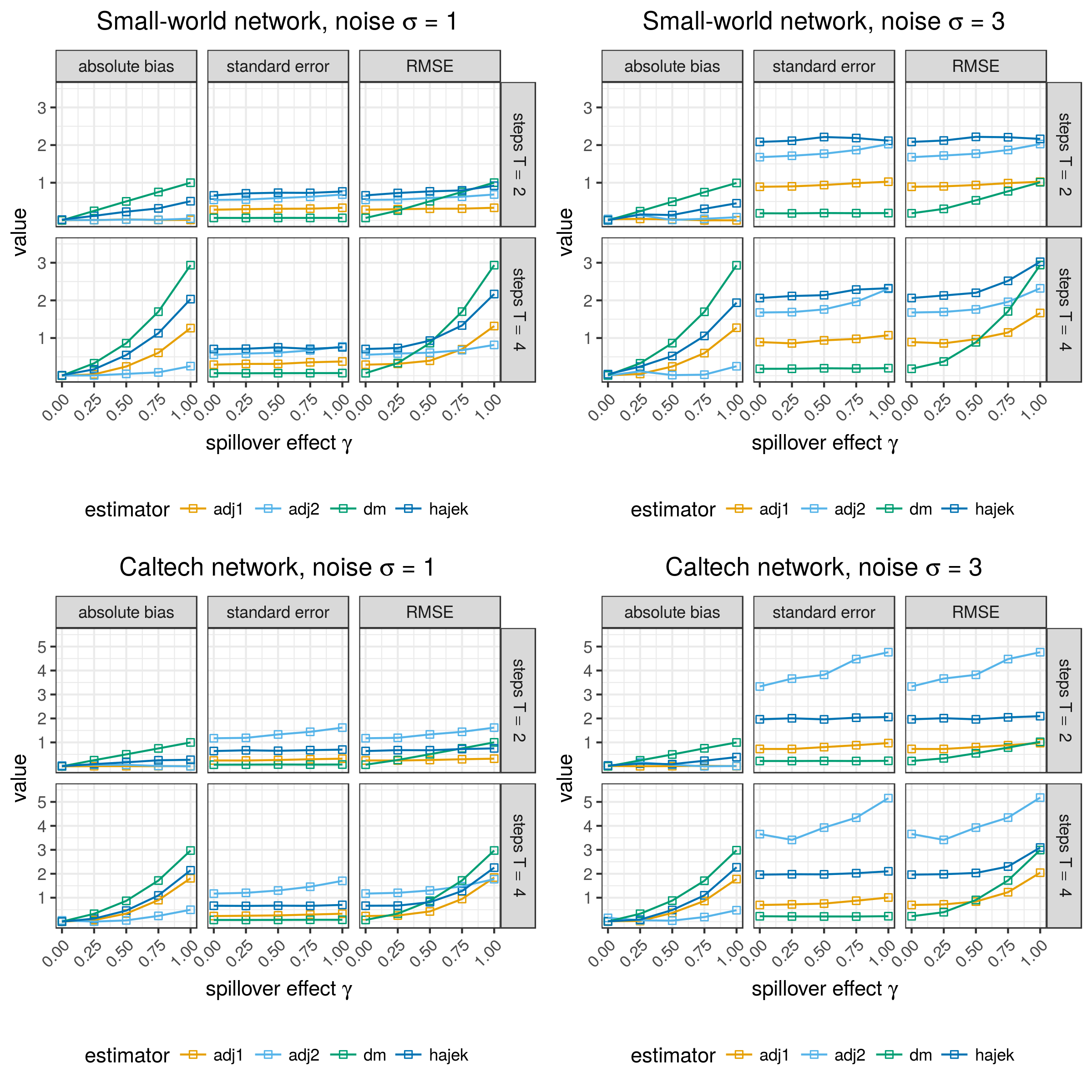
The difference-in-means estimator outperforms the adjustment estimators in regimes of weak interference, which is expected since difference-in-means is the best that can be done under correct specification of SUTVA. In terms of RMSE the Hájek estimator sometimes outperforms the two-step adjustment estimator because of large variance. However, if the main goal is robustness to interference, then unconfounded estimation coupled with valid confidence intervals is likely the priority over optimizing an error metric such as RMSE. In this case, since the Hájek estimator neither achieve sufficient bias reduction nor provide correct coverage, it has no real advantage over the adjustment estimators.
Figure 5 displays the coverage rates obtain from variance estimates using equation (17) under the dynamic treatment response setup. The coverage is not always correct due to misspecification, especially for adj1. We see that coverage rates for adj2 are often conservative even though it too is misspecified. We note that standard variance estimators for the difference-in-means estimator and those derived in Aronow and Samii [2017] for the Hájek estimator also would fail here because they rely on correct specification of SUTVA and an exposure model, respectively. In short, we are plagued with the same difficulties that beset attempting to do valid inference in observational studies when we do not know whether unconfoundedness holds.

5.5 Average + aggregate peer effects
In this example we consider a response model in which individuals respond partially to the average behavior of their peers and partially to the aggregate behavior of their peers. Let
be the fraction of treated neighbors and
be the number of treated neighbors. captures a notion of fractional neighborhood exposure and captures a notion of absolute neighborhood exposure. It seems reasonable that both of these features may contribute interference. In order to use an exposure model estimator one would need to focus on either fractional exposure or absolute exposure, or otherwise define a more complicated exposure model, but our adjustments easily handle both features.
We consider the following response function:
where introduces heterogeneity into the direct effect and is homoscedastic noise. This function captures a possible way in which individuals could respond nonlinearly to their peer exposures through and . Figure 6 plots a single draw of this response on individuals from the Stanford network. The continuous response exhibits a logistic dependence on both features. We see that individuals with less than half of their neighbors exposed to the treatment condition experience a steadily increasing peer effect as the proportion of treated neighbors increases. For individuals with more than half of their neighbors exposed to the treatment condition, the effect is nearly constant across values of , capturing the idea that after a certain threshold observing additional peer exposures doesn’t add much. For , we see that a small number of treated neighbors essentially contributes no interference, but once a large number of neighbors are exposed to treatment this has a measurable impact on the response. We also see that there is a noticeable bump around ; this is because individuals with peers nearly equally assigned to the two groups are more likely to have high degree. The model extends the idea of neighborhood exposure to capture the intuition that having a high proportion of treated neighbors is evidence for being subject to interference, but such evidence is stronger when the individual in question has many friends and not just one or two friends. The true treatment effect is , which was computed using 2000 Monte Carlo draws each of global treatment and global control.

In our experience larger populations seem to be needed for fitting the more complex, nonlinear functions, so we work with the Stanford network which has 11586 nodes. We predict the response surfaces using a generalized additive model (GAM) [Hastie and Tibshirani 1986], which is easy and fast to fit in R, but other methods such as local regression or random forests could of course be used instead. We split the dataset into folds, and within each fold, train a GAM separately in the treatment and control groups for a total of 4 fitted models. The models are then used to obtain predicted responses on the held-out fold. Standard errors were computed via the bootstrap as described in Section 4.1, using 50 bootstrap replications.
We compare to the difference-in-means estimator, the Hájek estimator using a threshold of on the variable, and the OLS adjustment. The results are displayed in Table 3. The DM estimator exhibits the most bias, as it does not adjust for any sort of interference. The Hájek estimator removes some bias, but because it is based on a fractional exposure model it is unable to respond to the effect of having a high treated degree. Both the OLS and GAM estimators remove about 95% of the bias. The GAM adjustment does only slightly better than OLS; for this setup what matters most is adjusting for both axes of the interference statistic, and the added flexibility provided by the GAM does not seem to be crucial. We note also that average bootstrapped standard error is 1.076 times greater than the true standard error, suggesting that confidence intervals built on this standard error will have the approximately correct length.
| estimator | estimate | absolute bias (%) | SE (ratio) |
|---|---|---|---|
| DM | -0.002 | 6.339 (100%) | 0.077 (—) |
| Hájek | 2.653 | 3.683 (58.1%) | 1.601 (—) |
| OLS | 6.683 | 0.347 (5.5%) | 0.252 (0.942) |
| GAM | 6.655 | 0.319 (5.0%) | 0.246 (1.076) |
6 Application to a farmer’s insurance experiment
In this section we apply our methods to a field experiment conducted on individuals in 185 villages in rural China [Cai et al. 2015]. The purpose of the study was to quantify the network (spillover) effects of certain information sessions for a farmer’s weather insurance product on the eventual adoption of that product. Though they do not frame their approach explicitly in the language of exposure models as in [Aronow and Samii 2017], the estimands that are implied by the regression coefficients in the models that they use in that paper can be thought of as contrasts between exposures in an appropriately-defined exposure model. The authors did not consider estimating the global treatment effect; our proposed methods essentially allow us to perform an off-policy analysis of that estimand.
In the original field experiment, the researchers consider four treatment groups obtained by assigning villagers to either a simple or intensive information session in one of two rounds that were held three days apart. Here, for simplicity, we ignore the temporal distinction between the two rounds and consider a villager to be treated if they were exposed to either of the two intensive sessions.33 3 According to Cai et al. [2015] the treatment groups in the study are stratified by household size and farm size, but it is not clear from the data if and how exactly this was done, so for simplicity we analyze the experiment as if it were an unstratified, Bernoulli randomized experiment. The outcome variable is a binary indicator for whether the villager decided to purchase weather insurance.
We drop all villagers that were missing information about the treatment or the response, as well as villages lacking network information. Though the study was conducted in separate villages (for the purpose of administering the insurance information sessions), we combine all of the villagers into one large graph . The network has 4,382 nodes and 17,069 edges. Because some social connections exist across villages, the villages do not partition exactly into separate connected components; our graph has 36 connected components. The summary statistics for the processed dataset are given in Table 4.
| number of nodes | 4832 |
|---|---|
| number of edges | 17069 |
| number (%) treated | 2406 (49.8%) |
| average takeup (mean response) | 44.6% |
Now let and be the one- and two-step neighborhoods for unit , as we have denoted previously. We construct four variables from the graph: the fraction of units in who are treated (frac1), the fraction of units in who are treated (frac2), the number of units in who are treated (num1), and the number of units in who are treated (num2). Figure 7 displays the scatterplot matrix for these four variables as well as the response. As might be expected, these four variables are positively correlated with each other, and each is (weakly) positively correlated with the response variable. This correlation with the response suggests that these variables may be useful for adjustment.

We compute the OLS adjusted estimator as well as an adjustment estimator that used predictions from a logistic regression with folds. We construct standard errors using the variance estimator given by equation (17) in the OLS case, and the parametric bootstrap variance estimator described in Section 4.1 with 200 bootstrap replications for the logistic regression case. We compare to the difference-in-means estimator and Hájek estimators based on thresholding on the frac1 and frac2 variables with .
The estimates are displayed in Table 5. Considering the strong positive spillover effects discovered by Cai et al. [2015], the difference-in-means estimate of 0.0774 is likely to be an underestimate of the true global treatment effect. The Hájek estimators produce estimates of 0.1630 (one-step fractional NTR) and 0.1672 (two-step fractional NTR). Though we do not know the truth, it may make us nervous that these estimates are more than twice the magnitude of the difference-in-means estimator, which if true would suggest that magnitude of the spillover effect is larger than the magnitude of the direct effect. The true treatment effect likely falls in between the estimates produced by difference-in-means and Hájek (though we have no way of knowing for sure). The OLS (0.1218) and logistic regression estimates (0.1197) are similar to each other and both within this range; an advantage they have over the Hájek estimators is that they incorporate information about the raw number of treated neighbors. The standard error estimates of 0.0561 (linear regression adjustment) and 0.0559 (logistic regression adjustment) are quite wide, suggesting some caution when interpreting this result.
Note that we have omitted computation of standard error estimates for the difference-in-means and Hájek estimators for several reasons. SUTVA and the neighborhood exposure conditions both likely fail to hold, so it is unclear how we should interpret such standard errors. Secondly, the conservative variance estimators proposed for the Hájek estimator [Aronow and Samii 2017, cf. Sections 5, 7.2,] are themselves inverse propensity estimators relying on small propensities, and consequently we found them to be quite unstable. For example, the variance estimate was often much greater than 1, which is the maximum possible variance of a -valued random variable. Of course, we also do not know if the exogeneity assumptions hold or if other variables should be included. In the regression analyses conducted by Cai et al. [2015], they also consider some other social network measures including indicator variables for varying numbers of friends and differentiation between strong and weak ties; a more sophisticated analysis here could include these features as well.
| estimator | estimate | standard error |
|---|---|---|
| DM | 0.0774 | — |
| Hájek 1 () | 0.1630 | — |
| Hájek 2 () | 0.1672 | — |
| Linear | 0.1218 | 0.0561 |
| Logistic (5-fold) | 0.1197 | 0.0559 |
7 Discussion
We propose regression adjustments for interference in randomized experiments, which opens the world of the rich regression adjustment literature to the interference setting. We show in simulation experiments that the adjustments can do well, and we show how to do inference under exogeneity/unconfoundedness assumptions. Our reanalysis of the Cai et al. [2015] study shows that our approach can produce sensible estimates of the global treatment effect on real data.
There is much work to do to ensure that this approach can be reliably used in practical settings. First, we would like to extend the methods to handle more complicated designs. In reality a combination of design-side methods (graph clustering) and analysis-side methods (adjustment) could be the most effective approach. It would also be useful to have a thorough understanding of the combinations of network structures and experimental designs that correspond to the mathematical assumptions (exogeneity, full-rank design) listed in this paper.
Secondly, it is necessary to formalize the placement of the methods discussed here within the agnostic perspective to treatment effect estimation. This would clarify the exogeneity/unconfoundedness requirement and better elucidate how interference causes a randomized experiment to behave in some ways like an observational study. However, such assumptions are not new, and also needed to employ both standard estimators for observational studies in the SUTVA setting and exposure modeling estimators in the interference setting.
This issue simply highlights the need for better methods that can detect interference; there are several budding possibilities here. First, several works have proposed ways of doing sensitivity analysis for interference. VanderWeele et al. [2014] extend Robins et al. [2000]-style sensitivity analysis to cover some of the interference estimators studied in Hudgens and Halloran [2008], and Egami [2017] propose using an auxiliary network to perform sensitivity analysis on estimates obtained using the primary network. But clearly more work in this area is needed. Second, hypothesis tests for network or spillover effects of the type developed in [Aronow 2012, Athey et al. 2017a, Basse et al. 2017], could be informative if applied to the residuals of a fitted interference model. Finally, one can always use more robust standard error constructions such as Eicker-Huber-White [Eicker 1967, Huber 1967, White 1980] standard errors for heteroscedasticity or cluster bootstrap methods for dependence, though if the network structure is such that graph cluster randomization is unlikely to work well, then clustered bootstrap probably won’t work well either. It is also possible that work based on dependency central limit theorems like the ones considered in Chin [2018] could be used to develop more robust variance calculations. Broadly, any of the above methods ideas can be applied to the residuals of an interference model. If the bulk of interference can be captured in the mean function, then it is perhaps easier to deal with the remaining interference in the residuals.
References
- Abadie et al. [2017a] A. Abadie, S. Athey, G. W. Imbens, and J. Wooldridge. When should you adjust standard errors for clustering? Technical report, National Bureau of Economic Research, 2017a.
- Abadie et al. [2017b] A. Abadie, S. Athey, G. W. Imbens, and J. M. Wooldridge. Sampling-based vs. design-based uncertainty in regression analysis. arXiv preprint arXiv:1706.01778, 2017b.
- Aral [2016] S. Aral. Networked experiments. Oxford, UK: Oxford University Press, 2016.
- Aronow [2012] P. M. Aronow. A general method for detecting interference between units in randomized experiments. Sociological Methods & Research, 41(1):3–16, 2012.
- Aronow and Middleton [2013] P. M. Aronow and J. A. Middleton. A class of unbiased estimators of the average treatment effect in randomized experiments. Journal of Causal Inference, 1(1):135–154, 2013.
- Aronow and Samii [2017] P. M. Aronow and C. Samii. Estimating average causal effects under general interference, with application to a social network experiment. The Annals of Applied Statistics, 11(4):1912–1947, 2017.
- Athey et al. [2017a] S. Athey, D. Eckles, and G. W. Imbens. Exact -values for network interference. Journal of the American Statistical Association, pages 1–11, 2017a.
- Athey et al. [2017b] S. Athey, G. W. Imbens, and S. Wager. Approximate residual balancing: De-biased inference of average treatment effects in high dimensions. 2017b. URL: https://arxiv.org/pdf/1604.07125.pdf.
- Backstrom et al. [2012] L. Backstrom, P. Boldi, M. Rosa, J. Ugander, and S. Vigna. Four degrees of separation. In Proceedings of the 4th Annual ACM Web Science Conference, pages 33–42. ACM, 2012.
- Baird et al. [2016] S. Baird, J. A. Bohren, C. McIntosh, and B. Özler. Optimal design of experiments in the presence of interference. Review of Economics and Statistics, (0), 2016.
- Banerjee et al. [2013] A. Banerjee, A. G. Chandrasekhar, E. Duflo, and M. O. Jackson. The diffusion of microfinance. Science, 341(6144):1236498, 2013.
- Basse and Feller [2018] G. Basse and A. Feller. Analyzing two-stage experiments in the presence of interference. Journal of the American Statistical Association, 113(521):41–55, 2018.
- Basse et al. [2017] G. Basse, A. Feller, and P. Toulis. Exact tests for two-stage randomized designs in the presence of interference. arXiv preprint arXiv:1709.08036, 2017.
- Beaman et al. [2018] L. Beaman, A. BenYishay, J. Magruder, and A. M. Mobarak. Can network theory-based targeting increase technology adoption? Technical report, National Bureau of Economic Research, 2018.
- Berk et al. [2013] R. Berk, E. Pitkin, L. Brown, A. Buja, E. George, and L. Zhao. Covariance adjustments for the analysis of randomized field experiments. Evaluation Review, 37(3-4):170–196, 2013.
- Bhagat et al. [2016] S. Bhagat, M. Burke, C. Diuk, I. O. Filiz, and S. Edunov. Three and a half degrees of separation. Facebook research note, 2016. URL: https://research.fb.com/three-and-a-half-degrees-of-separation/.
- Bloniarz et al. [2016] A. Bloniarz, H. Liu, C.-H. Zhang, J. S. Sekhon, and B. Yu. Lasso adjustments of treatment effect estimates in randomized experiments. Proceedings of the National Academy of Sciences, 113(27):7383–7390, 2016.
- Blume [1995] L. E. Blume. The statistical mechanics of best-response strategy revision. Games and Economic Behavior, 11(2):111–145, 1995.
- Bramoullé et al. [2009] Y. Bramoullé, H. Djebbari, and B. Fortin. Identification of peer effects through social networks. Journal of Econometrics, 150(1):41–55, 2009.
- Cai et al. [2015] J. Cai, A. De Janvry, and E. Sadoulet. Social networks and the decision to insure. American Economic Journal: Applied Economics, 7(2):81–108, 2015.
- Chen and Lei [2018] K. Chen and J. Lei. Network cross-validation for determining the number of communities in network data. Journal of the American Statistical Association, 113(521):241–251, 2018.
- Chernozhukov et al. [2018] V. Chernozhukov, D. Chetverikov, M. Demirer, E. Duflo, C. Hansen, W. Newey, and J. Robins. Double/debiased machine learning for treatment and structural parameters. The Econometrics Journal, 21(1):C1–C68, 2018.
- Chin [2018] A. Chin. Central limit theorems via Stein’s method for randomized experiments under interference. arXiv preprint arXiv:1808.08683, 2018.
- Choi [2017] D. Choi. Estimation of monotone treatment effects in network experiments. Journal of the American Statistical Association, pages 1–9, 2017.
- Cox [1958] D. R. Cox. Planning of experiments. 1958.
- Eckles et al. [2017] D. Eckles, B. Karrer, and J. Ugander. Design and analysis of experiments in networks: Reducing bias from interference. Journal of Causal Inference, 5(1), 2017.
- Efron [1979] B. Efron. Bootstrap methods: Another look at the jackknife. The Annals of Statistics, 7(1):1–26, 1979.
- Efron [1987] B. Efron. Better bootstrap confidence intervals. Journal of the American Statistical Association, 82(397):171–185, 1987.
- Egami [2017] N. Egami. Unbiased estimation and sensitivity analysis for network-specific spillover effects: Application to an online network experiment. arXiv preprint arXiv:1708.08171, 2017.
- Eicker [1967] F. Eicker. Limit theorems for regressions with unequal and dependent errors. 1967.
- Forastiere et al. [2016] L. Forastiere, E. M. Airoldi, and F. Mealli. Identification and estimation of treatment and interference effects in observational studies on networks. arXiv preprint arXiv:1609.06245, 2016.
- Fortunato [2010] S. Fortunato. Community detection in graphs. Physics reports, 486(3-5):75–174, 2010.
- Freedman [2008a] D. A. Freedman. On regression adjustments to experimental data. Advances in Applied Mathematics, 40(2):180–193, 2008a.
- Freedman [2008b] D. A. Freedman. On regression adjustments in experiments with several treatments. The annals of applied statistics, 2(1):176–196, 2008b.
- Fruchterman and Reingold [1991] T. M. Fruchterman and E. M. Reingold. Graph drawing by force-directed placement. Software: Practice and Experience, 21(11):1129–1164, 1991.
- Granovetter [1973] M. S. Granovetter. The strength of weak ties. American Journal of Sociology, 78(6):1360–1380, 1973.
- Greenland [1987] S. Greenland. Interpretation and choice of effect measures in epidemiologic analyses. American journal of epidemiology, 125(5):761–768, 1987.
- Hahn [1998] J. Hahn. On the role of the propensity score in efficient semiparametric estimation of average treatment effects. Econometrica, pages 315–331, 1998.
- Hájek [1971] J. Hájek. Comment on ‘An essay on the logical foundations of survey sampling, part 1’ by D. Basu. In V. Godambe and D. A. Sprott, editors, Foundations of Statistical Inference, page 236, Toronto, 1971. Holt, Rinehart and Winston.
- Hastie and Tibshirani [1986] T. Hastie and R. Tibshirani. Generalized additive models. Statistical Science, 1(3):297–310, 1986.
- Haythornthwaite and Wellman [1998] C. Haythornthwaite and B. Wellman. Work, friendship, and media use for information exchange in a networked organization. Journal of the American society for information science, 49(12):1101–1114, 1998.
- Horvitz and Thompson [1952] D. G. Horvitz and D. J. Thompson. A generalization of sampling without replacement from a finite universe. Journal of the American Statistical Association, 47(260):663–685, 1952.
- Huber [1967] P. J. Huber. The behavior of maximum likelihood estimates under nonstandard conditions. 1967.
- Hudgens and Halloran [2008] M. G. Hudgens and M. E. Halloran. Toward causal inference with interference. Journal of the American Statistical Association, 103(482):832–842, 2008.
- Imbens [2004] G. W. Imbens. Nonparametric estimation of average treatment effects under exogeneity: A review. Review of Economics and Statistics, 86(1):4–29, 2004.
- Jagadeesan et al. [2017] R. Jagadeesan, N. Pillai, and A. Volfovsky. Designs for estimating the treatment effect in networks with interference. arXiv preprint arXiv:1705.08524, 2017.
- Kim et al. [2015] D. A. Kim, A. R. Hwong, D. Stafford, D. A. Hughes, A. J. O’Malley, J. H. Fowler, and N. A. Christakis. Social network targeting to maximise population behaviour change: a cluster randomised controlled trial. The Lancet, 386(9989):145–153, 2015.
- Kivelä et al. [2014] M. Kivelä, A. Arenas, M. Barthelemy, J. P. Gleeson, Y. Moreno, and M. A. Porter. Multilayer networks. Journal of Complex Networks, 2(3):203–271, 2014.
- Künsch [1986] H. R. Künsch. The jackknife and the bootstrap for general stationary observations. The Annals of Statistics, pages 1217–1241, 1989.
- Li et al. [2018] T. Li, E. Levina, and J. Zhu. Network cross-validation by edge sampling. arXiv preprint arXiv:1612.04717, 2018.
- Lin [2013] W. Lin. Agnostic notes on regression adjustments to experimental data: Reexamining Freedman’s critique. The Annals of Applied Statistics, 7(1):295–318, 2013.
- Liu and Hudgens [2014] L. Liu and M. G. Hudgens. Large sample randomization inference of causal effects in the presence of interference. Journal of the American Statistical Association, 109(505):288–301, 2014.
- Manski [1993] C. F. Manski. Identification of endogenous social effects: The reflection problem. The Review of Economic Studies, 1993.
- Manski [2013] C. F. Manski. Identification of treatment response with social interactions. The Econometrics Journal, 16(1), 2013.
- Neyman [1923] J. Neyman. On the application of probability theory to agricultural experiments. Essay on Principles. section 9. (translated and edited by D. M. Dabrowska and T. P. Speed, Statistical Science (1990), 5, 465-480). Annals of Agricultural Sciences, 10:1–51, 1923.
- Ogburn and VanderWeele [2014] E. L. Ogburn and T. J. VanderWeele. Causal diagrams for interference. Statistical Science, 29(4):559–578, 2014.
- Paluck et al. [2016] E. L. Paluck, H. Shepherd, and P. M. Aronow. Changing climates of conflict: A social network experiment in 56 schools. Proceedings of the National Academy of Sciences, 113(3):566–571, 2016.
- Pearl [2009] J. Pearl. Causality. Cambridge University Press, 2009.
- Robins and Greenland [1989] J. Robins and S. Greenland. The probability of causation under a stochastic model for individual risk. Biometrics, pages 1125–1138, 1989.
- Robins and Greenland [2000] J. M. Robins and S. Greenland. Causal inference without counterfactuals: comment. Journal of the American Statistical Association, 95(450):431–435, 2000.
- Robins et al. [2000] J. M. Robins, A. Rotnitzky, and D. O. Scharfstein. Sensitivity analysis for selection bias and unmeasured confounding in missing data and causal inference models. In Statistical Models in Epidemiology, the Environment, and Clinical Trials, pages 1–94. Springer, 2000.
- Rosenbaum [2007] P. R. Rosenbaum. Interference between units in randomized experiments. Journal of the American Statistical Association, 102(477):191–200, 2007.
- Rubin [1974] D. B. Rubin. Estimating causal effects of treatments in randomized and nonrandomized studies. Journal of Educational Psychology, 66(5):688, 1974.
- Rubin [1980] D. B. Rubin. Randomization analysis of experimental data: The Fisher randomization test comment. Journal of the American Statistical Association, 1980.
- Saveski et al. [2017] M. Saveski, J. Pouget-Abadie, G. Saint-Jacques, W. Duan, S. Ghosh, Y. Xu, and E. M. Airoldi. Detecting network effects: Randomizing over randomized experiments. In Proceedings of the 23rd ACM SIGKDD International Conference on Knowledge Discovery and Data Mining, pages 1027–1035. ACM, 2017.
- Sävje et al. [2017] F. Sävje, P. M. Aronow, and M. G. Hudgens. Average treatment effects in the presence of unknown interference. arXiv preprint arXiv:1711.06399, 2017.
- Sussman and Airoldi [2017] D. L. Sussman and E. M. Airoldi. Elements of estimation theory for causal effects in the presence of network interference. arXiv preprint arXiv:1702.03578, 2017.
- Taylor and Eckles [2017] S. J. Taylor and D. Eckles. Randomized experiments to detect and estimate social influence in networks. arXiv preprint arXiv:1709.09636, 2017.
- Tchetgen Tchetgen and VanderWeele [2012] E. J. Tchetgen Tchetgen and T. J. VanderWeele. On causal inference in the presence of interference. Statistical methods in medical research, 21(1):55–75, 2012.
- Traud et al. [2011] A. L. Traud, E. D. Kelsic, P. J. Mucha, and M. A. Porter. Comparing community structure to characteristics in online collegiate social networks. SIAM review, 53(3):526–543, 2011.
- Traud et al. [2012] A. L. Traud, P. J. Mucha, and M. A. Porter. Social structure of Facebook networks. Physica A: Statistical Mechanics and its Applications, 391(16):4165–4180, 2012.
- Tyner et al. [2017] S. Tyner, F. Briatte, and H. Hofmann. Network visualization with ggplot2. The R Journal, 2017.
- Ugander and Backstrom [2013] J. Ugander and L. Backstrom. Balanced label propagation for partitioning massive graphs. In Proceedings of the sixth ACM International Conference on Web Search and Data Mining, pages 507–516. ACM, 2013.
- Ugander et al. [2011] J. Ugander, B. Karrer, L. Backstrom, and C. Marlow. The anatomy of the Facebook social graph. arXiv preprint arXiv:1111.4503, 2011.
- Ugander et al. [2013] J. Ugander, B. Karrer, L. Backstrom, and J. Kleinberg. Graph cluster randomization: Network exposure to multiple universes. In Proceedings of the 19th ACM SIGKDD International Conference on Knowledge Discovery and Data Mining, pages 329–337. ACM, 2013.
- van der Laan [2014] M. J. van der Laan. Causal inference for a population of causally connected units. Journal of Causal Inference, 2(1):13–74, 2014.
- VanderWeele and Robins [2012] T. J. VanderWeele and J. M. Robins. Stochastic counterfactuals and stochastic sufficient causes. Statistica Sinica, 22(1):379, 2012.
- VanderWeele and Tchetgen Tchetgen [2011] T. J. VanderWeele and E. J. Tchetgen Tchetgen. Effect partitioning under interference in two-stage randomized vaccine trials. Statistics & Probability Letters, 81(7):861–869, 2011.
- VanderWeele et al. [2014] T. J. VanderWeele, E. J. Tchetgen Tchetgen, and M. E. Halloran. Interference and sensitivity analysis. Statistical Science: A review journal of the Institute of Mathematical Statistics, 29(4):687, 2014.
- Wager et al. [2016] S. Wager, W. Du, J. Taylor, and R. J. Tibshirani. High-dimensional regression adjustments in randomized experiments. Proceedings of the National Academy of Sciences, 113(45):12673–12678, 2016.
- Walker and Muchnik [2014] D. Walker and L. Muchnik. Design of randomized experiments in networks. Proceedings of the IEEE, 102(12):1940–1951, 2014.
- Watts and Strogatz [1998] D. J. Watts and S. H. Strogatz. Collective dynamics of ‘small-world’ networks. Nature, 393(6684):440, 1998.
- White [1980] H. White. A heteroskedasticity-consistent covariance matrix estimator and a direct test for heteroskedasticity. Econometrica: Journal of the Econometric Society, pages 817–838, 1980.
- Wu [1986] C.-F. J. Wu. Jackknife, bootstrap and other resampling methods in regression analysis. The Annals of Statistics, pages 1261–1295, 1986.
- Wu and Gagnon-Bartsch [2017] E. Wu and J. Gagnon-Bartsch. The LOOP estimator: Adjusting for covariates in randomized experiments. arXiv preprint arXiv:1708.01229, 2017.
Appendix A Proofs for Section 3
A.1 Proof of Proposition 1
A.2 Proof of Theorem 1
A.3 Proof of Theorem 2
This lemma establishes some basic convergence results.
Lemma 1.
Proof.
- (a)
Because of Bernoulli random sampling it holds that
By conditioning on we have
For the first term, we have
where
and
since in probability. For the second term, we have
since . Therefore, we conclude , and so consistency follows from Chebychev’s inequality.
The result similarly holds for .
- (b)
This result is established in a similar manner to part (a), using the fact that
and the fact that fourth moments are bounded.
- (c)
The convergence of to follows conditionally on from standard OLS theory. Then, letting
denote the sample covariance matrix, we find
Convergence in probability follows from Chebychev’s inequality.
- (d)
This result follows from Bernoulli sampling and the convergence of the finite population means, .
- (e)
As in the proof of part (c), we write
Since , we can write
where the remainder is
Since is implied by , and and , the remainder satisfies .
Then is asymptotically Gaussian with mean zero and variance
Using the result of part (d), this variance equals when and when .
- (f)
From Assumption 3, is independent of with variances and , respectively. A standard central limit theorem shows that is asymptotically Gaussian with mean and variance
∎
We now prove the main theorem.
Proof.
We characterize the treatment effect estimator as
which implies that
Now,
for , where the second term is since and following from parts (a) and (c) of Lemma 1. Therefore,
A.4 Proof of Corollary 1
Proof.
If is independent of , then
and so is equal to in the limit (with the understanding that is actually a sequence associated with each finite population). The same holds true for . Then the result follows immediately from equation (19), as the second and third terms are equal to zero. ∎