Superconductivity near a nematic quantum critical point – the interplay between hot and lukewarm regions
Abstract
We present a strong coupling dynamical theory of the superconducting transition in a metal near a QCP towards nematic order. We use a fermion-boson model, in which we treat the ratio of effective boson-fermion coupling and the Fermi energy as a small parameter . We solve, both analytically and numerically, the linearized Eliashberg equation. Our solution takes into account both strong fluctuations at small momentum transfers and weaker fluctuations at large momentum transfers. The strong fluctuations determine , which is of order for both and wave pairing. The weaker fluctuations determine the angular structure of the superconducting order parameter along the Fermi surface, separating between hot and lukewarm regions. In the hot regions is largest and approximately constant. Beyond the hot region, whose width is , drops by a factor . The and wave states are not degenerate but the relative difference is small.
Introduction
Superconductivity (SC) mediated by fluctuations arising from proximity to an electronic quantum-critical point (QCP) has attracted tremendous interest in the “high ” era. Much of the motivation comes from the known proximity of the Cu- and Fe- based superconductors to antiferromagnetism [1, 2, 3, 4, 5, 6] but more recent discoveries of charge-density-wave order in the cuprates and of nematic order in both Cu-and Fe-based materials[7, 8, 9] have led to studies of SC mediated by critical charge fluctuations [10, 11, 12]. Theoretical studies of SC near a QCP show that it is a strong coupling phenomenon, arising from the divergent fluctuations [13, 14, 15]. These fluctuations also induce large electronic self-energies, which in the absence of SC would account for a non Fermi liquid (NFL) behavior below some characteristic frequency [16, 13, 3, 17, 18, 19, 20, 21]. In some systems SC emerges at and masks the NFL behavior [22, 15], in other systems is smaller than , at least numerically. In the latter case SC emerges out of a NFL.
A subset of theories of SC in a quantum-critical regime are those dealing with transitions at vanishing momentum transfer [23, 16, 24, 25, 26, 17, 27, 28, 21, 15, 22]. They are typically associated with a deformation of the Fermi surface (FS) in some angular momentum channel, e.g. for the nematic transition of the type observed in Fe- and Cu-based SCs. A theory of pairing mediated by soft fluctuations of wave nematic order parameter must account both for the strong coupling physics that occurs locally on the Fermi surface (FS), and for the momentum anisotropy caused by a wave form-factor, which occurs on the large momentum scale of the Fermi wavevector .
This paper deals with SC at the nematic QCP. The form of the wave form-factor splits the FS into four ‘hot’ regions where , , where interactions are strong, and four ‘lukewarm’ regions where , where the pairing interaction is much weaker [29, 30]. Previous studies of this problem have focused either on the pairing away from a QCP within a Fermi liquid framework [29], or on local strong-coupling properties in the hot regions [15, 31, 22, 14, 32], where the interaction is at its maximum, but doesn’t distinguish between pairing channels. These studies found that is comparable to the upper boundary of the NFL behavior. The weak coupling FL study focused on the angular variation of the gap along the whole FS and on the difference between the pairing strength in different spin-singlet pairing channels. This study found that at a finite distance from a nematic transition (measured by the inverse correlation length of nematic fluctuations) wave pairing wins over wave and higher symmetry channels, but the splitting between the coupling strength in different channels scales as and vanishes at a QCP. That work also found that, at a finite , there are two scales in the problem: the relevant momentum transfer in the gap equation is of order , but the gap varies at a larger scale . In the FL description, both scales collapse when diverges.
Our work unifies the strong coupling and weak coupling approaches. We analyze the pairing near a nematic QCP including both the angular dependence of the nematic form-factor along the FS and the dynamics of the pairing interaction and associated self-energy . We obtain in different pairing channels and the angular variation of the pairing gap by solving the linearized Eliashberg gap equation right at a QCP, where . We argue that the gap variation along the FS and the difference between the couplings in wave and wave channels are governed by a single dimensionless parameter , which is the ratio of the effective boson-fermion coupling and the Fermi energy, which we assume to be of order bandwidth. At a metallic QCP, interaction is assumed to be smaller than the bandwidth, and we treat as a small parameter.
We show that remains finite at a QCP, and wave and wave channels remain non-degenerate. The difference between the two comes from the dynamical part of the pairing interaction. The for wave pairing is higher, and the difference . We show that the angular dependence of the form-factor causes a sharp angular variation of the pairing gap along the FS in both and channels as a function of distance along the FS from where the form factor is maximal (i.e., from ). The pairing gap is the largest in “hot” regions with a width of order . This scale is parametrically larger than the typical momentum transfer by the interaction, , but smaller than typical scale of variation of the form-factor, which is . Between the two scales the gap behaves as . This behavior holds for both wave and wave pairing gaps, and the difference between the two develops at .
The Model.
We base our study on the standard boson-fermion coupling model [33, 34, 16]. The bosons represent some collective degree of freedom, either charge excitations near a Pomeranchuk instability, or some composite spin fluctuations responsible for d-wave nematic order. We assume a circular FS and dispersion , but a generalization to a more general FS is straightforward. The wave symmetry of a nematic order is encoded in the fermion-boson interaction,
| (1) |
in which represents the wave form-factor and is a bosonic field with static propagator . At a QCP, . The effective boson-fermion interaction is and the dimensionless coupling . In our problem, the relevant degrees of freedom are near the FS, so we approximate by an angular function .
We use as an input the result of earlier studies [3, 35, 17, 36, 37] that to leading order in fermionic and bosonic self-energies are given by one-loop expressions with free-fermion propagators. The bosonic self-energy gives rise to Landau damping and changes the bosonic propagator at a QCP to
| (2) |
where and is the effective coupling. For fermions at the FS, the momentum transfer is , and the susceptibility becomes the function of only and . The fermionic self-energy near the FS is
| (3) |
where . The form is a result of the scaling.
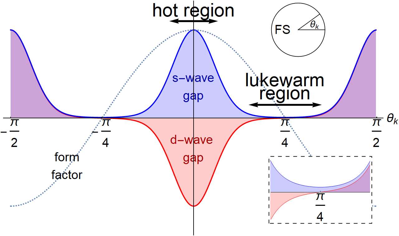
The Eliashberg equation.
In order to obtain the linearized Eliashberg equation for the anomalous pair function we consider the ladder series of diagrams for infinitesimally small with as the interaction and use full fermionic propagators with the self-energy . The Eliashberg equation is obtained by approximating the pairing interaction by that for fermions right on the FS (i.e., approximating by and integrating out the momentum transverse to the FS in the fermionic propagators. This is justified because typical bosonic momenta are parametrically larger than typical fermionic momenta for and for . Integrating over the momentum transverse to the FS we obtain
| (4) |
where we defined explicitly
| (5) |
Notice that this is a 2D integral equation in both frequency and the angle along the FS. We removed the thermal contribution , as it does not affect for spin-singlet pairing [13, 38, 39], similar to the effect to non-magnetic impurities [40, 41]. Note that because and , Eq. (4) depends on a single parameter , when is rescaled by .
Eq. (4) has a straightforward interpretation. The term is the result of integrating out the fermionic particle-particle bubble, that for a constant interaction would give the usual BCS form of the gap equation. The term on the second line is the bosonic susceptibility, weighted by the vertex form-factors, and is momentum variation between two points on the FS separated by an angle . For small angles, . Because of factor in various places in the Eliashberg equation, the FS can be segmented into ‘hot’ regions, where , and ‘lukewarm’ regions where . Fig. 1 depicts the behavior of the form-factor and shows the hot and lukewarm regions of the FS.
and the angular variation of .
We first obtain . The frequency sum over in (4) is UV convergent, hence typical and are of the same order of Typical are then of order . We will see that in our case . Then typical are of order . The wave form-factor does not vary on such scale and can be set to . We assume and then verify that also varies slowly at and can be approximated by . In this situation we can integrate over in (4) and obtain a local gap equation,
| (6) |
where
| (7) |
Eq. (6) is dimensionless, local, and universal in the sense that dimensionless cancels out. Solving Eq. (6) numerically, we find
| (8) |
This is consistent [42] with earlier works [23, 32, 14, 21, 43].
We next look at a lukewarm region and examine whether the interaction within this region can give rise to a comparable . For definiteness let’s focus on near . In lukewarm regions we need to differentiate between -wave and wave (even and odd) solutions with , where . Because , the effective static boson-mediated interaction is not singular and weak. In this situation, one can neglect both the Landau damping and the fermionic self-energy. Then does not depend on , i.e., the pairing is described by BCS theory, with an onset temperature , where . The temperature is indeed much smaller than in Eq. (8), and the same holds for d-wave pairing. This implies that s-wave SC in a lukward region is induced by that in the hot regions.
We now determine the angular variation of the gap in the hot regions. For definiteness consider the segment . We label a characteristic at which varies as . At a first glance, should be of order one because varies at . However, we show that is actually parametrically smaller and is of order . To see this, we assume that and then verify it. Because typical and in the Eliashberg equation are of order , i.e., and , we can reduce the 2D integral equation (4) to a 1D equation on :
| (9) |
If we approximate by and and by , we see that Eq. (9) reduces to an identity, as should be for . Going beyond this approximation, we expand in (9) as .For the second term in is irrelevant by construction, but for it plays a major role. Indeed, for these there are two contributions to the r.h.s. of (9). One comes from the integration over a narrow range and yields . The other comes from the coupling to hot region, where . Typical for this second contribution are , i.e., they are parametrically larger than . This second contribution is then of order . Substituting the sum of the two contributions into the r.h.s. of (9) we obtain
| (10) |
By construction, is supposed to vary at . This yields , i.e.,
| (11) |
This scale is in between the “width” of the interaction and , at which evolves. We see from (10) that at , . At (in the lukewarm region) . The behavior of in this region is different for wave and wave pairing (see below).
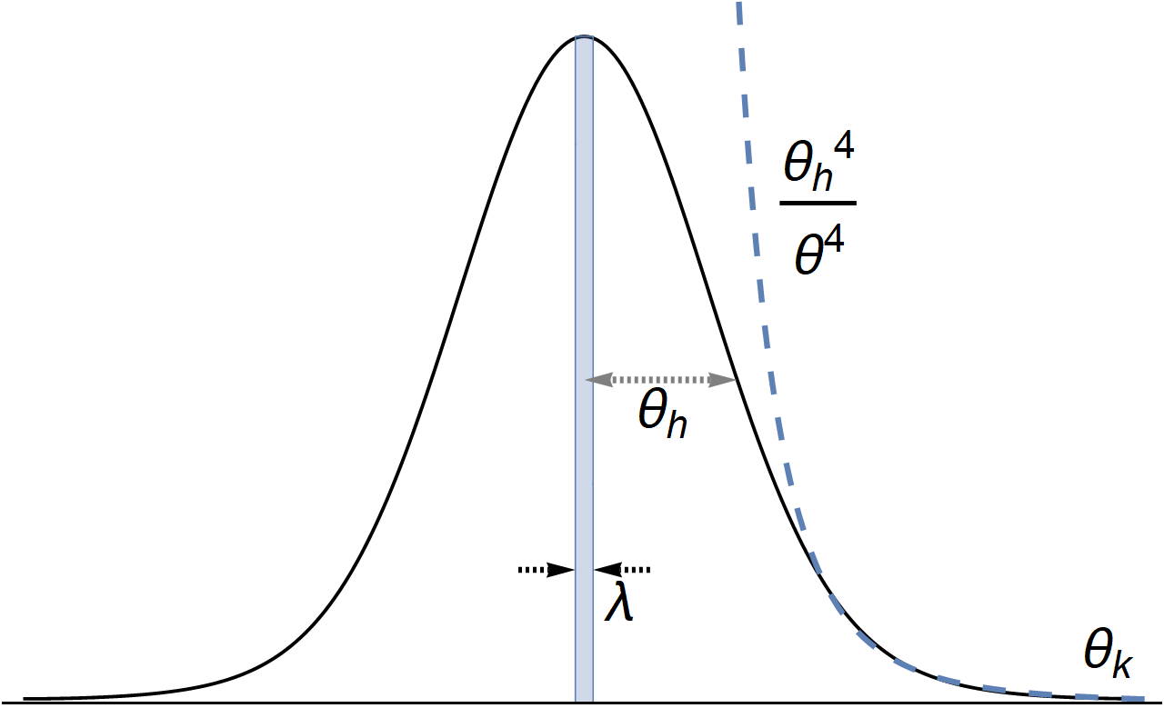

In Fig. 2 we show the result of the numerical solution of the full 2D Eliashberg equation (4). We see that for the full dynamical problem both the width of the interaction, and the width of the gap, are finite at a QCP. This is in contrast to a FL analysis [29], where both vanish as respectively, at a QCP.
wave vs wave pairing symmetry
To obtain the global structure of the gap function and determine the splitting of onset temperatures for wave vs wave pairing, we need to take into account variations of the gap function over large regions of the FS, . Naively, we expect and wave splitting to be determined by whether the nematic attraction prefers a nodal -wave structure or non-nodal wave structure. However, it turns out that the condensation energy from wave nodes is of order , and is much smaller than the actual energy difference which is of order . Instead, the splitting originates from the difference in the interactions between hot regions. To show this, we again reduce the 2D integral equation (4) to the effective 1D equation on , as in Eq. (9), but now do not expand the r.h.s. in small and . The full effective 1D equation differs from (9), and this difference can be modeled by introducing eigenvalues , different for wave and wave pairing. Setting , we then obtain
| (12) |
One can verify that larger eigenvalue corresponds to larger . Our goal is to find .
The leading contribution to the r.h.s. of (12) comes from . This leading term, however, does not differentiate between wave and wave pairings. The one which differentiates between the two comes from the range of order near . This contribution is of order (the additional is due to in the region ). Accordingly, the splitting between wave and wave couplings is
| (13) |
The eigenvalue splitting gives rise to the splitting between and : (i.e., ). One can verify that the higher eigenvalue is , as one expects considering that the interaction is purely attractive. We also verified Eq. (13) by numerically solving Eq. (4) [44].

Eqs. (8) and (13) portray the interplay between long- and short- scales near a QCP. The divergence of static fluctuations near the QCP is cut off by the boson dynamics, setting the IR scale of momentum transfer . Interactions at this scale provide the largest contribution, of order , to in both wave and wave channels. The degeneracy between in the two channels is lifted by the much weaker interaction at large momentum transfer of , and has additional smallness in . Note that although , the the effective 1D equation (12), from which we extracted , neglects self-energies at large angles, so we don’t need to compute self-energies to order .
Summary.
In this communication we studied strong coupling theory of SC in a metal near a QCP towards nematic order. We used fermion-boson model, and treated the ratio of effective boson-fermion coupling and the Fermi energy as a small parameter . We solved the linearized Eliashberg equation and verified that is finite at a QCP and is of order for both wave and wave pairing. The two are not degenerate and is larger than , but the difference is much smaller than each of these temperatures. We also analyzed angular variation of the superconducting order parameter along the FS. We showed that is the largest in hot regions on the FS, whose width . Within a hot region (at ), the order parameter is approximately a constant. Outside, it drops as and becomes smaller by a factor . This behavior holds for both wave and wave order parameters. The two become different only at .
We end with a word of caution. In this work we considered which monotonically decreases between hot and lukewarm regions and does not change sign along the arc . There exist other wave and wave solutions of Eq. (4), which change sign times. These additional solutions emerge at smaller and do not affect , , and the structure of near in each channel. Still, if for these additional solutions of the linearized equation is small compared to only by some power of , we expect that the form of near will be quite different from that near .
Acknowledgements.
We thank E. Berg, R. Fernandes, S. Kivelson, M. N. Gastiasoro, S. Lederer and Y. Schattner for stimulating discussions. This work was supported by the NSF DMR-1523036. We acknowledge the Minnesota Supercomputing Institute at the University of Minnesota for providing resources that assisted with this work.References
- [1] H. v. Löhneysen, A. Rosch, M. Vojta, and P. Wölfle, Rev. Mod. Phys. 79, 1015 (2007).
- [2] P. Monthoux, D. Pines, and G. G. Lonzarich, Nature 450, 1177 (2007).
- [3] A. Abanov, A. V. Chubukov, and J. Schmalian, Advances in Physics 52, 119 (2003).
- [4] D. J. Scalapino, Rev. Mod. Phys. 84, 1383 (2012).
- [5] S. Sachdev, M. A. Metlitski, and M. Punk, Journal of Physics: Condensed Matter 24, 294205 (2012), and references therein.
- [6] O. Cyr-Choinière, R. Daou, F. Laliberté, C. Collignon, S. Badoux, D. LeBoeuf, J. Chang, B. J. Ramshaw, D. A. Bonn, W. N. Hardy, R. Liang, J.-Q. Yan, J.-G. Cheng, J.-S. Zhou, J. B. Goodenough, S. Pyon, T. Takayama, H. Takagi, N. Doiron-Leyraud, and L. Taillefer, Phys. Rev. B 97, 064502 (2018).
- [7] L. Taillefer, Annu. Rev. Condens. Matter Phys. 1, 51 (2010).
- [8] T. Shibauchi, A. Carrington, and Y. Matsuda, Annu. Rev. Condens. Matter Phys. 5, 113 (2014).
- [9] A. Coldea and M. Watson, ArXiv:1706.00338 .
- [10] R. M. Fernandes, A. V. Chubukov, and J. Schmalian, Nat Phys 10, 97 (2014).
- [11] F. Wang, S. A. Kivelson, and D.-H. Lee, Nat Phys 11, 959 (2015).
- [12] Y. Wang and A. Chubukov, Phys. Rev. B 90, 035149 (2014).
- [13] A. Abanov, A. V. Chubukov, and A. M. Finkel’stein, EPL (Europhysics Letters) 54, 488 (2001).
- [14] Y. Wang, A. Abanov, B. L. Altshuler, E. A. Yuzbashyan, and A. V. Chubukov, Phys. Rev. Lett. 117, 157001 (2016).
- [15] S. Raghu, G. Torroba, and H. Wang, Phys. Rev. B 92, 205104 (2015).
- [16] B. L. Altshuler, L. B. Ioffe, and A. J. Millis, Phys. Rev. B 50, 14048 (1994).
- [17] M. A. Metlitski and S. Sachdev, Phys. Rev. B 82, 075127 (2010a).
- [18] M. A. Metlitski and S. Sachdev, Phys. Rev. B 82, 075128 (2010b).
- [19] M. A. Metlitski and S. Sachdev, New Journal of Physics 12, 105007 (2010c).
- [20] S. Lederer, Y. Schattner, E. Berg, and S. A. Kivelson, Proc Natl Acad Sci USA , (2017).
- [21] S.-S. Lee, Annu. Rev. Condens. Matter Phys. 9, 227 (2018).
- [22] M. A. Metlitski, D. F. Mross, S. Sachdev, and T. Senthil, Phys. Rev. B 91, 115111 (2015).
- [23] N. E. Bonesteel, I. A. McDonald, and C. Nayak, Phys. Rev. Lett. 77, 3009 (1996).
- [24] C. Nayak and F. Wilczek, Nuclear Physics B 430, 534 (1994a).
- [25] C. Nayak and F. Wilczek, Nuclear Physics B 417, 359 (1994b).
- [26] E. Fradkin, S. A. Kivelson, M. J. Lawler, J. P. Eisenstein, and A. P. Mackenzie, Annu. Rev. Condens. Matter Phys. 1, 153 (2010).
- [27] J. Rech, C. Pépin, and A. V. Chubukov, Phys. Rev. B 74, 195126 (2006).
- [28] S.-S. Lee, Phys. Rev. B 80, 165102 (2009).
- [29] S. Lederer, Y. Schattner, E. Berg, and S. A. Kivelson, Phys. Rev. Lett. 114, 097001 (2015).
- [30] Y. Schattner, S. Lederer, S. A. Kivelson, and E. Berg, Phys. Rev. X 6, 031028 (2016).
- [31] R. Mahajan, D. M. Ramirez, S. Kachru, and S. Raghu, Phys. Rev. B 88, 115116 (2013).
- [32] E.-G. Moon and A. Chubukov, Journal of Low Temperature Physics 161, 263 (2010).
- [33] J. A. Hertz, Phys. Rev. B 14, 1165 (1976).
- [34] A. J. Millis, Phys. Rev. B 48, 7183 (1993).
- [35] V. Oganesyan, S. A. Kivelson, and E. Fradkin, Phys. Rev. B 64, 195109 (2001).
- [36] D. L. Maslov and A. V. Chubukov, Phys. Rev. B 81, 045110 (2010).
- [37] A. Klein, S. Lederer, D. Chowdhury, E. Berg, and A. Chubukov, Phys. Rev. B 97, 155115 (2018).
- [38] A. Abanov, A. V. Chubukov, and M. R. Norman, Phys. Rev. B 78, 220507 (2008).
- [39] A. J. Millis, S. Sachdev, and C. M. Varma, Phys. Rev. B 37, 4975 (1988).
- [40] A. Abrikosov and L. Gorkov, Sov. Phys. JETP 8, 1090 (1959).
- [41] A. Abrikosov, L. Gorkov, and I. Dzyaloshinski, Methods of Quantum Field Theory in Statistical Physics, Dover Books on Physics Series (Dover Publications, 1975).
- [42] The numerical factor in Eq. (8) is somewhat different from that in references 11, 43. This is a consequence of the fact that we used the expression for the fermionic self-energy, Eq. (3). A more accurate calculation, incorporating the self-energy at , yields .
- [43] A. V. C. Yiming Wu, Artem Abanov, In preparation (2018).
- [44] “See supplemental material for detailed derivations.” .
Supplementary material
Our supplemenary material has two parts. The first part gives a more detailed derivation of our results on angular variation of the gap function in both hot and lukewarm regions, and on the resulting splitting of critical temperatures between wave wave modes, Eq. (13). The second part discusses the numerical methods used to determine the critical temperature at the QCP, Eq. (8), and to verify our analytic results.
Angular variation of
In the main part of the paper, we noted that the critical temperature is, to first approximation, determined by the local, frequency dependent, gap equation (6). In order to determine the angular behavior, we approximated the full gap equation (4) by an effective one dimensional integral equation where we replaced the frequency terms in the gap equation by their typical value , and summed over the Matsubara frequencies. The result is Eq. (9) which we reproduce here for clarity,
| (14) |
Eq. (14) neglects several angular terms, namely the angular dependency of the fermionic and bosonic self-energies, see Eqs. (2), (3). We have verified that neglecting these terms doesn’t affect the final result. Eq. (14) has been the property that if we neglect the dependence of and on , it is fulfilled trivially.
To determine the width of the hot region gap we assume that is a function of a single scaling parameter , and analyze it for . The r.h.s. of Eq. (14) simplifies to,
| (15) |
where , but . The first term is the local contribution from , and the second term is the induced gap from the nearby hot region at . It is easy to see that for
| (16) |
we obtain a dimensionless equation (for ),
| (17) |
with a solution,
| (18) |
where is a constant of order one. Our results are equivalent to Eqs. (10),(11). Eq. (18) also demonstrates that near the lukewarm regions ,
| (19) |
In order to obtain the transition temperatures for wave and wave gaps, we again reduce Eq. (4) to an effective 1D equation. We account for the expected temperature differences by introducing different eigenvalues for wave and wave solutions , i.e.,
| (20) |
We assume and then verify that , and expand the ’s near , to obtain,
| (21) |
where is the solution, Eq. (8), of the local gap equation (6). Then we have
| (22) |
In order to evaluate we again account for the two contributions from the r.h.s. of Eq. (18), one coming from the local contribution , and the other coming from far regions, . The local contribution is larger, but doesn’t differentiate between wave and wave, which will be determined by the nonlocal contribution. If we consider the behavior at a hot region, say , then the nonlocal contribution will come mostly from the hot regions at . Therefore we have,
| (23) |
where in the integration we shifted . In the second line, one in the last term on the right comes from width of the hot region, and another comes from expanding the form-factor, . is a constant of order one. Eq. (23) implies a splitting , which is second order in . Such splitting is much smaller than what we would naively expect, namely a difference of order . We therefore need to verify that there is no other contribution that is equivalent or larger. To this end we re-iterate Eq. (18), and obtain for ,
| (24) |
Here are constants of order one. The final term comes from one of two contributions: (a) but , or vice versa. This is a contribution from the lukewarm region. (b) , but . This is a contribution from the hot regions. Regardless of origin, the final contribution is clearly smaller than the second term, and so, going back to Eq. (22), we find that the split in scales with . Eq. (22) is equivalent to Eq. (13) in the main text.
Numerical methods
We performed numerical analysis of the two gap equations we studied in the main text: both the full 2D Eliashberg equation, Eq. (4), and the local gap equation, Eq. (6). All of our solutions were obtained in MATLAB 2017.
We solved the local gap equation by numerically finding the largest eigenvalue of the operator on the r.h.s. of Eq. (6). We solved for using an increasing series of Matsubara frequencies, and then performed finite-size scaling. The result is shown in Fig. 4 and was reported in Eq. (8) of the main text.

We solved the full 2D Eliashberg gap equation for a variety of of system sizes in both angle discretization and Matsubara frequencies, , , and a variety of couplings, . All computations were performed using the resources of the Minnesota Supercomputing Institute (MSI). We confirmed numerically the calculated scaling of the hot region width and decay, Eqs. (10), (11). We also confirmed that the eigenvalue splitting between wave and wave solutions of the full equation followed the same scaling as the one we found from the 1D equation, Eq. (13). We also confirmed the expected height of the gap in the lukewarm region, Eq. (19).