Rolling and no-slip bouncing in cylinders
Abstract
Abstract
The purpose of this paper is to compare a classical non-holonomic system—a sphere rolling against the inner surface of a vertical cylinder under gravity—and a class of discrete dynamical systems known as no-slip billiards in similar configurations. A well-known notable feature of the non-holonomic system is that the rolling sphere does not fall; its height function is bounded and oscillates harmonically up and down. The central issue of the present work is whether similar bounded behavior can be observed in the no-slip billiard counterpart. Our main results are as follows: for circular cylinders in dimension , the no-slip billiard has the bounded orbits property, and very closely approximates rolling motion, for a class of initial conditions which we call transversal rolling impact. When this condition does not hold, trajectories undergo vertical oscillations superimposed to an overall downward acceleration. Considering cylinders with different cross-section shapes, we show that no-slip billiards between two parallel hyperplanes in Euclidean space of arbitrary dimension are always bounded even under a constant force parallel to the plates; for general cylinders, when the orbit of the transverse system (a concept that depends on a factorization of the motion into transversal and longitudinal components) has period two—a very common occurrence in planar no-slip billiards—the motion in the longitudinal direction, under no forces, is generically not bounded. This is shown using a formula for a longitudinal linear drift that we prove in arbitrary dimensions. While the systems for which we can prove the existence of bounded orbits have relatively simple transverse dynamics, we also briefly explore numerically a no-slip billiard system, namely the stadium cylinder billiard, that can exhibit chaotic transversal dynamics.
1 Introduction
A classical example of a non-holonomic mechanical system consists of a ball that rolls against the inner side of a vertical cylinder with enough speed so as not to lose contact with the surface. We imagine that the surface of the ball is ideally rough, or rubbery, so that a kind of conservative static friction causes it to roll without slipping. Contrary to common intuition, the ball does not fall to the ground, but oscillates harmonically up and down. This ideal behavior is approximately reproduced in lab experiments; see, for example, [9]. (For a study of this system in the context of the theory of nonholonomic systems see also [2] and [13]. We give below a fairly complete description of it in a form that will serve our present needs.)
Rather than rolling, we imagine that the idealized ball bounces off the cylinder’s inner wall in a kind of grazing motion, but still under the same kind of conservative static friction constraint that couples the linear and rotational components of the motion. Would the ball still defy gravity, so to speak, as in the rolling process?
This question introduces a number of issues. First, how should we define such a discrete system in a way that is reasonably well-motivated, starting from general physical principles such as energy conservation and time reversibility? A good candidate has been studied before under the name of no-slip billiard systems. For some early papers, see [8, 3, 16]. See also [10, 12], as an example of how no-slip collision models are used in situations where exchange of linear and angular momentum of particles is desired. Recently, the authors have begun to pursue a more systematic investigation of the dynamics of no-slip billiards; see [5, 6, 7]. Except for [5]—a differential geometric study of rigid collisions in in which no-slip billiards arise in a natural way—we are only aware of studies that are restricted to dimension . Clearly, we need here to consider such systems in dimension (or greater, if one is also interested, as we are, in related problems of a more differential geometric flavor.)
Another issue to consider is whether any particular choice of dynamical system defined by sequences of impacts can be said to serve as a good model for a theory of discrete nonholonomic dynamics. Concretely, does the discrete model exhibit similar properties as the continuous time system, such as having bounded (e.g., not falling to the ground) trajectories; and do grazing trajectories approximate the well-studied rolling motion?
The purpose of this paper is twofold. First, we wish to pursue the problem of existence of bounded trajectories of no-slip billiards in generalized cylinders in dimensions and greater. By a cylinder we mean a domain in that has translation symmetry along an axis. (The -dimensional circular cylinder will have some prominence here, but we also consider other domains.) In dimension , [3] showed that the no-slip billiard motion in an infinite strip is bounded, and in [6, 7] we extended and refined this observation in a way that provides some insight into the dynamics of general polygonal no-slip billiards. As might be expected, the higher dimensional story is more subtle; we describe in this paper some of the new phenomena that arise beyond dimension . Another goal is to make a direct comparison between the rolling and no-slip (bouncing) dynamics. One of our main results here, which is specific to circular cylinders in dimension , is that for a set of initial conditions that we refer to as transversal rolling impact, the billiard motion is indeed bounded. We also show numerically that the discrete system very closely approximates rolling under the just mentioned class of initial conditions. On the other hand, if these conditions are not satisfied, it is observed numerically that the ball will acquire an overall acceleration under an external force.
There are many natural questions that we do not yet pursue in this study. For example, when can the discrete system be said to be integrable? (See [2] for a proof of boundedness of orbits for rolling in -dimensional cylinders of arbitrary cross-section using the existence of integrals of motion; our proof that no-slip billiard motion between parallel hyperplanes in under constant force is bounded also makes used of conserved quantities in a suggestive way.) What can be said about the preservation of the canonical Liouville measure? (We give sufficient conditions for the invariance of this measure in [5], and show that the measure is preserved for no-slip billiards in dimension , but the question is as yet open in higher dimensions. The non-preservation of the Liouville measure is a feature of many non-holonomic mechanical systems.) Moreover, proving that the differential equations for rolling can be obtained as a limit of the discrete equations of the no-slip billiard with short intercollision flights is a natural question that has eluded us so far. Our numerical experiments suggest that a certain transversal rolling impact defect parameter introduced below should play a central role. The focus of the present paper is not on such general issues but is aimed mainly at pointing out interesting phenomena that can be observed when comparing rolling and bouncing motion in such velocity constrained systems, as well as proving results on boundedness of orbits for generalized cylinders that do not have a rolling counterpart.
The rest of the paper is outlined as follows. The next section summarizes the paper’s main observations. Section 3 sets up the geometric notation and background for defining the no-slip collision map. Section 4 gives a self-contained overview of rolling on cylinders with general cross section. Sections 5, 6, and 7 give proofs of the main results. We conclude in Section 8 with some numerical observations and a proposal for future work on no-slip billiards in cylinders whose transverse dynamics exhibit chaotic behavior.
2 Main definitions and results
We begin with a few definitions and, in particular, recall the notion of no-slip billiards. Let denote the ball of radius centered at the origin in . It is given a mass distribution measure having total mass . We assume that the first moment is zero and let be the matrix of second moments per unit mass:
Only mass distributions for which is scalar, , where is the identity matrix in dimension , will be considered here. When is rotationally symmetric and has a continuous density relative to the volume measure, then, expressed in terms of the density as a function of the radial coordinate,
where is the volume of an -dimensional ball of radius . It is convenient to introduce the parameter . For example, and if is constant. It is not difficult to see that, for a general rotationally symmetric mass distribution, and .
Let be an open connected region in . Let be the closure of the set of for which the ball of center and radius is contained in . We assume that is a manifold with corners as defined in [11]. We refer to as the billiard domain and, occasionally, to as the enlarged billiard domain. For regular points of the boundary (that is, a point at which a tangent space is defined) define to be the unit normal vector field pointing towards the interior of . Denote by the Euclidean group of positive isometries of . Its elements will be written as pairs acting on by affine transformations on .
The configuration manifold of a spherical particle of radius with center in is the manifold with corners consisting of all such that . Naturally, a boundary point of is a pair such that .
In this paper we are interested in rolling and bouncing motion in cylinders, by which we will mean the following, unless further geometric assumptions are made:
Definition 1 (Cylinders in ).
A solid cylinder in with axis vector is a domain such that for all and . Here is a unit vector in that defines which direction is up. Writing , we have . The boundary cylinder will be written , where .
As far as the rolling process is concerned, all we will need is the boundary cylinder ; the solid cylinder will be needed for the no-slip billiard systems. For rolling we also assume that is a smooth hypersurface in , whereas for the billiard motion we may allow singular points so long as we consider orbits that avoid them.
From the spherically symmetric mass distribution with second moments matrix , , we define the kinetic energy Riemannian metric on as follows: Let and be vectors tangent to at . Then
| (1) |
It is easily checked that this bilinear form is (the restriction to of) a left-invariant Riemannian metric on .
Observe that if is a differentiable curve in , then its derivative at is given by where and , where is an element of the Lie algebra of the rotation group. The kinetic energy of the moving ball with state at configuration is then written in the norm associated to the Riemannian metric as . Notice that the metric and the kinetic energy function do not depend on .
The boundary of the configuration manifold has a special structure that will be important for our concerns, which we call the no-slip bundle. It is a vector subbundle of the tangent bundle to , denoted , and defined as follows.
Definition 2 (The no-slip bundle).
At each regular point , , describing a boundary configuration of the moving particle system, define
| (2) |
where is the radius of the particle. We call the no-slip space at .
This definition has a clear motivation if we note that the point of contact of the moving particle with the boundary of the extended domain has velocity
Thus a state of the system (that is, a tangent vector at some point of ) at a boundary configuration is in the no-slip bundle if the point of contact of the particle with the boundary of the domain has velocity. (The reader should keep in mind the distinction between the billiard domain and the enlarged domain ; the former contains the center of masses of the particle, and the latter contains the entire ball of radius around those centers in .)
Definition 3 (No-slip rolling).
A particle whose motion is described by a smooth curve is said to undergo (no-slip) rolling if for each . We also say in this case that the particle rolls with no slip on the boundary surface of the (enlarged) billiard domain.
We consider next the dynamical equations describing the motion of a particle of radius , mass , and rotationally symmetric mass distribution with parameter , that rolls with no-slip on the boundary of the enlarged domain . With some innocuous abuse of language we speak of rolling on , the locus of the centers of mass of the moving particle, rather than the hypersurface of contact points. Keeping this in mind, we will avoid when possible referring to .
For the details on non-holonomically constrained systems we suggest [1]. Let be a vector field on which we interpret as a force field. The motion of the unconstrained system is governed by Newton’s equation , where is the Levi-Civita connection for the kinetic energy Riemannian metric (1). The constraint (rolling on the boundary hypersurface ) can be imposed by adding a force field taking values in . This is the force needed to keep in . As , the constraint force does no work.
Definition 4 (Constrained Newton’s equation).
A smooth path satisfies the constrained Newton’s equation with force field and non-holonomic constraint defined by the no-slip bundle if for all and
where lies in .
So far the interior of has not been relevant since in the rolling process the center of the moving particle must remain on the boundary hypersurface . This will change, of course, as we consider next the notion of no-slip bouncing. Before stating the definition, we recall the set-up of no-slip billiard systems. (The reader is referred to [5] for a detailed account of what is briefly skimmed over below, and to [7] for some dynamical results for -dimensional systems.) In a billiard system in , the motion of the particle (of radius and spherically symmetric mass distribution of total mass and distribution parameter ) consists of a sequence of flight segments in the interior of separated by instantaneous collisions with the boundary . The inter-collision flights are described by the unconstrained Newton’s equation , or by geodesic motion if no forces are present. Collisions at a given point are defined by a linear map that sends pre-collision vectors, that is, vectors in to post-collision vectors in , where is the inward pointing unit vector at a boundary point .
The map will be selected based on the following physical assumptions: (1) Collision is energy preserving; this means that is an orthogonal map relative to the Riemannian norm on . (2) It is time reversible, which forces to be a linear involution. (3) The orthogonal component of the pre-collision velocity in the no-slip subspace is not affected by . This third requirement is natural since an (instantaneously) rolling collision, for which the point of contact is stationary, should not cause a change in linear or angular velocities due to an exchange of momentum at impact, except in the direction . In fact, a more careful analysis of the impact event (as in [5]) identifies the orthogonal complement of as the space containing impulse vectors. Ordinary billiard systems are those for which is the identity not only on but also on the subspace of perpendicular to , in which case rotation and translation components of the motion are de-coupled and the rotation part may be ignored. In other words, for standard billiards, the collision maps are specular reflection (in the kinetic energy inner product). This corresponds to a perfectly slippery contact between the moving particle and the boundary of the billiard domain. If instead we wish to model the behavior of a perfectly elastic ball with a perfectly rough (or rubbery) surface, for which angular and linear velocities may be partly exchanged at collision, then we are forced under the other assumptions to require to be the negative of the identity map on the full orthogonal complement of the no-slip subspace (which here includes .) With this in mind we state the following definition.
Definition 5 (No-slip bounce).
A no-slip bounce at is the correspondence sending a pre- to a post-collision velocity at defined by the no-slip collision map . The latter is the orthogonal (relative to the kinetic energy Riemannian metric (1)) linear involution of equal to the identity on and minus the identity on this space’s full orthogonal complement.
Due to the spherical symmetry of the moving particle’s mass distribution and the discrete nature of the billiard process, it is less relevant for no-slip billiard systems that we keep track of the actual rotation matrix . In fact, prior to each collision, we can imagine that the particle is rotated back to a fixed reference orientation in space, keeping linear and angular velocities unaffected. This leads to the notion of reduced phase space at boundary configurations. With , we define
| (3) |
whose elements are triples , . In other words, we may assume that, at each collision, the rotation matrix is the identity and only keep track of the matrix of infinitesimal angular velocities, in addition to the point representing the velocity of the center of mass at . Since will not be involved, we write rather than when viewing it as a map on
We now turn to no-slip billiards on solid cylinders with axis vector . If is a point in , we occasionally write for its projection to the cross-section ; similarly, if is a tangent vector at , its projection to a vector at on the cross-section may be written .
The cross-section domain has its own no-slip billiard system, with a ball of dimension as the moving particle. The latter will also have a spherically symmetric mass distribution (if this is the case for the -dimensional particle) given by the marginal mass distribution after integrating along . In this case the parameter for the -dimensional particle is the same as for the -dimensional one.
For standard billiard systems on a cylinder (for which reflection is specular), it is both clear and unremarkable that trajectories of the -dimensional system should project to trajectories of the billiard system on . This is due to conservation of momentum resulting from the translation symmetry along . For the no-slip billiard, this component of momentum is no longer conserved. Nevertheless this projection property still holds.
Theorem 6.
Let be the reduced phase space of the no-slip billiard system on the solid cylinder domain , and let be the reduced phase space for the associated transverse billiard system. Then trajectories of the no-slip billiard on , possibly with a constant force in the longitudinal direction, project to trajectories of the no-slip billiard map on , where the latter system is given the same mass distribution parameter as the billiard in dimension .

The above theorem only expresses part of a very useful decoupling of the full set of linear and angular velocity components into two that will greatly facilitate the study of the displacement of the particle’s center of mass along the longitudinal direction. (See Proposition 20.) To anticipate what is to come, we note that the Lie algebra of the Euclidean group splits into the Lie algebra of , the group associated with the transversal system, and the orthogonal complement of the latter Lie algebra with respect to the kinetic energy metric. The no-slip collision map will factorize according to this orthogonal decomposition, and our main interest will be on the factor since this is the one that contains the -component of the center of mass velocity. The subspace has dimension ; this means that, so long as we are concerned with the longitudinal motion, we only need to focus on out of velocity components (the latter number being the dimension of ). Therefore, an investigation of the motion of the moving particle naturally splits into a study of the transverse billiard system on and a reduced system containing the component of the motion along .
For -dimensional no-slip billiards in cylinders, this theorem says that the transversal part of the motion reduces to understanding no-slip billiard dynamics in dimension . In the course of this paper we refer to a few results in dimension established in our [7]. In general however the focus of the rest of the paper is on the motion along the axis of translation symmetry set by the axis vector , rather than on the transverse dynamic, and in particular on the question of boundedness of orbits. Note that we will refer to the direction along as the longitudinal direction or the vertical direction, using the terms interchangeably.
We now summarize our main results concerning the question of whether or not trajectories are bounded in the longitudinal direction of the cylinder. As will be seen, the general answer is: sometimes yes, and sometimes no. The following theorem extends the main result of [3] from free motion in -dimensional strips to possibly forced motion in -dimensional regions bounded by parallel hyperplanes. (This domain is a cylinder, according to our general definition.)
Theorem 7.
Consider a domain whose boundary consists of two parallel hyperplanes in , . Then a trajectory of the no-slip billiard system whose initial center of mass velocity is not parallel to the hyperplanes is bounded. Trajectories remain bounded if a constant force is applied to the particle’s center of mass along any direction parallel to those hyperplanes.
Next we ask wether the property of having bounded orbit holds for general cylinders. We show that even in the absence of forces the motion may not be bounded. Typically the height of particle’s center of mass will possess a drift in one direction along the cylinder axis superimposed to an oscillatory part.

Before validating this claim, we observe that, due to Theorem 6, it makes sense to talk about transversely periodic trajectories of the cylindrical billiard. In dimension , transversal period orbits are very ubiquitous and easy to obtain. (See Section 3 of [7].) Figure 2 shows the conditions under which they arise. Observe that, for , the constraint equation on initial conditions for period orbits involves only the projection of the linear velocity to the cross-section plane and of the -component of the angular velocity vector (which is as indicated in Figure 2). In particular, no conditions are imposed on the velocity components that appear in the description of the longitudinal motion.
What follows is a corollary of Theorem 21. (The theorem holds for general cylinders in arbitrary finite dimension.) Referring to Figure 2, we regard and as the tangent and normal vectors at the first collision point and as the pre-collision angular velocity at that point; is as indicated in that figure.
Corollary 8.
A transversal period orbit of a -dimensional general cylinder billiard, under no forces, with initial linear vertical velocity and initial angular velocity vector has a vertical drift
where and are the and components of , and is the height (ie. signed vertical displacement) after collisions. The condition on the orbit for having transversal period does not restrict the values . Thus the motion is generically unbounded in the vertical direction. If the vertical drift is , the motion is bounded.
We wish next to compare the no-slip billiard system in circular cylinders with the rolling process. Let us first review the classical fact about bounded orbits for the rolling motion.
Proposition 9.
Suppose that the cross-section of the -dimensional vertical cylinder is a differentiable simple closed curve and that —the vertical component of the angular velocity vector, a constant of motion—is non-zero. Then trajectories of the rolling motion under a constant force parallel to the axis of the cylinder are bounded.
Implicit in this statement is the assumption that the particle is constrained to remain in contact with the surface.

As an illustration, consider the stadium cylinder whose cross-section, depicted in Figure 3, consists of two circular caps connected by parallel line segments. A glance at the second order equation for the height function in Theorem 19 shows that the ball is essentially in free fall (with acceleration ) while it rolls on the flat parts of the surface. In order to remain bounded, it must rebound upward when it passes over the curved caps. Figure 4 shows a typical height function. In the final section of the paper we will briefly explore numerically the no-slip billiard version of this example. It will be apparent that the question whether (and under which initial conditions) orbits remain bounded is much more challenging when the transverse no-slip billiard system is chaotic.
Let us return to the circular cylinder. Compared to rolling motion, the behavior of a no-slip billiard system inside a cylindrical billiard domain, in the presence of a constant force pulling the particle downward, seems to be more subtle. On the one hand, it is possible, and typical for general cylinders, for the particle to accelerate downward (as one might expect). See Figure 6.

But in dimension and for ordinary circular cylinders, we show that for a class of initial conditions satisfying what we call transversal rolling impact, the particle does not fall: its position along the axis of the cylinder remains bounded.
Prior to stating the definition of rolling impact, observe that if is the pre-collision state at a boundary point , then the velocity of the point of contact of the spherical billiard particle of radius and the boundary of is . We say that the collision satisfies the rolling impact condition if the component of tangent to the boundary of at is zero.
Definition 10 (Transversal rolling impact).
The pre-collision state will be said to satisfy the rolling impact condition if the orthogonal projection of to is zero. If the billiard domain is a cylinder (not necessarily circular) whose axis is parallel to the unit vector , we say that satisfies the transversal rolling impact condition if the orthogonal projection of to is zero.

The above definition of rolling impact is equivalent to the following: at each boundary configuration of the no-slip billiard, an initial state projects to a vector in the no-slip subspace . Here we are referring to the orthogonal projection relative to the kinetic energy inner product on , whereas in Definition 10 it is the ordinary Euclidean inner product that is being invoked. Also notice that transversal rolling impact means that the rolling impact condition holds for the transversal billiard system, which is well-defined due to Theorem 6.

For cylinders in dimension , let denote the unit tangent vector to at , oriented so that form a positive basis. Let be the angular velocity vector. (We recall that is defined by for all .) Then the rolling impact condition is in this case expressed by the equation and the transversal rolling impact condition by
| (4) |
as a simple algebraic manipulation involving the cross-product shows. We take as a measure of the failure in satisfying this condition the quantity and call it the transversal rolling defect (evaluated on the initial velocities).
The following simple observation is essential.
Proposition 11.
Consider a two-dimensional no-slip billiard system in a disc. If the first collision satisfies the rolling impact condition, then all subsequent collisions also do, and the times between consecutive collisions are all equal. Furthermore, the center of mass of the moving particle undergoes specular reflection at each collision.
The main theorem for no-slip billiards in circular cylinders is now the following.
Theorem 12.
Consider a no-slip billiard system in a circular cylinder in whose moving particle is subject to a constant force directed along the axis of the cylinder. If the first collision satisfies the transversal rolling impact condition and the first flight segment does not go through the axis of the cylinder, then the particle’s trajectory is bounded.
Figure 5 shows that the rolling motion and the billiard motion consisting of a sequence of short no-slip bounces, under the assumption that the initial velocities satisfy the transversal rolling impact condition are, in fact, very close.
One may be inclined to think that the equations for the billiard motion are a simple-minded discretization of the differential equation for the rolling motion, or that the latter is a straightforward limit of the former, but this seems not to be the case. It is essential here to bear in mind the phenomenon illustrated in Figure 7, which shows that if the transversal rolling defect is not , then in the continuous limit one obtains a kind of motion that appears to be smooth but is very different from that of solutions of the rolling differential equation. The small scale zig-zag motion shown more clearly in Figure 8, which has a close-up of segments of trajectories highlighting the effect of introducing a small transversal rolling defect, suggests a potential difficulty to overcome. It would be most interesting to find a limit differential equation containing this rolling defect as an equation parameter, and the rolling equations as a special case when the parameter is . Such an equation would, hopefully, suggest a possible physical interpretation of this key parameter. We leave this as a problem to be addressed in a future work.

The proofs of the above theorems and propositions, and of some of the more general facts to be stated shortly that are not restricted to dimension , will be given in the subsequent sections. Although our more complete observations pertain to dimensional domains, we have chosen to state and prove our results, whenever we can, in arbitrary dimensions. We believe that this subject touches on a number of questions of geometric/dynamical interest, for example, concerning a possible theory of discrete non-holonomic systems, for which it would be too restrictive to remain in dimension . Partly for this reason, but also for the sake of completeness, we have also included reasonably detailed proofs of properties of rolling motion, such as the fact that general cylinders in dimension have bounded orbits, even though this is a classical fact. We believe that our more geometric approach, which avoids relying too much on background material from mechanics (like the use of such concepts as Coriolis torque, for example; see [9]) and highlights the central role of the Euclidean group, is worthwhile recording.

3 More definitions and basic facts
There are two Riemannian metrics we need to consider: the one on defined above by (1), and the metric on the hypersurface induced (by restriction) from the Euclidean metric in . Although the context should make it clear which is being referred to at any given moment, for example, when stating that vectors have unit length or are mutually orthogonal, we will always refer to the former as the kinetic energy metric.
We define the cross-product in as the bilinear map taking on values in the Lie algebra of the rotation group, given by
for all If and are unit orthogonal vectors and is the plane linearly spanned by and , then
is a rotation matrix that restricts to the identity transformation on and rotates vectors in by angle , where and are the orthogonal projections to and , respectively. (We also use , possibly with additional sub- or superscripts, for other orthogonal projections to appear in the course of this paper. It will be clear in each case to which projection we are referring.) It is useful to note that
| (5) |
where denotes transpose. If moreover is an matrix then
| (6) |
Notice that, if ,
where is the ordinary cross-product of vector algebra.
The kinetic energy Riemannian metric (1) is a product metric on . The trace part is a bi-invariant metric on the rotation group. It is a standard and easy to prove fact that the Levi-Civita connection on associated to this metric satisfies
for any pair of left-invariant vector fields. The following proposition is also a standard fact about bi-invariant metrics.
Proposition 13.
Let be a smooth path in where the rotation group is given the above bi-invariant trace metric. Define , where indicates derivative in of the matrix-valued function. Then
In particular, is a geodesic iff is constant and
We often find it convenient to express tangent vectors to the Euclidean group at a point in the form , where and . In this form, the vector is obtained by a right-translation from the identity to of an element of the Lie algebra of . The reader should be attentive to the distinction between and . The latter arises when we wish to think of as an infinitesimal rotation expressed in the so-called body frame; on the other hand, when writing a tangent vector as , one has the following interpretation: a material point which in configuration is at , will have velocity at equal to In particular, and are, respectively, the position and the velocity of the center of mass of the ball in the state .
If is a smooth curve in and is now defined by , then by Proposition 13
and the last term simplifies to Thus we immediately have the following remark:
Proposition 14.
For a smooth curve in , write , where and . Then the acceleration of relative to the Levi-Civita connection of the left-invariant (kinetic energy) metric (1) is
When the focus is on the geometry of the boundary of with the induced metric, and , then is replaced with where is the Levi-Civita connection of the hypersurface and is a unit normal vector to at .
Recall from Definition 2 the no-slip bundle . A simple computation gives the explicit form of its orthogonal complement relative to the kinetic energy metric. Notice that the unit normal vector to pointing into is , where is the mass of the moving particle. Clearly, lies in that orthogonal complement. However, in what follows, it will be convenient to reserve the notation for the orthogonal vectors to contained in . Thus defined, we have
| (7) |
Properties (5) and (6) of the product are useful for verifications of this kind.
We give now a more explicit description of the no-slip collision map on the reduced phase space introduced in Definition 5. For details we refer the reader to [5]. The abbreviations and will be used throughout the rest of the paper for the quantities:
The angle is defined by these relations. When there is no chance of confusion we may simply write . Recall that is the unit inward pointing normal vector to .
Proposition 15 (No-slip collision map, [5]).
For each , the no-slip collision map at is the linear map such that
Finally, let us also recall the following definition.
Definition 16 (Shape operator).
The shape operator of the hypersurface at is the symmetric linear transformation of mapping to , where is the vector field along of normal vectors and is being used here for the ordinary directional differentiation of -valued functions. (Elsewhere in the paper we also use for the Levi-Civita connection on relative to t he metric induced by the ordinary dot product.) The unit eigenvectors of are called the principal vectors at , and the eigenvalues are the principal curvatures.
4 Rolling motion on cylinders
In this section we review general facts about rolling and give a self-contained discussion of the fact that orbits of the rolling motion on -dimensional cylinders with general cross-section. This is a classical result in non-holonomic dynamics, but we wish briefly to re-derive it here (in the present more geometric setting) so as to see more clearly the parallels with similar bounded motion of the no-slip billiard counterpart. Throughout the section will denote the axis vector of the cylinder, as in Definition 1. Moreover, continues to denote the inward pointing unit normal vector. In order to simplify notation, we will write except when emphasizing the dependence on boundary point.
The rolling particle is subject to a force (a vector field on ), assumed to have zero component and component , where is constant and is interpreted as the acceleration due to gravity. Such an does not directly affect the angular velocities and can be thought to act on the center of mass of the moving particle.
Returning to the constrained Newton’s equation of Definition 4, notice that due to the description of in Equation (7), the constraint force at has the form
where must be determined from the constraint . Using Proposition 14, and writing , where and , we can split Newton’s equation into separate equations for the angular velocity matrix and center of mass velocity :
| (8) |
As before, refers to the Levi-Civita connection on relative to the metric induced by the standard Euclidean metric (dot product) on . The first equation and the definition of imply
| (9) |
while the constraint on (recall the expression for given in (2)) implies
| (10) |
It is not difficult to solve for and obtain an explicit differential equation for . This is done in the next proposition.
Proposition 17.
The path that solves the constrained Newton’s equation for the rolling process is the solution to an initial value problem for the system of the differential equations
Proof.
Let us define for each the linear map
| (11) |
This is an invertible map. To check this claim, let be an orthonormal basis of with . Then a straightforward computation using the basic properties of leads, for , to
| (12) |
Clearly, then, is injective, hence invertible. It may be helpful noting here that is a constant multiple of the trace inner product . If in particular , then
The first equation, for , comes from (10) and the second, for , is immediate from the definition . Thus we only need to justify the third equation. The second equation in (8) gives , and the first gives
In the above we may replace the covariant derivative with the ordinary derivative since the difference is a multiple of , which vanishes after taking the cross product with . Now notice that , where is the shape operator of at . (See Definition 16.) Therefore,
from which we obtain
The desired third equation follows from the definition of . ∎
Since we are particularly concerned with the issue of boundedness of trajectories, we need to obtain information about the function , whose derivative in time is . The next proposition shows how to get a handle on this quantity.
Proposition 18.
Let be the axis vector of the cylinder , the inward pointing unit normal vector field of , , and . Then
holds under the assumption that satisfies the constrained Newton’s equation for the rolling motion of the particle of radius , mass , mass distribution parameter , subject to a constant force . Furthermore,
where , , is an orthonormal basis of consisting of principal vectors, are the respective principal curvatures of , and , . In dimension we have . Letting in this case be the principal curvature in direction , the above equation reduces to
Proof.
By Proposition 17
Now observe that
hence . The first equation of the proposition is now an immediate consequence. The other claims follow easily from definitions. ∎
In dimension there is an orthonormal moving frame consisting of where . The field is parallel (). Furthermore where is a principal curvature, and . When is a circular cylinder of radius (and the extended billiard domain is a circular solid cylinder of radius ), .
Theorem 19.
Let and introduce the angular velocity vector according to the definition Under the conditions and notations of Proposition 18, the following system of equations hold:
and
where is constant in . Notice that , where is the height of the center of mass of the moving particle. In terms of , the above becomes
where and .
Proof.
Observe that
so that
The quantity is constant in . To verify this claim, first observe that, as is collinear to and is collinear to ,
From the third equation in Proposition 17 and Equation (12) we obtain
But Therefore is indeed constant. It remains to understand the term in Observe that and , hence
where the third and fourth equalities made use of Equation (10). Finally, notice that and . We conclude the proof by applying these observations to the last equation in the statement of Proposition 18. ∎
As a simple example, we see that the height of the rolling particle in a -dimensional vertical circular cylinder undergoes simple harmonic oscillations, so long as the constant of motion is non-zero. In particular, the motion is bounded. In fact, suppose the cross-section of is a circle of radius . In this case is constant, so
This has the form where is a positive constant (assuming ). In terms of the variable , the equation takes the form , whose solutions are the bounded functions
The following interesting observation was made in [9]. Let and denote, respectively, the periods of horizontal and vertical oscillation of the rolling ball in the circular vertical cylinder. One easily finds that and . Therefore the ratio of these two periods only depends on the mass distribution parameter : . For example, for the uniform distribution in dimension , so the period ratio in this case is .
We now restate and prove Proposition 9.
Proposition 9.
Suppose that the cross-section of the -dimensional vertical cylinder is a differentiable simple closed curve and that the constant of motion —the vertical component of the angular velocity vector—is non-zero. Then trajectories of the rolling motion under a constant force parallel to the axis of the cylinder are bounded.
Proof.
Let denote, as before, the height of the center of mass of the rolling particle, and introduce and the component of the angular velocity vector . According to Theorem 19, the function can be obtained by solving an initial value problem for the system
where are constants involving the parameters , , and , and are positive. The principal curvature is a periodic function of which is known in advance since it only depends on the point of contact at time along the cross-sectional boundary curve, and we know which point that is from the initial condition and the constant value of . (That boundary point moves at a constant rate .) A simple rescaling of the variables gives the system
where is a constant multiple of and is a periodic function of whose period we may assume without loss of generality to be . Introducing the complex variable , we previous system reduces to For simplicity, let us assume initial conditions. Then the differential equation for has solution
where satisfies . Standard integral manipulations give
for all integers and . The goal is to establish that the real part of , which equals , is a bounded function. Let us verify this fact for , an integer. Another straightforward manipulation of integrals leads to
| (13) |
where and . But
One then notices that the real part of the term in braces in equation (13) must be zero. ∎
5 No-slip billiards in general cylinders
We now prove Theorem 6, reproduced below.
Theorem 6.
Let be the reduced phase space of the no-slip billiard system on the solid cylinder domain , and let be the reduced phase space for the associated transverse billiard system. Then trajectories of the no-slip billiard on , possibly with a constant force in the longitudinal direction, project to trajectories of the no-slip billiard map on , where the latter system is given the same mass distribution parameter as the billiard in dimension .
Proof.
Given a vector space , it makes sense to write the Lie algebra of the special Euclidean group on , as a vector space, in the form where corresponds to infinitesimal translations and is the space spanned by elements , for all . In this notation we have, for ,
and this direct sum decomposition is orthogonal with respect to the inner product on given above in Equation 1. Also observe that the map (Proposition 15), at each on the boundary of , respects the decomposition
since for all for which we have and
| (14) |
Here we are writing , for and , on the reduced phase space . Letting be the no-slip reflection map at of the system on , and writing for the orthogonal projection from to , it follows that
(As already noted, we use the symbol to denote the orthogonal projection on various subspaces of ; the context will make it clear which subspace one is referring to at any given moment.) From these observations we conclude that the natural projection from to the reduced phase space of the transverse billiard system commutes with the respective no-slip billiard maps. ∎
The following notation will be used in our study of the longitudinal motion of no-slip billiards in general cylinders with axis vector . Let denote, respectively, the pre- and post-collision states at the th collision, , for a given trajectory of the no-slip system in ; we write for the inward pointing normal vector to the boundary of at ; the time interval between consecutive collisions, from the th to the st collision, will be denoted ; we further introduce the velocity components and , and the longitudinal projection . Define the following elements of :
The special notation is used here for the first standard basis vector of in order to emphasize that we are dealing with a velocity space mixing linear and angular components, and not the ambient of the billiard domain. Set , , let be the orthogonal projection to , and define
Simple algebraic manipulation using the basic properties of and Proposition 15 gives that maps pre- to post-collision velocity components in the mixed velocity space . Thus , where . Over the intercollision flight, the change in these mixed velocity components is: since and (recall that does not change between collisions). Therefore,
Proposition 20.
With the notation just introduced, the sequence of displacements along the cylinder’s axis satisfies
with initial conditions and .
Proof.
This is a simple consequence of the general form of given in Proposition 15, the above definitions, and the elementary properties of . ∎
Observe that , like , is an orthogonal involution. It has eigenvalues with multiplicity and with multiplicity . In fact we have for all
We turn our attention now to the longitudinal motion when the no-slip billiard orbit is transversely periodic of period . We wish to find an expression for the longitudinal drift in the absence of forces. This is provided by the following theorem.
Theorem 21.
For an orbit with transversal period , define , , and the row vector . Then . Denote by the orthogonal projection onto the eigenspace of for the eigenvalue . Then
where the are bounded terms of an oscillatory character that can be obtained explicitly if desired. Consequently,
In particular, if is not in the spectrum of (which may be the case in even dimensions), the system has bounded orbits. On the other hand, if is not orthogonal to the eigenspace for associated to eigenvalue , then generically in the initial conditions orbits are not bounded. In the above formulas, the constant intercollision time has been set to .
Proof.
For transversal period orbits, one has only to consider two values for , and consequently only two values for and a single value . From we obtain . Setting and without loss of generality, we have
Here we are setting by convention to be the identity transformation. For concreteness, let us assume that is odd: . Then, letting and gives
Notice that
The summation on the right-hand side of the above equation must be bounded. In fact, further decomposing into or blocks (the latter associated to eigenvalue if it is present in the spectrum of ), we end up with sums of a sequence of vectors generated by iterating a non-trivial rotation in dimension or . In particular, it follows that if is not an eigenvalue of (in even dimension) then trajectories having transversal period are necessarily bounded. To conclude, we note that . ∎

From the above theorem we can now derive the claim made earlier that unbounded orbits actually exist, say in dimension , and obtain the explicit formula for the longitudinal drift shown in Corollary 8. This requires that we obtain the explicit form of the rotation matrix and find its spectral decomposition. This is an entirely straightforward but somewhat tedious computation, whose details we omit.
Let us introduce the angle (see Figure 2) and write . Recall that and are reserved for the cosine and sine of the special angle determined by the mass distribution parameter . Also consider the normal and tangent vectors and at the two contact points, as indicated in Figure 9. Then assumes the following form
Now observe that
is a unit length eigenvector for the eigenvalue of . Then an application of the limit formula for the vertical drift from Theorem 21 gives the formula of Corollary 8. Notice that in Theorem 21 is in this case the rank- projection on the subspace spanned by .
6 Forced billiard motion in a circular cylinder
In this section we restrict attention to circular cylinders in dimension . The main goal is the prove Theorem 12, restated below after a couple of propositions.
Proposition 22.
If the pre-collision state of a general (not necessarily a cylinder) no-slip billiard system satisfies the rolling impact condition, then the post-collision state is given by
In words, the center of mass velocity of the moving particle is reflected specularly and the angular velocity matrix remains the same.
Proof.
From the definition of the no-slip collision map , the rolling impact condition , and the relation we obtain
and
as claimed. ∎
Next we restate and prove Proposition 11, which gives a broader context to a property observed in [6].
Proposition 11.
Consider a two-dimensional no-slip billiard system in a disc. If the first collision satisfies the rolling impact condition, then all subsequent collisions also do, and the times between consecutive collisions are all equal. Furthermore, the center of mass of the moving particle undergoes specular reflection at each collision.
Proof.
Let and be consecutive collision points on the boundary of . Let denote pre-collision linear and angular velocities at and the post-collision velocities at . Notice that the latter are also the pre-collision velocities at . Suppose that the rolling impact condition holds at . Then as , we have
where the last equality is due to the post-collision velocity at being the specular reflection of . Therefore the rolling impact condition also holds at . That intercollision times are all equation is a consequence of Proposition 22. ∎
Theorem 12.
Consider a no-slip billiard system in a circular cylinder in whose moving particle is subject to a constant force directed along the axis of the cylinder. If the first collision satisfies the transversal rolling impact condition and the first flight segment does not go through the axis of the cylinder, then the particle’s trajectory is bounded.
Proof.
Reviewing some notation, is here the cylinder of radius along so that is the cylinder of radius along . A trajectory of the billiard system gives a sequence of post-collision states , , and for this trajectory we have the unit normal vectors to where , the tangent vectors to , the intercollision times between the th and st collisions, the longitudinal component of the center of mass velocities , the transversal angular velocity vectors , the position of the center of the moving particle along the cylinder’s axis, and . The stating point of the proof are the equations (and notations) recorded in Proposition 20. We specialize them to this situation by noting that the projection appearing in the lower-right block of the matrix may be written here as . Thus
The are vectors in and the are matrices. Further, the are orthogonal matrices of determinant , as is easily checked. With , then by Proposition 20,
| (15) |
Let be the initial position of the particle’s center of mass, its initial velocity, and the cross-sectional projection. We define as the angle between and , as in Figure 10, and assume that .
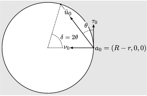
We also assume without further notice that the transversal rolling impact condition holds. The free-flight times are all equal by Proposition 11; the common value is
and for , where . Observe that small values of correspond to near grazing trajectories.
Define the block diagonal matrix . A simple matrix multiplication shows that and
where, we recall, and are here the cosine and sine of the angle . In terms of mass distribution parameter , and . All this notation in place, we now have
| (16) |
We wish to show that the sequence of obtained by iterating these relations is bounded. From Equation (16) we obtain
| (17) |
and
| (18) |
Define . We also obtain from Equation (16), for ,
| (19) |
Equation (18) yields
It is now necessary to better understand . This matrix is the product of two orthogonal matrices, hence orthogonal, with determinant . It has the explicit form
Under the assumption , . Consider the orthonormal basis of defined by the vectors:
Then is an eigenvector of associated to the eigenvalue and the restriction of to is a planar rotation. Relative to the basis , this restriction has matrix form where and Explicitly,
Let and denote, respectively, the orthogonal projections from to the line and the plane , and write for the restriction of to . Notice that cannot be the identity (the equation implies , which is not the case). As is a planar rotation, is nonsingular and
| (22) | ||||
Notice that is bounded. Next, consider the expression
Then
| (23) |
where denotes the floor function. We claim that
| (24) |
This can be shown to hold as follows. Let denote a complex variable. Then
Identifying with and with multiplication by some gives the claimed identity. Consequently,
| (25) | ||||
The third term on the right-hand side of Equation (25) is bounded. The first term can be evaluated by noting that
Concerning the second term, first observe that
so that
Since the rotation group in dimension is commutative, the number does not depend on the unit vector . Therefore
For concreteness, let us assume odd; the case when is even will differ only by a bounded term. For odd we obtain
| (26) |
Returning now to Equation (17), and using the results so far contained in Equations (21), (22) and (26) we notice that the unbounded terms cancel out and we are left with
which is bonded. This concludes the proof. ∎
7 Forced motion between parallel planes
Here we consider the billiard domain bounded by two infinite parallel affine codimension- subspaces of . Let denote the inward-pointing unit normal vector to one of the planes, so that is the (inward pointing) normal vector for the other plane. Let be a unit vector perpendicular to . We suppose that the billiard particle is subject to a constant force and wish to study the motion of the particle’s center of mass along a direction . The next theorem, which is a restatement of Theorem 7, asserts that this motion is bounded.
Theorem 7.
Consider a domain whose boundary consists of two parallel hyperplanes in , . Then a trajectory of the no-slip billiard system whose initial center of mass velocity is not parallel to the hyperplanes is bounded. Trajectories remain bounded if a constant force is applied to the particle’s center of mass along any direction parallel to those hyperplanes.
Proof.
This theorem admits a proof very similar to that of Theorem 12, but we give instead a more conceptual proof that makes use of a certain invariant quantity that we can identify for the two planes system, but whose possible counterpart for the circular cylinder is not yet apparent to us.
For any given set of initial conditions, the time between two consecutive collisions is constant throughout the orbit; we denote it by . As before, we let denote the position of the center of mass of the moving particle at the th collision with the boundary of the billiard domain. Due to Theorem 6, the proof may be approached by induction: we can focus on the motion in the plane spanned by and and then argue by induction that trajectories are bounded for the transverse billiard system on .
Set , where and is the post-collision angular velocity matrix at step . Let the constant force be , where is the particle’s mass. The component of in the direction is and the component of the post-collision velocity in the direction is . Then
It is also useful to introduce the angular displacement
The following observation is key: For the billiard domain between two parallel planes, possibly with a transverse force, the ratio of angular to linear displacements remains constant after an even number of collisions. In particular,
| (27) |
The proof of this claim is a calculation. For any even we may reindex to , and
As before, we write and Due to Proposition 20,
Notice that and . Thus we arrive at
If is odd, a similar calculation yields . It follows from this observation that
| (28) |
We will refer to these lines as the lines of contact. The constraint obtained from the existence of the lines of contact, combined with conservation of energy, bounds the orbits, as we now show.
Notice that the kinetic energy, expressed in terms of and the rescaled angular velocity is . Up to a common additive constant, the total energy at step is
where is the constant value of the total energy. Setting , we have
| (29) |
The linear relations given by Equations (28) yield
where the constant only depends on initial values. The above energy equation gives
Inserting the previous two equations into (29),
This is the equation of an ellipse in the -plane. A similar ellipse is the locus of . Therefore we can conclude that the sequence is bounded. ∎
8 Final comments: chaotic billiards
The examples of no-slip billiards considered so far in this paper (transversal period , parallel hyperplanes, circular cylinder) all share the property that the associated transversal systems have simple and well-understood behavior. If we were to look for a notion of completely integrable no-slip billiard systems, these would be models to have in mind.
We wish now to consider a numerical example whose transversal dynamics can exhibit chaotic behavior, for which the problem of bounded orbits is likely to be much more challenging.
Let us revisit the stadium cylinder, whose cross section was shown in Figure 3. The rolling motion, as already noted, is bounded, and has a typical quasi-periodic character (see Figure 4), but the corresponding no-slip billiard behaves much differently. Here we focus on a transition from simple bounded motion to a more chaotic regime at a natural bifurcation point (see Figure 11) as an illustration of how different these two types of dynamics (namely, rolling motion versus no-slip billiards) can be. To better appreciate the changes to orbits due to changes in initial conditions, it is useful to resort to a visualization device that we have called in [7] a velocity phase portrait. We give here a brief review of this simple, but helpful, tool.

For no-slip billiards in dimension , the associated transverse billiard system has a -dimensional reduced phase space . (See the definition above in (3).) This space is the product of a -dimensional manifold—the boundary of the planar billiard domain—and a hemisphere in representing the components of linear and angular velocities relevant to the transversal dynamics.
To make sense of this latter part, notice that the two components of the center of mass velocity and the single angular velocity of the planar billiard contribute two degrees of freedom due to conservation of kinetic energy. (The constant force in the vertical direction does not affect the transversal motion due to Theorem 6.) Vectors in this hemisphere are most conveniently expressed in the moving frame defined by the unit tangent vector to the boundary of the planar billiard domain at a given point , the unit inward pointing normal vector at the same point, and a third unit vector perpendicular to the first two representing a unit of angular velocity of the rotating disc (rescaled by a factor that turns the kinetic energy into a multiple of the ordinary Euclidean square norm in ). Using this moving frame, at each is identified with , and each hemisphere with the points of the unit sphere having positive last coordinate. We further project this upper-hemisphere to the unit disc in . In this way we have a bijection between points in the unit disc and (linear-angular) -velocities at each boundary point of the planar billiard domain.

Three transversal orbit segments for the no-slip stadium-cylinder billiard are shown in Figure 11. In each, the particle begins at the bottom flat side with linear velocity pointing up, and a small angular velocity that causes it to reflect rightward upon first collision. All the other velocity components are set to . When the angular velocity is sufficiently small, orbits are confined to the flat parts of the boundary and thus exhibit the bounded motion established in Theorem 7.
As the angular velocity increases, orbits eventually reach the curved parts, and soon transition to a chaotic regime in which a much larger region of the billiard phase space is explored, as suggested by the rightmost diagram of Figure 11. Figure 12 shows what happens during that transition using the velocity phase portrait. The regular motion restricted to the flat sides of the boundary has the property that the linear-angular -velocity vector rotates in a simple fashion, forming a small circle around the north pole of . As the trajectory barely crosses into the curved parts of the boundary, the possible linear-angular -velocity still remains in a small neighborhood of the north pole, but begins to behave in more interesting ways that are very sensitive to the initial velocities. (See the middle diagram in Figure 12.) As the angular velocity increases further, the linear-angular -velocity spreads throughout the velocity phase portrait as shown by the rightmost diagram in Figure 12.
The height function accordingly changes from simple bounded behavior (when the motion is limited to the flat boundary parts) to the rather more complicated motion over much wider distances shown in Figure 13. This height function is likely not bounded; in fact, the graph in Figure 13 suggests a type of “null-recurrent” behavior as in one-dimensional random walks. Notice the short periods of fast falling and bouncing back up, separated by rough plateaux distributed in a seemingly random fashion. We believe that trying to establish limit theorems for the longitudinal motion of chaotic transverse no-slip billiards in cylinders is a potentially fruitful direction to pursue.

References
- [1] A.M. Bloch, Nonholonomic Mechanics and Control. Springer, Interdisciplinary Applied Mathematics 24, second edition, 2015.
- [2] A.V. Borisov, I.S. Mamaev, A.A. Kilin, The Rolling Motion of a Ball on a Surface. New Integrals and Hierarchy of Dynamics. Regular and Chaotic Dynamics, V. 7, N. 2, 2002.
- [3] D.S. Broomhead, E. Gutkin, The dynamics of billiards with no-slip collisions. Physica D 67 (1993) 188-197.
- [4] N. Chernov, R. Markarian, Chaotic billiards. Mathematical Surveys and Monographs, V. 127, American Mathematical Society, 2006.
- [5] C. Cox, R. Feres, Differential geometry of rigid bodies collisions and non-standard billiards. Discrete and Continuous Dynamical Systems-A, 33 (2016) no. 11, 6065–6099.
- [6] C. Cox and R. Feres, No-slip billiards in dimension two, in Dynamical systems, ergodic theory, and probability: in memory of Kolya Chernov, 91–110, Contemp. Math., 698, Amer. Math. Soc., Providence, RI, 2017.
- [7] C. Cox, R. Feres, H.K. Zhang Stability of periodic orbits in no-slip billiards, to appear in Nonlinearity.
- [8] R.L. Garwin, Kinematics of an Ultraelastic Rough Ball. American Journal of Physics, V. 37, N. 1 January 1969, pages 88-92.
- [9] M. Gualtieri, T. Tokieda, L. Advis-Gaete, B. Carry, E. Reffet, and C. Guthmann, Golfer’s dilemma. Am. J. Phys. 74 (6), June 2006.
- [10] H. Larralde, F. Leyvraz, and C. Mejía-Monasterio, Transport properties of a modified Lorentz gas. J. Stat. Phys. 113, 197-231 (2003).
- [11] J.M. Lee, Introduction to Smooth Manifolds. Graduate Texts in Mathematics 218, Springer, 2003.
- [12] C. Mejía-Monasterio, H. Larralde, and F. Leyvraz, Coupled Normal Heat and Matter Transport in a Simple Model System, Physical Review Letters, V. 86, N. 24, 5417-5420 (2001).
- [13] Yu. I. Neumark, N.A. Fufayev, Dynamics of Nonholonomic Systems, Chap. III, Sec. 2, American Mathematical Society, 1972.
- [14] E.J. Routh, The Advance Part of a Treatise on the Dynamics of a System of Ridid Bodies. Macmillan and Co. 1884; Reprinted from the 6th ed. by Dover, New York, 1955.
- [15] S. Tabachnikov, Billiards, in Panoramas et Synthèses 1, Société Mathématique de France, 1995.
- [16] M. Wojtkowski, The system of two spinning disks in the torus. Physica D 71 (1994) 430-439.