Fusion++: Volumetric Object-Level SLAM

Our map is composed of object instances reconstructed within separate TSDFs, $\mathcal{V}^{o}$, each with a pose defined by a transformation, $\mathbf{T}_{WO}\in SE(3)$, which maps coordinates of a point ${}_{O}\mathbf{p}\in\mathbb{R}^{3}$ from object frame ${\smash{\underrightarrow{\mathcal{F}}_{O}}}$ to coordinates ${}_{W}\mathbf{p}\in\mathbb{R}^{3}$ in World frame ${\smash{\underrightarrow{\mathcal{F}}_{W}}}$. For convenience of notation, homogeneous coordinates are assumed where appropriate (e.g. in transformations), however when explicitly required they are denoted with italics, ${}_{O}{\mathbfit{p}}=[_{O}\mathbf{p}^{\intercal},1]^{\intercal}$. Object instance frames have an origin at the centre of the volume and are sized cubically with an edge-length, $s_{o}$.

Initialisation and resizing: Detections not matched by the procedure described in 3.2 are used to initialize an appropriately sized and positioned instance TSDF. In the $k$^th frame each detection $i$ produces a binary mask $M_{i}^{k}$. We project all the masked image coordinates $\mathbf{u}=(u_{1},u_{2})$ into ${\smash{\underrightarrow{\mathcal{F}}_{W}}}$ using the depth map $D_{k}(\mathbf{u})$,

where $\mathbf{K}$ denotes the $3\times 3$ intrinsic camera matrix, $\tilde{\mathbf{T}}_{WC}^{k}\in SE(3)$ the camera pose estimate.

To robustly size the TSDF in the presence of masks which can occasionally include far-away background surfaces, we do not directly accept the maximum and minimum of this point cloud. Instead we use the $10^{th}$ and $90^{th}$ percentiles of this point cloud (separately for each axis) to define points $\mathbf{p}_{10}$ and $\mathbf{p}_{90}$ respectively, which are used to calculate the volume centre $\mathbf{p}_{o}=\frac{\mathbf{p}_{90}+\mathbf{p}_{10}}{2}$ and volume size $s_{o}=m\lVert(\mathbf{p}_{90}-\mathbf{p}_{10})\rVert_{\infty}$. We use an $m$ of 1.5 to account for erosion and provide additional padding.

Each instance TSDF has an initial fixed resolution along a given axis of $r_{o}$, which we choose to be $64$, and $s_{o}$ is used to calculate the physical size of a voxel $v_{o}=\frac{s_{o}}{r_{o}}$. Therefore, small objects will be reconstructed with fine details and large objects more coarsely, making the map as useful as possible for a given memory footprint.

During operation matched objects may need to be re-sized as new detections include additional areas. To do this, the point cloud of the current mask described above is combined with a similarly eroded point cloud generated from the current TSDF reconstruction. The 3D volume encompassing them both is used to calculate the new volume centre and size as before. To avoid aliasing when re-sizing, we translate the volume centre by discrete multiples of $v_{o}$, and maintain the same $v_{o}$ but increase $r_{o}$, while maintaining an even parity. We also limit the maximum voxel resolution to $128$, by re-initialising the volume as though new if $r_{o}>128$, and limit the maximum object size to be 3m.

Before initialising an instance we require the volume centre to be within 5m of the camera, and a 3D axis-aligned bounding box Intersection over Union (IoU) $<0.5$ with any other volume already in the map. When an object centre is moved, the pose-graph node and associated measurements are also updated as described in Section 3.5.

Integration: For integrating surface measurements from a depth map $D^{k}$ into $\mathcal{V}^{o}$ we take an approach similar to Newcombe et al. [23]¹¹ 1 Code based on https://github.com/GerhardR/kfusion.. $\mathcal{V}^{o}$ stores at each discrete voxel location $\mathbf{v}=(v_{x},v_{y},v_{z})$ both the current normalised truncated signed distance value $S^{o}_{k-1}(\mathbf{v})$ and its associated weight $W^{o}_{k-1}(\mathbf{v})$. If $\mathbf{v}$ projects into a camera frame pixel with a depth value less than the depth measurement plus the truncation distance, $\mu$ (here chosen as $4v_{o}$), then that measurement is fused into the volume in a weighted average fashion. Integration is performed on every frame where the TSDF volume is visible, when 50% of TSDF pixels are validly tracked and the ICP RMSE $<0.03$ (these error metrics are described in more detail in Section 3.3). This is to maintain the reconstruction quality of instances when the camera frame may have drifted.

It is also important to note that the above surface integration is performed throughout the entire volume, regardless of whether it is a masked region or not. To store which voxels correspond to this instance’s ‘foreground’ we also fuse instance mask detections. We view each positive or negative detection as the result of a binomial trial sampled from a latent foreground probability, $p^{o}(\mathbf{v}\in\text{foreground})$. We store foreground $F^{o}_{k-1}(\mathbf{v})$ and not foreground $N^{o}_{k-1}(\mathbf{v})$ detection counts as the $(\alpha,\beta)$ shape parameters in a beta distribution conjugate prior which are initialised with $(1,1)$. When a new detection is matched and the depth measurement is within the truncation distance as above, then we also update the detection counts using the corresponding mask $i$:

with $\boldsymbol{\pi}([x,y,z]^{\intercal})=[x/z,y/z,1]^{\intercal}$ denoting the projection. Finally, to compute whether a voxel is part of the foreground we calculate the expectation,

and use a decision threshold of $E[p^{o}(\mathbf{v})]>0.5$. A visualisation of this is shown in Figure 3.

Raycasting: For tracking, data association, and visualisation we render depth, normals, vertices, RGB, and object indices. Within each object volume $\mathcal{V}^{o}$ we step along the ray with a stepsize of $v^{o}_{s}$ (and $0.5v^{o}_{s}$ when $S_{k}^{o}(\mathbf{v})<0.8$, where $S_{k}^{o}(\mathbf{v})$ is the SDF normalised by $\mu$) and search for the zero-crossing point in $S_{k}^{o}(\mathbf{v})$ where $E[p^{o}(\mathbf{v})]>0.5$ (both values are trilinearly interpolated from neighbouring voxels to smooth the representation). We store the ray length of the nearest of these intersections to avoid searching past that point in another volume.

This alone results in occluding surfaces which are not part of the foreground failing to occlude the ray. If a background TSDF is available, and either no intersection with a foreground object occurs or the intersection is farther than 5cm behind the background TSDF intersection, then the background TSDF ray intersection is used instead.

Existence Probability: To prevent spurious instances from building up over time, we also model the probability of each instance’s existence as $p(o)$ using the Beta distribution, in a manner identical to the foreground mask. For any frame where a predicted instance should be clearly visible (i.e. our raycasted image has more than $50^{2}$ pixels of that instance), then if the instance has been associated to a detection its existence count $e_{o}$ is incremented, and if not its non-existence count, $d_{o}$, is incremented. If $E[p(o)]$ falls below $0.1$, the instance is deleted and the object node with all associated edges are removed from the pose graph (described in Section 3.5).

Semantic Labels: Each TSDF also stores a probability distribution over potential class labels $l_{o}$. Mask R-CNN provides a probability distribution $p(l_{o}|I_{k})$ over the classes given the image, $I_{k}$. We found that the standard multiplicative Bayesian update scheme [15, 20]:

where $Z$ is a normalising constant, often leads to an overly confident class probability distribution, with scores unsuitable for ranking in object detection. Instead here we fuse multiple associated detections by simple averaging:

which produces a more even class probability distribution.

Detections from the Mask R-CNN model [13] for a given frame $k$ contain instances $i$ with a binary mask $M^{i}_{k}$ and class probability distribution $p(l_{i}|I_{k})$. A forward pass takes $\sim$250ms, and although our system is not real-time, this still represents a significant bottleneck and so can be performed in a parallel thread. For GPU memory efficiency, we take only the top 100 detections (scored according to the region proposal network ‘object’ score [27]) and filter for masks not near the image border (within 20 pixels) and where both $\text{max}(p(l_{i}|I_{k}))>0.5$ and $\sum M^{i}_{k}>50^{2}$.

After local tracking (Section 3.3) we use the estimated camera pose and TSDFs already initialised in the map to raycast a binary mask $M^{o}_{k}$ for object instances $o$ in the current view. We map each detection $i$ to a single instance $o$ by calculating the intersection of the two as a proportion of the detection’s area, $a_{\mathrm{detect}}(i,o)=\frac{\sum{M^{o}_{k}\cap M^{i}_{k}}}{\sum{M^{i}_{k}}}$ and assigning the detection to the largest intersection, $\tilde{o}=\operatornamewithlimits{argmax}_{o}a_{\mathrm{detect}}(i,o)$, where $a_{\mathrm{detect}}(i,\tilde{o})>0.2$, otherwise the detection is unassigned. For the integration step, each detection which has been mapped to the same instance is combined by taking the union of the detection masks, and the average of the class probabilities.

We maintain an instance-agnostic coarse background TSDF, $a$, to assist local frame-to-model tracking where/when there are no instances and to handle occlusions. It has a resolution of $256^{3}$ with a voxel size of 2cm. Its initialisation point ${}_{W}\mathbf{p}_{a}=\mathbf{T}^{k}_{WC}[0\quad 0\quad 2.56]^{\intercal}$, is 2.56m along the $z$-axis in the camera frame ${\smash{\underrightarrow{\mathcal{F}}_{C}}}$ to prevent wasted volume as in [37]. The volume is reset when its new initialisation point exits a spherical threshold (1.28m) around the previous volume centre, i.e. $\lVert{}_{W}\mathbf{p}_{a}-\mathbf{T}^{k}_{WC}[0\quad 0\quad 2.56]^{\intercal}\rVert_{2}>1.28$.

We combine the background TSDF with individual instances to raycast (Section 3.1) a ‘layered’ reference frame, denoted $r$, with vertex map, $V_{r}$, normal map, $N_{r}$, and object index map, $X_{r}$, from the previous camera pose, $\mathbf{T}_{WC_{r}}$, with vertices and normals defined in the world frame ${\smash{\underrightarrow{\mathcal{F}}_{W}}}$. The transform to the live frame, denoted $l$, is estimated by aligning the live depth map, after bilateral filtering and projection to a vertex map $V_{l}$ and normal map $N_{l}$ with pixels $\mathbf{u}_{l}$, to the rendered maps with iterative closest point using projective data association and a point-to-plane error, $E_{\mathrm{icp}}(\tilde{\mathbf{T}}_{WC_{l}})$, as described in [23]:

Where $V_{\mathrm{valid}}$ includes any $\mathbf{u}_{l}$ with a corresponding vertex and normal, where there is a corresponding $\mathbf{u}_{r}$ with a valid vertex and normal, and where $N_{r}(\mathbf{u}_{r})\cdot N_{l}(\mathbf{u}_{l})<0.8$ and $\lVert V_{r}(\mathbf{u}_{r})-\tilde{\mathbf{T}}_{WC_{l}}V_{l}(\mathbf{u}_{l})\rVert_{2}<0.1\text{m}$.

We minimize this non-linear least squares problem using the Gauss-Newton algorithm. We linearise $\tilde{\mathbf{T}}_{WC_{l}}$ about the previous estimate with the perturbation, $\boldsymbol{\zeta}$ where $\tilde{\mathbf{T}}_{WC}=\exp(\boldsymbol{\zeta})\bar{\mathbf{T}}_{WC}$. Each row of the $|V_{\mathrm{valid}}|\times 6$ Jacobian, $\mathbf{J}_{\mathrm{icp}}$, corresponds to the residual of a given $\mathbf{u}_{l}\in V_{\mathrm{valid}}$:

The Gauss-Newton iteration can then be implemented as follows (with iteration index $t$):

The $6\times 6$ Hessian approximation, $\mathbf{J}_{\mathrm{icp}}^{\intercal}\mathbf{J}_{\mathrm{icp}}$, and $6\times 1$ error Jacobian, $\mathbf{J}_{\mathrm{icp}}^{\intercal}\mathbf{r}_{\mathrm{icp}}$, are reduced in parallel on the GPU and solved on the CPU using SVD and back substitution. We use a three-level coarse-to-fine pyramid scheme with 5 Gauss-Newton iterations per level.

We perform an additional reduction on the GPU to produce the same system of equations partitioned into pixels, $\mathbf{u}_{l}$, associated to each instance in $X_{r}(\mathbf{u}_{r})$ for pose-graph optimisation and to produce per-instance error metrics. The error metrics are the ICP RMSE, $(|V_{\mathrm{valid}}|^{-1}E_{\mathrm{icp}}(\tilde{\mathbf{T}}_{WC_{l}}))^{\frac{1}{2}}$, and the proportion of validly tracked pixels $\frac{|V_{\mathrm{valid}}|}{|V_{l}|}$. These are used for instance integration and to check whether local tracking is lost. We consider local tracking to be lost when the total ICP RMSE is greater than 0.05m or when at least 10% of the image consists of instance TSDFs and less than half of the pixels are validly tracked, in which case we enter relocalisation mode.

If the system is lost or we reset the coarse TSDF, we perform relocalisation to align the current frame to the current set of instances (if there are any). We found direct dense ICP methods using only the volume reconstructions did not produce accurate results for wide baseline relocalisation as they are sensitive to the initial pose and small objects were often ambiguous without texture constraints. Although alternative dense methods may also prove useful here, we took the approach of using snapshots of sparse BRISK features²² 2 BRISK v.2 with homogeneous Harris scale space corner detection on only the highest image resolution. (with a detection threshold of 10) projected to 3D using the depth map. For a given detection of an object if there is no existing snapshot of the object within $15^{\circ}$ view angle difference, we then add a new snapshot of the object from that pose (see Figure 4).

To re-localise we perform 3D-3D RANSAC against each instance where the dot product with the predicted class distribution is greater than 0.6. We use OpenGV [16] with a minimum of 5 inlier features (within 2cm) to match each object individually. If we find one or more matching objects in the scene, we run a final 3D-3D RANSAC on every point in the scene (from all objects and the background jointly) with a minimum of 50 inlier features (within 5cm) to arrive at a final camera pose. This pose is used to render a new reference image of the map to produce the constraints required for the pose graph optimisation described below.

Our pose-graph formulation is similar to that of [30]. For every frame with a Mask R-CNN detection (including coarse TSDF resets), we add a new camera pose node to our graph. When a new instance, index $o$, is initialised, a corresponding landmark node is added to the graph, defined by the coordinate frame attached to the centre of the object’s volume, $\mathbf{p}_{o}$. The first camera pose node is fixed and defined to be the origin of the world frame, ${\smash{\underrightarrow{\mathcal{F}}_{W}}}$. Each node consists of a full $SE(3)$ transformation from object to World, $\mathbf{T}_{WO}$, or camera to world, $\mathbf{T}_{WC}$, and the measurements are $SE(3)$ relative pose constraints between nodes.

Each relative measurement is derived by employing only the ICP error terms which correspond to the pixels of the specific object $o$ (for object-camera constraints), or the instance-agnostic background $a$ (for camera-camera constraints). To ensure that the measurement coincides with the minimum of the partitioned set’s quadratically approximated error function, an additional Gauss-Newton step is performed using the partitioned $\mathbf{J}^{o}_{\mathrm{icp}}$ (see Section 3.3) to produce ‘virtual’ relative pose measurements $\tilde{\mathbf{T}}^{\prime a}_{C_{k-1}C_{k}}$, between camera nodes, and $\tilde{\mathbf{T}}^{\prime o}_{OC_{k}}$, between camera and landmark objects. The resulting measurement errors for the graph factors are:

For every relative measurement, we approximate the inverse measurement covariance by $\boldsymbol{\Sigma}^{-1}=\mathbf{J}_{\mathrm{icp}}^{o\intercal}\mathbf{J}^{o}_{\mathrm{icp}}$. However, since the way perturbations are modelled differs between the ICP algorithm and the employed pose graph optimiser we need to transform the covariance by considering the relation between the local perturbations. The graph optimiser models perturbations $\boldsymbol{\zeta}_{\mathrm{pg}}$ to relative pose measurements via $\tilde{\mathbf{T}}^{\prime o}_{O^{\prime}C_{k}}=\tilde{\mathbf{T}}^{\prime o}_{OC_{k}}\text{exp}(\boldsymbol{\zeta}_{\mathrm{pg}})$ (equivalently for $\tilde{\mathbf{T}}^{\prime a}_{C_{k-1}C_{k}}$). To ensure our information matrix properly corresponds to perturbations $\boldsymbol{\zeta}_{\mathrm{pg}}$, it is necessary to convert $\mathbf{J}_{\mathrm{icp}}$. As can be seen in Eq. 12, $\mathbf{J}_{\mathrm{icp}}$ is with respect to perturbations applied via $\tilde{\mathbf{T}}_{W^{\prime}C_{k}}=\text{exp}(\boldsymbol{\zeta}_{\mathrm{icp}})\tilde{\mathbf{T}}_{WC_{k}}$. The relation between $\boldsymbol{\zeta}_{\mathrm{icp}}$ and $\boldsymbol{\zeta}_{\mathrm{pg}}$ is:

where $\text{Adj}_{{\mathbf{T}_{WC_{k}}}}$ is the Adjoint of ${\mathbf{T}_{WC_{k}}}$ such that $\text{exp}(\text{Adj}_{{\mathbf{T}_{WC_{k}}}}\boldsymbol{\zeta}_{\mathrm{pg}})={\mathbf{T}_{WC_{k}}}\text{exp}(\boldsymbol{\zeta}_{\mathrm{pg}}){\mathbf{T}^{-1}_{WC_{k}}}$ as described in [10]. The derivation for camera nodes results in the same transformation and the new information matrix therefore becomes,

The final error to be minimised in the pose graph is the sum over all the edges from the camera to objects, $\mathcal{O}$, and camera to camera, $\mathcal{C}$, given their state, the measurement, and the information matrix,

where $L_{\sigma}$ denotes a robust Huber kernel. We solve this graph in the g2o [17] framework using sparse Cholesky decomposition and Levenberg-Marquart. After optimisation we update the pose of the instance TSDFs and the camera before initialising the new coarse TSDF to that pose and continuing with local tracking.

As described in Section 3.1, when a landmark is re-sized, its centre, $\mathbf{p}_{o}$, can also be adjusted from ${\smash{\underrightarrow{\mathcal{F}}_{O}}}$ to a new frame ${\smash{\underrightarrow{\mathcal{F}}_{O^{\prime}}}}$ via the transform $\mathbf{T}_{O^{\prime}O}$ . In this case we also transform the corresponding node variable, $\mathbf{T}^{o}_{WO^{\prime}}=\mathbf{T}^{o}_{WO}\mathbf{T}_{OO}^{-1}$, as well as the measurement for every edge connected to that node, $\tilde{\mathbf{T}}^{\prime o}_{O^{\prime}C}=\mathbf{T}_{O^{\prime}O}\tilde{\mathbf{T}}^{\prime o}_{OC}$.

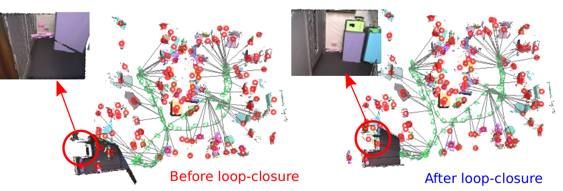
To evaluate the performance of our system while repeatedly viewing a scene of instances we captured a 3,685 frame sequence of an indoor office scene. We tailored this sequence to evaluate the consistency of our map in the presence of poorly constrained (planar floor) geometry and ICP drift, after which we loop over the same scene again. The pose-graph and loop closure is shown in Figure 5, it can be seen that despite the accumulated drift, the system re-localises and corrects the pose graph, this allows the previously reconstructed objects to be correctly associated in future frames. On the entirety of the trajectory our system reconstructed 105 landmark object instances, however, it must be noted that despite our filtering mechanisms, a build up of noisy partially reconstructed sub-objects still occurs.

To evaluate the reconstruction quality we use objects from the YCB dataset which provides ground truth models [1] and reconstruct discovered objects from sequence 0001 of the public YCB video dataset [41]. Figure 6 shows a qualitative comparison against the ground truth. The missing portion of the cracker box was caused by an occlusion by another object, and a missed foreground detection on one of the few frames where the cracker box was unoccluded.

We evaluate the trajectory error of our system against the baseline approach of simple coarse TSDF odometry, i.e. using the same coarse resetting background without instances layered on top, and without loop-closure pose graph optimisation. Table 1 shows the results. It can be seen that in all but one of the sequences evaluated our Fusion++ system improved upon the baseline approach (while providing an inventory of objects as Figure 1 visualises for the fr2_desk sequence). It is also worth noting that our system does not achieve state-of-the-art performance on these sequences such as [38, 22], and would require additional work, such as including joint depth and photometric tracking, to become competitive. We focused on a usable object map here and leave accuracy of motion tracking for future work.

Memory usage: We use the office sequence to evaluate the run-time performance and memory usage of our system. As memory usage scales cubically with the size of a TSDF, it is significantly more efficient to compose a map of many relatively small, highly detailed, volumes in dense areas of interest than to use one large one with a resolution equal to the smallest. After loading the CNN and image buffers, our remaining $\sim$7GB GPU memory budget (and 10 bytes per voxel) would allow a single $900^{3}$ volume or, as here, a $256^{3}$ background volume and up to 2.5K object volumes with dimension $64^{3}$, 2MB. Our object volumes dynamically vary up to $128^{3}$ and on our office sequence used 377MB for 105 objects ($\sim$4MB/object), as shown in Figure 7. Of course, more efficient alternatives such as an octree or voxel hashing can also be used to directly eliminate wasted free-space voxels, and are also directly applicable to our approach.

Runtime performance: Our system, although not real-time, scales well with the number of objects. Excluding re-localisation on the office sequence the average frame rate was 4-8Hz (shown in Figure 7), with an average additional computational cost of 1ms per object. A more detailed breakdown of the runtime performance of different components and their scaling factors is given in Table 2.

References

- [1] B. Calli, A. Singh, A. Walsman, P. Srinivasa S. and, Abbeel, and A. M. Dollar. The ycb object and model set: Towards common benchmarks for manipulation research. In International Conference on Advanced Robotics (ICAR), pages 510–517, 2015.
- [2] A. X. Chang, T. Funkhouser, L. Guibas, P. Hanrahan, Q. Huang, Z. Li, S. Savarese, M. Savva, S. Song, H. Su, J. Xiao, L. Yi, and F. Yu. ShapeNet: An information-rich 3d model repository. arXiv preprint arXiv:1512.03012, 2015.
- [3] S. Choi, Q. Zhou, and V. Koltun. Robust Reconstruction of Indoor Scenes. In Proceedings of the IEEE Conference on Computer Vision and Pattern Recognition (CVPR), 2015.
- [4] S. Choudhary, A. J. B. Trevor, H. I. Christensen, and F. Dellaert. SLAM with object discovery, modeling and mapping. In Proceedings of the IEEE/RSJ Conference on Intelligent Robots and Systems (IROS), 2014.
- [5] A. Collet, B. Xiong, C. Gurau, M. Hebert, and S. S. Srinivasa. Exploiting Domain Knowledge for Object Discovery. In Proceedings of the IEEE International Conference on Robotics and Automation (ICRA), 2013.
- [6] B. Curless and M. Levoy. A volumetric method for building complex models from range images. In Proceedings of SIGGRAPH, 1996.
- [7] A. Dai, , J. Sturm, and M. Nießner. Scancomplete: Large-scale scene completion and semantic segmentation for 3d scans. In Proceedings of the IEEE Conference on Computer Vision and Pattern Recognition (CVPR), 2018.
- [8] A. Dai, M. Nießner, M. Zollhöfer, S. Izadi, and C. Theobalt. BundleFusion: Real-time Globally Consistent 3D Reconstruction using On-the-fly Surface Re-integration. ACM Transactions on Graphics (TOG), 36(3):24:1–24:18, 2017.
- [9] T. Dharmasiri, V. Lui, and T. Drummond. MO-SLAM: Multi Object SLAM with Run-Time Object Discovery through Duplicates. In Proceedings of the IEEE/RSJ Conference on Intelligent Robots and Systems (IROS), 2016.
- [10] E. Eade. Lie groups for 2d and 3d transformations, 2017.
- [11] M. Fehr, F. Furrer, D. Ivan, J. Sturm, I. Gilitschenski, R. Siegwart, and C. Cadena. TSDF-based change detection for consistent long-term dense reconstruction and dynamic object discovery. In Proceedings of the IEEE International Conference on Robotics and Automation (ICRA), 2017.
- [12] R. Finman, T. Whelan, and M. Kaess. Toward lifelong object segmentation from change detection in dense RGB-D maps. In Proceedings of the European Conference on Mobile Robotics (ECMR), 2013.
- [13] K. He, G. Gkioxari, P. Dollár, and R. Girshick. Mask r-cnn. In Proceedings of the International Conference on Computer Vision (ICCV), 2017.
- [14] K. He, X. Zhang, S. Ren, and J. Sun. Deep residual learning for image recognition. In Proceedings of the IEEE Conference on Computer Vision and Pattern Recognition (CVPR), 2016.
- [15] A. Hermans, G. Floros, and B. Leibe. Dense 3d semantic mapping of indoor scenes from rgb-d images. In Proceedings of the IEEE International Conference on Robotics and Automation (ICRA), 2014.
- [16] L. Kneip and P. Furgale. Opengv: A unified and generalized approach to real-time calibrated geometric vision. In Proceedings of the IEEE International Conference on Robotics and Automation (ICRA), 2014.
- [17] R. Kümmerle, G. Grisetti, H. Strasdat, K. Konolige, and W. Burgard. : A General Framework for Graph Optimization. In Proceedings of the IEEE International Conference on Robotics and Automation (ICRA), 2011.
- [18] S. Leutenegger, M. Chli, and R. Siegwart. BRISK: Binary robust invariance scalable keypoints. In Proceedings of the International Conference on Computer Vision (ICCV), 2011.
- [19] L. Ma and G. Sibley. Unsupervised Dense Object Discovery, Detection, Tracking and Reconstruction. In Proceedings of the European Conference on Computer Vision (ECCV), 2014.
- [20] J. McCormac, A. Handa, A. J. Davison, and S. Leutenegger. SemanticFusion: Dense 3D semantic mapping with convolutional neural networks. In Proceedings of the IEEE International Conference on Robotics and Automation (ICRA), 2017.
- [21] R. Mur-Artal and J. D. Tardós. ORB-SLAM: Tracking and Mapping Recognizable Features. In Workshop on Multi View Geometry in Robotics (MVIGRO) - RSS 2014, 2014.
- [22] R. Mur-Artal and J. D. Tardós. ORB-SLAM2: An Open-Source SLAM System for Monocular, Stereo, and RGB-D Cameras. IEEE Transactions on Robotics (T-RO), 33(5):1255–1262, 2017.
- [23] R. A. Newcombe, S. Izadi, O. Hilliges, D. Molyneaux, D. Kim, A. J. Davison, P. Kohli, J. Shotton, S. Hodges, and A. Fitzgibbon. KinectFusion: Real-Time Dense Surface Mapping and Tracking. In Proceedings of the International Symposium on Mixed and Augmented Reality (ISMAR), 2011.
- [24] R. A. Newcombe, S. Lovegrove, and A. J. Davison. DTAM: Dense Tracking and Mapping in Real-Time. In Proceedings of the International Conference on Computer Vision (ICCV), 2011.
- [25] Q. Pham, B. Hua, D. T. Nguyen, and S. Yeung. Real-time progressive 3d semantic segmentation for indoor scenes. arXiv preprint arXiv:1804.00257, 2018.
- [26] S. Pillai and J. J. Leonard. Monocular SLAM Supported Object Recognition. In Proceedings of Robotics: Science and Systems (RSS), 2015.
- [27] S. Ren, K. He, R. Girshick, and J. Sun. Faster r-cnn: Towards real-time object detection with region proposal networks. In Neural Information Processing Systems (NIPS), pages 91–99, 2015.
- [28] E. Rublee, V. Rabaud, K. Konolige, and G. Bradski. ORB: an efficient alternative to SIFT or SURF. In Proceedings of the International Conference on Computer Vision (ICCV), pages 2564–2571. IEEE, 2011.
- [29] M. Rünz and L. Agapito. Maskfusion: Real-time recognition, tracking and reconstruction of multiple moving objects. arXiv preprint arXiv:1804.09194, 2018.
- [30] R. F. Salas-Moreno, R. A. Newcombe, H. Strasdat, P. H. J. Kelly, and A. J. Davison. SLAM++: Simultaneous Localisation and Mapping at the Level of Objects. In Proceedings of the IEEE Conference on Computer Vision and Pattern Recognition (CVPR), 2013.
- [31] J. Stückler and S. Behnke. Model learning and real-time tracking using multi-resolution surfel maps. In Proceedings of the National Conference on Artificial Intelligence (AAAI), 2012.
- [32] J. Stückler and S. Behnke. Hierarchical object discovery and dense modelling from motion cues in RGB-D video. In Proceedings of the International Joint Conference on Artificial Intelligence (IJCAI), 2013.
- [33] J. Sturm, N. Engelhard, F. Endres, W. Burgard, and D. Cremers. A Benchmark for the Evaluation of RGB-D SLAM Systems. In Proceedings of the IEEE/RSJ Conference on Intelligent Robots and Systems (IROS), 2012.
- [34] N. Sünderhauf, T. T. Pham, Y. Latif, M. Milford, and I. Reid. Meaningful maps with object-oriented semantic mapping. In Proceedings of the IEEE/RSJ Conference on Intelligent Robots and Systems (IROS), 2017.
- [35] K. Tateno, F. Tombari, and N. Navab. When 2.5D is not enough: Simultaneous reconstruction, segmentation and recognition on dense slam. In Proceedings of the IEEE International Conference on Robotics and Automation (ICRA), 2016.
- [36] A. Trevor, S. Gedikli, R. Rusu, and H. Christensen. Efficient Organized Point Cloud Segmentation with Connected Components. In 3rd Workshop on Semantic Perception Mapping and Exploration (SPME), 2013.
- [37] T. Whelan, M. Kaess, H. Johannsson, M. F. Fallon, J. J. Leonard, and J. B. McDonald. Real-time large scale dense RGB-D SLAM with volumetric fusion. International Journal of Robotics Research (IJRR), 34(4-5):598–626, 2015.
- [38] T. Whelan, S. Leutenegger, R. F. Salas-Moreno, B. Glocker, and A. J. Davison. ElasticFusion: Dense SLAM without a pose graph. In Proceedings of Robotics: Science and Systems (RSS), 2015.
- [39] T. Whelan, J. B. McDonald, M. Kaess, M. Fallon, H. Johannsson, and J. J. Leonard. Kintinuous: Spatially Extended KinectFusion. In Workshop on RGB-D: Advanced Reasoning with Depth Cameras, in conjunction with Robotics: Science and Systems, 2012.
- [40] Y. Wu et al. Tensorpack. https://github.com/tensorpack/, 2016.
- [41] Y. Xiang, T. Schmidt, V. Narayanan, and D. Fox. Posecnn: A convolutional neural network for 6d object pose estimation in cluttered scenes. arXiv preprint arXiv:1711.00199, 2017.
- [42] Q. Zhou and V. Koltun. Dense scene reconstruction with points of interest. In Proceedings of SIGGRAPH, 2013.
- [43] Q. Zhou, S. Miller, and V. Koltun. Elastic Fragments for Dense Scene Reconstruction. In Proceedings of the International Conference on Computer Vision (ICCV), 2013.