跳到论文正文
W Papers独立论文阅读器 arXiv:1808.07974 论文正文 计算阅读时间 · 0%
引用这篇论文根据当前论文元数据生成,正式投稿前建议核对。


License: arXiv.org perpetual non-exclusive license
arXiv:1808.07974v1 [math.CA] 24 Aug 2018

Stability of scalar nonlinear fractional differential equations with linearly dominated delay

H.T. Tuan Note: httuan@math.ac.vn, Institute of Mathematics, Vietnam Academy of Science and Technology, 18 Hoang Quoc Viet, 10307 Ha Noi, Viet Nam    S. Siegmund Note: stefan.siegmund@tu-dresden.de, Center for Dynamics, Faculty of Mathematics, TU Dresden, 01069 Dresden, Germany
Abstract

In this paper, we study the asymptotic behavior of solutions to a scalar fractional delay differential equations around the equilibrium points. More precise, we provide conditions on the coefficients under which a linear fractional delay equation is asymptotically stable and show that the asymptotic stability of the trivial solution is preserved under a small nonlinear Lipschitz perturbation of the fractional delay differential equation.

1 Introduction

Let A,B∈ℝd×dA,B\in\mathbb{R}^{d\times d} and f:ℝd×ℝd→ℝdf:\mathbb{R}^{d}\times\mathbb{R}^{d}\rightarrow\mathbb{R}^{d} be locally Lipschitz continuous. The existence of solutions of the Caputo fractional differential equation

D0+αC​x​(t)=A​x​(t)+B​x​(t−τ)+f⁡(x⁡(t),x⁡(t−τ)){}^{\rm{\scriptscriptstyle C\!\!}}D^{\alpha}_{0+}x(t)=Ax(t)+Bx(t-\tau)+f(x(t),x(t-\tau)) (1)

of order α∈(0,1)\alpha\in(0,1) with delay τ>0\tau>0 and continuous initial condition x⁡(t)=ϕ⁡(t)x(t)=\phi(t), t∈[−τ,0]t\in[-\tau,0], has been studied in many papers. Abbas [1] used Krasnoselskii’s fixed point theorem to show the existence of at least one local solution. Jalilian and Jalilian [15] proved the existence of a global solution on a finite interval by using a fixed point theorem of Leray–Schauder type. Using properties of Mittag-Leffler functions, a weighted norm, and the Banach fixed point theorem, Cong and Tuan [5] established the existence and uniqueness of global solutions under a mild Lipschitz condition.

Whenever solutions exist, it is of particular importance to understand their asymptotic behavior. To the best of our knowledge, up to now, there have been only very few contributions to the qualitative theory of (1). For f=0f=0 and B=0B=0, Matignon [12] has given a well-known stability criterion based on the spectrum of the matrix AA. Cermak, Hornicek and Kisela [3] studied the case f=0f=0, A=0A=0, and obtained a necessary and sufficient condition for the stability of this system. The stability of the system when A=0A=0 was discussed by Tuan and Hieu in [18]. Regarding the asymptotic behavior of solutions to (1) for f=0f=0, d=1d=1, Stamova [17], Cermak, Dosla, Kisela [4] and He et al. [10] provided results to characterize the stability of solutions. In the case f=0f=0 and d≥1d\geq 1, Shen and Lam [16] considered the stability and performance analysis of the system with the assumptions AA is Metzler and BB is nonnegative. Recently, using the properties of Caputo fractional derivatives, the Laplace transform and the Mittag-Leffler function, Thanh, Hieu and Phat [19] proposed sufficient conditions for exponential boundedness, asymptotic stability and finite-time stability of (1) for f=0f=0 and A,BA,B arbitrary. However, in contrast to fractional differential equations without delays, the stability theory of delay fractional differential equations (1) is far from being fully understood.

In this paper we answer the open question about the relationship between the stability of the trivial solution of (1) and that of its linearization in the scalar case d=1d=1. More precise, we consider the scalar delay fractional differential equation

Dα0+C​x​(t)=a​x​(t)+b​x​(t−τ)+f⁡(x⁡(t),x⁡(t−τ)){}^{\rm{\scriptscriptstyle C\!\!}}D_{0+}^{\alpha}x(t)=ax(t)+bx(t-\tau)+f(x(t),x(t-\tau)) (2)

where f:ℝ2→ℝf\colon\mathbb{R}^{2}\rightarrow\mathbb{R} is locally Lipschitz continuous and satisfies the following conditions:

  • (H1)

    Trivial solution: f⁡(0,0)=0f(0,0)=0,

  • (H2)

    Nonlinearity: limϱ→0ℓf​(ϱ)=0\lim_{\varrho\to 0}\ell_{f}(\varrho)=0 with

    ℓf​(ϱ)≔supx,y,x^,y^∈Bℝ​(0,ϱ)(x,y)≠(x^,y^)|f⁡(x,y)−f⁡(x^,y^)|max⁡{|x−x^|,|y−y^|}.\ell_{f}(\varrho)\coloneqq\sup_{\begin{subarray}{c}x,y,\hat{x},\hat{y}\in B_{\mathbb{R}}(0,\varrho)\\ (x,y)\neq(\hat{x},\hat{y})\end{subarray}}\frac{|f(x,y)-f(\hat{x},\hat{y})|}{\max\{|x-\hat{x}|,|y-\hat{y}|\}}.

As shown in [1, Theorem 2.6], for every continuous initial function ϕ:[−τ,0]→ℝ\phi\colon[-\tau,0]\rightarrow\mathbb{R}, there exists a unique continuous solution φ(⋅,ϕ):[−τ,tmax(ϕ))→ℝ\varphi(\cdot,\phi)\colon[-\tau,t_{\max}(\phi))\to\mathbb{R} to (2) on the maximal interval of existence [−τ,tmax(ϕ))[-\tau,t_{\max}(\phi)) which satisfies the initial condition

x⁡(t)=ϕ⁡(t),t∈[−τ,0].x(t)=\phi(t),\qquad t\in[-\tau,0]. (3)

By (H1), equation (2) admits the trivial solution

φ(⋅,0):[−τ,∞)→ℝ,t↦0.\varphi(\cdot,0)\colon[-\tau,\infty)\to\mathbb{R},\quad t\mapsto 0.

For an interval I⊆ℝI\subseteq\mathbb{R}, let C⁡(I,ℝ)C(I;\mathbb{R}) denote the set of continuous functions x:I→ℝx\colon I\to\mathbb{R} with ‖x‖∞≔supt∈I|x⁡(t)|\|x\|_{\infty}\coloneqq\sup_{t\in I}|x(t)|. As in [18, Definition 1], the trivial solution of (2) is called

stable ⇔∀ε>0​∃δ>0​∀ϕ∈C⁡([−τ,0],ℝ)​ with ​‖ϕ‖∞≤δ:\displaystyle\ratio\Leftrightarrow\forall\varepsilon>0\,\exists\delta>0\,\forall\phi\in C([-\tau,0];\mathbb{R})\text{ with }\|\phi\|_{\infty}\leq\delta\colon
tmax​(ϕ)=∞​ and ​|φ⁡(t,ϕ)|≤ε​ for ​t∈[0,∞),\displaystyle\qquad t_{\max}(\phi)=\infty\text{ and }|\varphi(t,\phi)|\leq\varepsilon\text{ for }t\in[0,\infty),
attractive ⇔∃δ>0​∀ϕ∈C⁡([−τ,0],ℝ)​ with ​‖ϕ‖∞≤δ:\displaystyle\ratio\Leftrightarrow\exists\delta>0\,\forall\phi\in C([-\tau,0];\mathbb{R})\text{ with }\|\phi\|_{\infty}\leq\delta\colon
tmax​(ϕ)=∞​ and ​limt→∞φ⁡(t,ϕ)=0,\displaystyle\qquad t_{\max}(\phi)=\infty\text{ and }\lim_{t\to\infty}\varphi(t,\phi)=0,

and

asymptotically stable ⇔the trivial solution is stable and attractive.\displaystyle\ratio\Leftrightarrow\text{the trivial solution is stable and attractive.}

In Section 5 we provide conditions on aa, bb and ff which imply asymptotic stability of the trivial solution of (2). To prepare the proof of this main result, we show a variation of constants formula for (2) in Section 2, properties of the characteristic function in Section 3 and estimates for the Mittag-Leffler function in Section 4.

A reader who is familiar with fractional difference equations may skip the remainder of this section, in which we recall notation. Let T>0T>0 and x:[0,T]→ℝx\colon[0,T]\to\mathbb{R} be a measurable function in L1​([0,T])L^{1}([0,T]), i.e. ∫0T|x⁡(s)|​𝑑s<∞\int_{0}^{T}|x(s)|\;ds<\infty. Then, the Riemann–Liouville integral of order α>0\alpha>0 is defined by

I0+α​x​(t):=1Γ⁡(α)​∫0t(t−s)α−1​x​(s)​𝑑s for ​t∈(0,T],I_{0+}^{\alpha}x(t):=\frac{1}{\Gamma(\alpha)}\int_{0}^{t}(t-s)^{\alpha-1}x(s)\;ds\quad\hbox{ for }t\in(0,T],

where the Gamma function Γ:(0,∞)→ℝ\Gamma:(0,\infty)\rightarrow\mathbb{R} is defined as

Γ⁡(α):=∫0∞sα−1​exp⁡(−s)​𝑑s,\Gamma(\alpha):=\int_{0}^{\infty}s^{\alpha-1}\exp(-s)\;ds,

see e.g., Diethelm [8]. The corresponding Riemann–Liouville fractional derivative of order α\alpha is given by

Dα0+R​-​L​x​(t):=(D​I0+1−α​x)​(t)for almost all ​t∈(0,T],{}^{\rm{\scriptscriptstyle R\text{-}L\!\!}}D_{0+}^{\alpha}x(t):=(DI_{0+}^{1-\alpha}x)(t)\quad\text{for almost all }t\in(0,T],

where D=dd​tD=\frac{d}{dt} is the usual derivative. The Caputo fractional derivative Dα0+C​x{}^{\rm{\scriptscriptstyle C\!\!}}D_{0+}^{\alpha}x of a continuous function x:[0,T]→ℝx\colon[0,T]\to\mathbb{R} is defined by

Dα0+C​x​(t)≔Dα0+R​-​L​(x⁡(t)−x⁡(0))for almost all ​t∈(0,T].{}^{\rm{\scriptscriptstyle C\!\!}}D_{0+}^{\alpha}x(t)\coloneqq{}^{\rm{\scriptscriptstyle R\text{-}L\!\!}}D_{0+}^{\alpha}(x(t)-x(0))\quad\text{for almost all }t\in(0,T].

In a normed space (X,∥⋅∥)(X,\|\cdot\|) we denote the closed ball with radius ϱ>0\varrho>0 centered at the origin by BX​(0,ϱ)B_{X}(0,\varrho).

2 Variation of constants formula

In the case f=0f=0, the linear initial value problem (2), (3), with continuous initial function ϕ:[−τ,0]→ℝ\phi\colon[-\tau,0]\to\mathbb{R}, has the solution

φ⁡(t,ϕ)=ϕ⁡(0)​Eα,1a,b,τ​(t)+b​∫−τt−τEα,αa,b,τ​(t−τ−s)​ϕ~​(s)​𝑑s,\varphi(t,\phi)=\phi(0)E^{a,b,\tau}_{\alpha,1}(t)+b\int_{-\tau}^{t-\tau}E^{a,b,\tau}_{\alpha,\alpha}(t-\tau-s)\tilde{\phi}(s)ds,

where

Eα,βa,b,τ​(t):=ℒ−1​(sα−βsα−a−b​exp⁡(−s​τ))​(t),E^{a,b,\tau}_{\alpha,\beta}(t):=\mathcal{L}^{-1}\Big(\frac{s^{\alpha-\beta}}{s^{\alpha}-a-b\exp{(-s\tau)}}\Big)(t),

β=1\beta=1 or β=α\beta=\alpha, ℒ−1\mathcal{L}^{-1} is the inverse Laplace transform, ϕ~\tilde{\phi} is the function defined by

ϕ~​(t)={ϕ⁡(t),if​t∈[−τ,0],0,if​t>0.\tilde{\phi}(t)=\begin{cases}\phi(t),&\text{if}\;t\in[-\tau,0],\\ 0,&\text{if}\;t>0.\end{cases}

If ff is globally Lipschitz continuous, using the Laplace transform and the arguments as in [3, Theorem 3], [7, Lemma 3.1], and [18, Lemma 1], we obtain the following variation of constants formula for (2).

Lemma 2.1 (Variation of constants formula for delay fractional differential equations).

Assume that f:ℝ×ℝ→ℝf:\mathbb{R}\times\mathbb{R}\to\mathbb{R} is Lipschitz continuous and ϕ:[−τ,0]→ℝ\phi:[-\tau,0]\to\mathbb{R} is continuous. Then, equation (2) with the initial condition (3) has a unique solution φ⁡(⋅,ϕ)\varphi(\cdot,\phi) on [−τ,∞)[-\tau,\infty). Moreover, this solution satisfies

φ⁡(t,ϕ)\displaystyle\varphi(t,\phi) =ϕ⁡(0)​Eα,1a,b,τ​(t)+b​∫−τt−τEα,αa,b,τ​(t−τ−s)​ϕ~​(τ)​𝑑τ\displaystyle=\phi(0)E^{a,b,\tau}_{\alpha,1}(t)+b\int_{-\tau}^{t-\tau}E^{a,b,\tau}_{\alpha,\alpha}(t-\tau-s)\tilde{\phi}(\tau)d\tau
+∫0tEα,αa,b,τ(t−s)f(φ(s),φ(s−τ))dsfor t>0.\displaystyle\hskip 14.22636pt+\int_{0}^{t}E^{a,b,\tau}_{\alpha,\alpha}(t-s)f(\varphi(s),\varphi(s-\tau))ds\quad\text{for }t>0. (4)
Proof.

From [5, Corollary 3.2], we see that for any continuous initial data ϕ\phi, equation (2) with the initial condition x⁡(t)=ϕ⁡(t)x(t)=\phi(t) on [−τ,0][-\tau,0] has a unique solution on [−τ,∞)[-\tau,\infty). Moreover, this solution is exponentially bounded, see [5, Theorem 4.1]. Taking the Laplace transform on both sides of (2) and using the facts that

ℒ⁡(D0+αC​x​(t))​(s)\displaystyle\mathcal{L}({}^{\rm{\scriptscriptstyle C\!\!}}D^{\alpha}_{0+}x(t))(s) =sα​ℒ​(x⁡(t))​(s)−sα−1​x​(0)=sα​X​(s)−sα−1​ϕ​(0),\displaystyle=s^{\alpha}\mathcal{L}(x(t))(s)-s^{\alpha-1}x(0)=s^{\alpha}X(s)-s^{\alpha-1}\phi(0),
ℒ​(x​(t−τ)​(s)CLOSE\displaystyle\mathcal{L}(x(t-\tau)(s) =exp⁡(−τ​s)​ℒ​(x⁡(t))​(s)+exp⁡(−τ​s)​∫−τ0exp⁡(−s​u)​x​(u)​𝑑u\displaystyle=\exp{(-\tau s)}\mathcal{L}(x(t))(s)+\exp{(-\tau s)}\int_{-\tau}^{0}\exp{(-su)}x(u)\;du
=exp⁡(−τ​s)​X​(s)+exp⁡(−τ​s)​∫−τ0exp⁡(−s​u)​ϕ​(u)​𝑑u,\displaystyle=\exp{(-\tau s)}X(s)+\exp{(-\tau s)}\int_{-\tau}^{0}\exp{(-su)}\phi(u)\;du,

for s∈{z∈ℂ:ℜ⁡z>c}s\in\{z\in\mathbb{C}:\Re z>c\}, cc large enough, we get

X⁡(s)\displaystyle X(s) =sα−1​ϕ​(0)sα−a−b​exp⁡(−τ​s)+b​exp⁡(−τ​s)​∫−τ0exp⁡(−s​u)​ϕ​(u)​𝑑usα−a−b​exp⁡(−τ​s)\displaystyle=\frac{s^{\alpha-1}\phi(0)}{s^{\alpha}-a-b\exp{(-\tau s)}}+\frac{b\exp{(-\tau s)}\int_{-\tau}^{0}\exp{(-su)}\phi(u)\;du}{s^{\alpha}-a-b\exp{(-\tau s)}}
+F⁡(s)sα−a−b​exp⁡(−τ​s),\displaystyle\quad{}+\frac{F(s)}{s^{\alpha}-a-b\exp{(-\tau s)}}, (5)

where X​(s)≔ℒ​(x​(t))​(s)X(s)\coloneqq\mathcal{L}(x(t))(s) and F⁡(s)=ℒ⁡(f⁡(x⁡(t),x⁡(t−τ)))​(s)F(s)=\mathcal{L}(f(x(t),x(t-\tau)))(s). Applying the inverse Laplace transform on both sides of (5), we obtain

x⁡(t)\displaystyle x(t) =Eα,1a,b,τ​(t)​ϕ​(0)+b​∫−τt−τEα,αa,b​τ​(t−τ−s)​ϕ~​(s)​𝑑s\displaystyle=E^{a,b,\tau}_{\alpha,1}(t)\phi(0)+b\int_{-\tau}^{t-\tau}E^{a,b\,\tau}_{\alpha,\alpha}(t-\tau-s)\tilde{\phi}(s)\;ds
+∫0tEα,αa,b,τ(t−s)f(x(s),x(s−τ))dsfor t>0.\displaystyle\quad{}+\int_{0}^{t}E^{a,b,\tau}_{\alpha,\alpha}(t-s)f(x(s),x(s-\tau))\;ds\quad\text{for }t>0. (6)

Here, to obtain (6), we used

ℒ−1​(F⁡(s)sα−a−b​exp⁡(−τ​s))​(t)\displaystyle\mathcal{L}^{-1}\left(\frac{F(s)}{s^{\alpha}-a-b\exp{(-\tau s)}}\right)(t) =ℒ−1​(F⁡(s)​ℒ​(Eα,αa,b,τ​(t))​(s))​(t)\displaystyle=\mathcal{L}^{-1}\left(F(s)\mathcal{L}(E^{a,b,\tau}_{\alpha,\alpha}(t))(s)\right)(t)
=ℒ−1(ℒ(f(x(⋅),x(⋅−τ))∗Eα,αa,b,τ(⋅)(t))(s))(t)\displaystyle=\mathcal{L}^{-1}\left(\mathcal{L}(f(x(\cdot),x(\cdot-\tau))\ast E^{a,b,\tau}_{\alpha,\alpha}(\cdot)(t))(s)\right)(t)
=∫0tEα,αa,b,τ​(t−s)​f​(x⁡(s),x⁡(s−τ))​𝑑s,\displaystyle=\int_{0}^{t}E^{a,b,\tau}_{\alpha,\alpha}(t-s)f(x(s),x(s-\tau))\;ds,

and

ℒ−1​(exp⁡(−τ​s)​∫−τ0exp⁡(−s​u)​ϕ​(u)​𝑑usα−a−b​exp⁡(−τ​s))​(t)\displaystyle\mathcal{L}^{-1}\left(\frac{\exp{(-\tau s)}\int_{-\tau}^{0}\exp{(-su)}\phi(u)\;du}{s^{\alpha}-a-b\exp{(-\tau s)}}\right)(t)
=ℒ−1​(ℒ⁡(Eα,αa,b​τ​(t))​(s)​ℒ​(ϕ~​(t−τ))​(s))​(t)\displaystyle\hskip 56.9055pt=\mathcal{L}^{-1}\left(\mathcal{L}(E^{a,b\,\tau}_{\alpha,\alpha}(t))(s)\mathcal{L}(\tilde{\phi}(t-\tau))(s)\right)(t)
=ℒ−1(ℒ(Eα,αa,b​τ(⋅)∗ϕ~(⋅−τ)(t))(s))(t)\displaystyle\hskip 56.9055pt=\mathcal{L}^{-1}\left(\mathcal{L}(E^{a,b\,\tau}_{\alpha,\alpha}(\cdot)\ast\tilde{\phi}(\cdot-\tau)(t))(s)\right)(t)
=∫−τt−τEα,αa,b​τ​(t−τ−s)​ϕ~​(s)​𝑑s,\displaystyle\hskip 56.9055pt=\int_{-\tau}^{t-\tau}E^{a,b\,\tau}_{\alpha,\alpha}(t-\tau-s)\tilde{\phi}(s)\;ds,

where ∗\ast denotes the convolution operator. ∎

3 Properties of the characteristic function

To derive the asymptotic behavior of the solutions to (2) from (4), we need to study the function Eα,βa,b,τ​(t)E^{a,b,\tau}_{\alpha,\beta}(t). First, we recall some facts concerning the zeros of the characteristic function Q⁡(s):=sα−a−b​exp⁡(−s​τ)Q(s):=s^{\alpha}-a-b\exp{(-s\tau)}.

Lemma 3.1.

Let α∈(0,1)\alpha\in(0,1), a,b∈ℝa,b\in\mathbb{R}, τ>0\tau>0. Then the following statements hold.

  • (i)

    If a+b≥0a+b\geq 0, then the equation Q⁡(s)=0Q(s)=0 has at least one nonnegative real root.

  • (ii)

    If ss is a zero of QQ, then its complex conjugate s¯\bar{s} also satisfies Q⁡(s¯)=0Q(\bar{s})=0.

  • (iii)

    Let 0<ω<π0<\omega<\pi. Then the equation Q⁡(s)=0Q(s)=0 has at most finitely many roots ss such that |arg⁡(s)|≤ω|\arg(s)|\leq\omega.

  • (iv)

    The equation Q⁡(s)=0Q(s)=0 has no more than a finite number of roots in any vertical strip of the complex plane given by

    {z∈ℂ:ρ1≤ℜ⁡(z)≤ρ2}.\{z\in\mathbb{C}\colon\rho_{1}\leq\Re{(z)}\leq\rho_{2}\}.
  • (v)

    There does not exist an s∈ℂ∖{0}s\in\mathbb{C}\setminus\{0\} satisfying Q⁡(s)=Q′​(s)=Q′′​(s)=Q′′′​(s)=0Q(s)=Q^{\prime}(s)=Q^{\prime\prime}(s)=Q^{\prime\prime\prime}(s)=0.

Proof.

For the proof of (i)–(iii), see [4, Proposition 2].

(iv) Assume that s=x+i​y∈{z∈ℂ:ρ1≤ℜ⁡(z)≤ρ2}s=x+iy\in\{z\in\mathbb{C}\colon\rho_{1}\leq\Re{(z)}\leq\rho_{2}\}. Choosing T0>0T_{0}>0 such that T0α>|a|+|b|​exp⁡(−ρ1​τ)T^{\alpha}_{0}>|a|+|b|\exp{(-\rho_{1}\tau)}. Then, for any s=x+i​y∈{z∈ℂ:ρ1≤ℜ⁡(z)≤ρ2}∩{z∈ℂ:|ℑ⁡(z)|≥T0}s=x+iy\in\{z\in\mathbb{C}\colon\rho_{1}\leq\Re{(z)}\leq\rho_{2}\}\cap\{z\in\mathbb{C}\colon|\Im{(z)}|\geq T_{0}\}, we have

|sα|>|a|+|b|​|exp⁡(−s​τ)|,|s^{\alpha}|>|a|+|b|\;|\exp{(-s\tau)}|,

which implies that the equation Q⁡(s)=0Q(s)=0 has no solution in the set {z∈ℂ:ρ1≤ℜ⁡(z)≤ρ2}∩{z∈ℂ:|ℑ⁡(z)|≥T0}\{z\in\mathbb{C}\colon\rho_{1}\leq\Re{(z)}\leq\rho_{2}\}\cap\{z\in\mathbb{C}\colon|\Im(z)|\geq T_{0}\}. On the other hand, the function Q⁡(s)Q(s) has only finitely many roots in the compact set {z=x+iy∈ℂ:ρ1≤x≤ρ2,−T0≤y≤T0}\{z=x+iy\in\mathbb{C}\colon\rho_{1}\leq x\leq\rho_{2},\;-T_{0}\leq y\leq T_{0}\} (the function QQ is analytic in this domain). Hence, there exist at most finitely many roots of Q⁡(s)Q(s) in {z∈ℂ:ρ1≤ℜ⁡(z)≤ρ2}.\{z\in\mathbb{C}\colon\rho_{1}\leq\Re{(z)}\leq\rho_{2}\}.

(v) Now we assume that there exists s∈ℂ∖{0}s\in\mathbb{C}\setminus\{0\} such that Q⁡(s)=Q′​(s)=Q′′​(s)=Q′′′​(s)=0Q(s)=Q^{\prime}(s)=Q^{\prime\prime}(s)=Q^{\prime\prime\prime}(s)=0. Using Q′​(s)=Q′′​(s)=0Q^{\prime}(s)=Q^{\prime\prime}(s)=0, a direct computation shows

b​exp⁡(−τ​s)=−α​sα−1τ=α⁡(α−1)​sα−2τ2,b\exp{(-\tau s)}=-\frac{\alpha s^{\alpha-1}}{\tau}=\frac{\alpha(\alpha-1)s^{\alpha-2}}{\tau^{2}},

which implies

s=1−ατ.s=\frac{1-\alpha}{\tau}. (7)

Similarly, from the equality Q′′​(s)=Q′′′​(s)=0Q^{\prime\prime}(s)=Q^{\prime\prime\prime}(s)=0, we have

b​exp⁡(−τ​s)=α⁡(α−1)​sα−2τ2=−α⁡(α−1)​(α−2)​sα−3τ3,b\exp{(-\tau s)}=\frac{\alpha(\alpha-1)s^{\alpha-2}}{\tau^{2}}=-\frac{\alpha(\alpha-1)(\alpha-2)s^{\alpha-3}}{\tau^{3}},

which implies

s=2−ατ,s=\frac{2-\alpha}{\tau},

a contradiction to (7). The proof of (iv) completes. ∎

The following lemma provides a condition which ensures that all solutions s∈ℂs\in\mathbb{C} of Q⁡(s)=0Q(s)=0 satisfy ℜ⁡(s)<0\Re(s)<0. It is stated without proof in [4, Proposition 4], we give a simple and geometric proof for completeness.

Lemma 3.2.

Let α∈(0,1)\alpha\in(0,1), a,b∈ℝa,b\in\mathbb{R} and τ>0\tau>0. If a≤b<−aa\leq b<-a, then the equation Q⁡(s)=0Q(s)=0 has no root with non-negative real part.

Proof.

Define C+≔{z∈ℂ:ℜ⁡(z)≥0}C_{+}\coloneqq\{z\in\mathbb{C}:\Re(z)\geq 0\} and the functions w1:C+→ℂw_{1}\colon C_{+}\to\mathbb{C}, w1​(s)=a+b​exp⁡(−τ​s)w_{1}(s)=a+b\exp{(-\tau s)} and w2:C+→ℂw_{2}\colon C_{+}\to\mathbb{C}, w2​(s)=sαw_{2}(s)=s^{\alpha}. It is obvious that D2≔w2​(C+)={s∈ℂ:|arg⁡(s)|≤α​π2}D_{2}\coloneqq w_{2}(C_{+})=\{s\in\mathbb{C}\colon|\arg(s)|\leq\frac{\alpha\pi}{2}\}. On the other hand, for any s∈C+s\in C_{+},

|w1​(s)−a|≤|b|.|w_{1}(s)-a|\leq|b|.

Hence, D1≔w1​(C+)={s∈ℂ:|s−a|≤|b|}D_{1}\coloneqq w_{1}(C_{+})=\{s\in\mathbb{C}\colon|s-a|\leq|b|\}. This shows that if a<0a<0 and |b|<|a||b|<|a| then D1∩D2=∅D_{1}\cap D_{2}=\emptyset (see Figure 1), that is, there does not exist s∈C+s\in C_{+} such that w1​(s)=w2​(s)w_{1}(s)=w_{2}(s). Now we consider a<0a<0 and a=ba=b. In this case D1∩D2={0}D_{1}\cap D_{2}=\{0\}. Assume that there is a s∈C+s\in C_{+} such that w1​(s)=w2​(s)w_{1}(s)=w_{2}(s). Then w2​(s)=0w_{2}(s)=0 which implies s=0s=0. However, w1​(0)≠0w_{1}(0)\neq 0, a contradiction. Combining the arguments as above, we conclude that if a≤b<|a|a\leq b<|a| then the equation Q⁡(s)=0Q(s)=0 has no solution with non-negative real part. ∎

‘

Figure 1: The domains D1D_{1} and D2D_{2} in the case a<0,|b|<|a|a<0,\;|b|<|a|.

4 Asymptotics of Mittag-Leffler functions

In the following lemma, we provide some estimates involving Mittag-Leffler functions Eα,βa,b,τ​(t)E^{a,b,\tau}_{\alpha,\beta}(t) under assumptions which ensure that all roots of the equation Q⁡(s)=0Q(s)=0 have negative real parts.

Lemma 4.1.

Let α∈(0,1)\alpha\in(0,1), τ>0\tau>0 and a,b∈ℝa,b\in\mathbb{R} satisfying a≤b<−aa\leq b<-a. Then, there exists a constant C>0C>0 such that the following estimates hold:

  • (i)

    |Eα,1a,b,τ​(t)|≤Ctα|E^{a,b,\tau}_{\alpha,1}(t)|\leq\frac{C}{t^{\alpha}} for all t≥1t\geq 1.

  • (ii)

    |Eα,αa,b,τ​(t)|≤Ctα+1|E^{a,b,\tau}_{\alpha,\alpha}(t)|\leq\frac{C}{t^{\alpha+1}} for all t≥1t\geq 1.

  • (iii)

    ∫0∞|Eα,αa,b,τ​(s)|​𝑑s≤C\int_{0}^{\infty}|E^{a,b,\tau}_{\alpha,\alpha}(s)|ds\leq C.

Proof.

In the case b=0b=0, the function Eα,βa,0,τ​(t)E^{a,0,\tau}_{\alpha,\beta}(t) equals tβ−1​Eα,β​(a​tα)t^{\beta-1}E_{\alpha,\beta}(at^{\alpha}) and this lemma is proved in [6, Theorems 2 & 3]. Hence, we only discuss the remaining case a≤b<−a,b≠0a\leq b<-a,\;b\neq 0.

We define for μ>0\mu>0 and θ∈(0,π)\theta\in(0,\pi) an oriented contour γ⁡(μ,θ)\gamma(\mu,\theta) formed by three segments:

  • •

    {s∈ℂ:arg(s)=−θ,|s|≥μ}\{s\in\mathbb{C}\colon\arg{(s)}=-\theta,|s|\geq\mu\},

  • •

    {s∈ℂ:−θ≤arg(s)≤θ,|s|=μ}\{s\in\mathbb{C}\colon-\theta\leq\arg{(s)}\leq\theta,|s|=\mu\},

  • •

    {s∈ℂ:arg(s)=θ,|s|≥μ}\{s\in\mathbb{C}\colon\arg{(s)}=\theta,|s|\geq\mu\},

Figure 2: The contour γ⁡(μ,θ)\gamma(\mu,\theta).

see Figure 2. By Lemma 3.1(iii), there exists a δ>0\delta>0 such that the function sα−a−b​exp⁡(−τ​s)s^{\alpha}-a-b\exp{(-\tau s)} has no zeros sis_{i} with |arg⁡(si)|=π2+δ|\arg{(s_{i})}|=\frac{\pi}{2}+\delta, and there are only finitely many zeros sis_{i} which satisfy |arg⁡(si)|≤π2+δ|\arg{(s_{i})}|\leq\frac{\pi}{2}+\delta. Hence, there exist R>0R>0 such that all zeros sis_{i} lie to the left of γ⁡(R,π2+δ)\gamma(R,\frac{\pi}{2}+\delta). Due to the fact that 00 is not a root of Q⁡(s)=0Q(s)=0, we can find 0<ε<R0<\varepsilon<R such that Q⁡(s)=0Q(s)=0 has no solutions inside and on the circle {z∈ℂ:|z|=ε}\{z\in\mathbb{C}:|z|=\varepsilon\}. For t≥1t\geq 1, from [4, p. 346], we have

Eα,βa,b,τ​(t)\displaystyle E_{\alpha,\beta}^{a,b,\tau}(t) =12​π​i​∫γ⁡(R,π2+δ)sα−β​exp⁡(t​s)sα−a−b​exp⁡(−τ​s)​𝑑s\displaystyle=\frac{1}{2\pi i}\int_{\gamma(R,\frac{\pi}{2}+\delta)}\frac{s^{\alpha-\beta}\exp{(ts)}}{s^{\alpha}-a-b\exp{(-\tau s)}}\;ds
=I1​(t)+I2​(t),\displaystyle=I^{1}(t)+I^{2}(t),

where

I1​(t)=12​π​i​∫γ⁡(εt,π2+δ)sα−β​exp⁡(t​s)sα−a−b​exp⁡(−τ​s)​𝑑s,I^{1}(t)=\frac{1}{2\pi i}\int_{\gamma(\frac{\varepsilon}{t},\frac{\pi}{2}+\delta)}\frac{s^{\alpha-\beta}\exp{(ts)}}{s^{\alpha}-a-b\exp{(-\tau s)}}\;ds,

and

I2​(t)=12​π​i​∫γ⁡(R,π2+δ)−γ⁡(εt,π2+δ)sα−β​exp⁡(t​s)sα−a−b​exp⁡(−τ​s)​𝑑s.I^{2}(t)=\frac{1}{2\pi i}\int_{\begin{subarray}{c}\gamma(R,\frac{\pi}{2}+\delta)-\gamma(\frac{\varepsilon}{t},\frac{\pi}{2}+\delta)\end{subarray}}\frac{s^{\alpha-\beta}\exp{(ts)}}{s^{\alpha}-a-b\exp{(-\tau s)}}\;ds.

If there are no solutions of Q⁡(s)=0Q(s)=0 in the domain bounded by γ⁡(R,π2+δ)−γ⁡(ε,π2+δ)\gamma(R,\frac{\pi}{2}+\delta)-\gamma(\varepsilon,\frac{\pi}{2}+\delta), then

I2​(t)=0for all ​t≥1.I^{2}(t)=0\quad\text{for all }t\geq 1. (8)

Now assume that the roots of Q⁡(s)=0Q(s)=0 in the domain bounded by γ⁡(R,π2+δ)−γ⁡(ε,π2+δ)\gamma(R,\frac{\pi}{2}+\delta)-\gamma(\varepsilon,\frac{\pi}{2}+\delta) are s1,…,sNs_{1},\dots,s_{N}. Using the Cauchy residue theorem (see e.g., [21, Theorem 6.16, p. 347]), we have

I2​(t)=∑i=1NRess=si​(sα−β​exp⁡(s​t)sα−a−b​exp⁡(−τ​s))for all ​t≥1.I^{2}(t)=\sum_{i=1}^{N}{\textup{Res}}_{s=s_{i}}\left(\frac{s^{\alpha-\beta}\exp{(st)}}{s^{\alpha}-a-b\exp{(-\tau s)}}\right)\quad\text{for all }t\geq 1.

From the proof of [4, Lemma 2] we deduce that

I2​(t)=∑i=1N(a−1i+a−2i​t+a−3i​t22)​exp⁡(si​t)for all ​t≥1,I^{2}(t)=\sum_{i=1}^{N}\left(a^{i}_{-1}+a^{i}_{-2}t+\frac{a^{i}_{-3}t^{2}}{2}\right)\exp{(s_{i}t)}\quad\text{for all }t\geq 1, (9)

where NN, a−1i,a−2i,a−3ia^{i}_{-1},a^{i}_{-2},a^{i}_{-3}, i=1,…,Ni=1,\dots,N, are independent of tt. Note that ℜ⁡(si)<0\Re(s_{i})<0 for i=1,…,Ni=1,\dots,N and the function exp⁡(si​t)\exp{(s_{i}t)} converges exponentially to 00 as t→∞t\to\infty.

(i) Let β=1\beta=1. For the term I1​(t)I^{1}(t), by the change of variables s=u1/αts=\frac{u^{1/\alpha}}{t}, we have

I1​(t)=tβ−12​α​π​i​∫γ⁡(εα,α​π2+α​δ)u1−βα​exp⁡[(1+τ/t)​u1/α](u−a​tα)​exp⁡(τ​u1/αt)−b​tα​𝑑ufor all ​t≥1.I^{1}(t)=\frac{t^{\beta-1}}{2\alpha\pi i}\int_{\gamma(\varepsilon^{\alpha},\frac{\alpha\pi}{2}+\alpha\delta)}\frac{u^{\frac{1-\beta}{\alpha}}\exp{[(1+\tau/t)u^{1/\alpha}]}}{(u-at^{\alpha})\exp{(\frac{\tau u^{1/\alpha}}{t})}-bt^{\alpha}}du\quad\text{for all }t\geq 1.

Set D≔{z∈ℂ:|z|≤ε,|arg(z)|≤π/2+δ}D\coloneqq\{z\in\mathbb{C}\colon|z|\leq\varepsilon,\;|\arg(z)|\leq\pi/2+\delta\} and ν≔mins∈γ⁡(ε,π/2+δ)∪D⁡|sα−a−b​exp⁡(−τ​s)|\nu\coloneqq\min_{s\in\gamma(\varepsilon,\pi/2+\delta)\cup D}|s^{\alpha}-a-b\exp{(-\tau s)}|. Due to |sα−a−b​exp⁡(−τ​s)|≥ν|s^{\alpha}-a-b\exp{(-\tau s)}|\geq\nu for all s∈γ⁡(ε/t,π/2+δ)s\in\gamma(\varepsilon/t,\pi/2+\delta) and t≥1t\geq 1, we have

|(u−a​tα)​exp⁡(τ​u1/αt)−b​tα|≥ν​tα​|exp⁡(τ​u1/αt)||(u-at^{\alpha})\exp{(\tfrac{\tau u^{1/\alpha}}{t})}-bt^{\alpha}|\geq\nu t^{\alpha}|\exp{(\tfrac{\tau u^{1/\alpha}}{t})}|

for all u∈γ⁡(εα,α​π2+α​δ)u\in\gamma(\varepsilon^{\alpha},\frac{\alpha\pi}{2}+\alpha\delta) and t≥1t\geq 1. This implies that

|I1​(t)|≤12​α​π​ν​∫γ⁡(εα,α​π2+α​δ)|exp⁡(u1/α)|​|𝑑u|​1tα|I^{1}(t)|\leq\frac{1}{2\alpha\pi\nu}\int_{\gamma(\varepsilon^{\alpha},\frac{\alpha\pi}{2}+\alpha\delta)}|\exp{(u^{1/\alpha})}|\;|du|\;\frac{1}{t^{\alpha}}

for all t≥1t\geq 1, which together with (8) and (9) completes the proof of this part.

(ii) Consider β=α\beta=\alpha. For all t≥1t\geq 1, we have

I1​(t)\displaystyle I^{1}(t) =−1b12​π​i∫γ⁡(εt,π2+δ)exp((t+τ)s)ds\displaystyle=-\frac{1}{b}\frac{1}{2\pi i}\int_{\gamma(\frac{\varepsilon}{t},\frac{\pi}{2}+\delta)}\exp{((t+\tau)s)}\;ds
+1b12​π​i∫γ⁡(εt,π2+δ)(sα−a)​exp⁡((t+τ)​s)sα−a−b​exp⁡(−τ​s)ds\displaystyle\quad{}+\frac{1}{b}\frac{1}{2\pi i}\int_{\gamma(\frac{\varepsilon}{t},\frac{\pi}{2}+\delta)}\frac{(s^{\alpha}-a)\exp{((t+\tau)s)}}{s^{\alpha}-a-b\exp{(-\tau s)}}\;ds
=−1b​J1​(t)+1b​J2​(t)−ab​J3​(t),\displaystyle=-\frac{1}{b}J_{1}(t)+\frac{1}{b}J_{2}(t)-\frac{a}{b}J_{3}(t), (10)

where, using [14, Formula (1.52), p. 16],

J1​(t)\displaystyle J_{1}(t) =12​π​i​∫γ⁡(εt,π2+δ)exp⁡((t+τ)​s)​𝑑s\displaystyle=\frac{1}{2\pi i}\int_{\gamma(\frac{\varepsilon}{t},\frac{\pi}{2}+\delta)}\exp{((t+\tau)s)}\;ds
=12​α​π​i​∫γ⁡((1+τ/t)α​εα,α​π2+α​δ)u(1−α)/α​exp⁡(u1/α)​𝑑u​1t+τ\displaystyle=\frac{1}{2\alpha\pi i}\int_{\gamma((1+\tau/t)^{\alpha}\varepsilon^{\alpha},\frac{\alpha\pi}{2}+\alpha\delta)}u^{(1-\alpha)/\alpha}\exp{(u^{1/\alpha})}\;du\;\frac{1}{t+\tau}
=(1Γ⁡(z))|z=01t+τ\displaystyle=\left(\frac{1}{\Gamma(z)}\right)_{|z=0}\;\frac{1}{t+\tau}
=0,\displaystyle=0, (11)
|J2​(t)|\displaystyle|J_{2}(t)| =|12​π​i​∫γ⁡(εt,π2+δ)sα​exp⁡((t+τ)​s)sα−a−b​exp⁡(−τ​s)​𝑑s|\displaystyle=\left|\frac{1}{2\pi i}\int_{\gamma(\frac{\varepsilon}{t},\frac{\pi}{2}+\delta)}\frac{s^{\alpha}\exp{((t+\tau)s)}}{s^{\alpha}-a-b\exp{(-\tau s)}}\;ds\right|
≤1ν1​α​π​∫0∞r1/α​exp⁡(−r1/α​sin⁡δ)​𝑑r​1tα+1\displaystyle\leq\frac{1}{\nu_{1}\alpha\pi}\int_{0}^{\infty}r^{1/\alpha}\exp{(-r^{1/\alpha}\sin\delta)}\;dr\;\frac{1}{t^{\alpha+1}} (12)

with ν1=infs∈γ⁡(0,π2+δ)|sα−a−b​exp⁡(−τ​s)|\nu_{1}=\inf_{s\in\gamma(0,\frac{\pi}{2}+\delta)}|s^{\alpha}-a-b\exp{(-\tau s)}|, and

J3​(t)\displaystyle J_{3}(t) =I1​(t)+12​π​i​∫γ⁡(εt,π2+δ)exp⁡(t​s)​[exp⁡(τ​s)−1]sα−a−b​exp⁡(−τ​s)​𝑑s\displaystyle=I^{1}(t)+\frac{1}{2\pi i}\int_{\gamma(\frac{\varepsilon}{t},\frac{\pi}{2}+\delta)}\frac{\exp{(ts)}[\exp{(\tau s)}-1]}{s^{\alpha}-a-b\exp{(-\tau s)}}\;ds
=I1​(t)+G​(t).\displaystyle=I^{1}(t)+G(t).

Note that

|G⁡(t)|\displaystyle|G(t)| =|12​π​i​∫γ⁡(0,π2+δ)exp⁡(t​s)​[exp⁡(τ​s)−1]sα−a−b​exp⁡(−τ​s)​𝑑s|\displaystyle=\left|\frac{1}{2\pi i}\int_{\gamma(0,\frac{\pi}{2}+\delta)}\frac{\exp{(ts)}[\exp{(\tau s)}-1]}{s^{\alpha}-a-b\exp{(-\tau s)}}\;ds\right|
=|12​α​π​i​∫γ⁡(0,α​π2+α​δ)exp⁡(u1/α)​[exp⁡(τ​u1/α/t)−1]u/tα−a−bexp(−τu1/α/t)​u1/α−1​𝑑s​1t|\displaystyle=\left|\frac{1}{2\alpha\pi i}\int_{\gamma(0,\frac{\alpha\pi}{2}+\alpha\delta)}\frac{\exp{(u^{1/\alpha})}[\exp{(\tau u^{1/\alpha}/t)}-1]}{u/{t^{\alpha}}-a-b\exp{(-\tau u^{1/\alpha}/t)}}u^{1/{\alpha}-1}\;ds\;\frac{1}{t}\right|
≤τν1​α​π​∫0∞r(2−α)/α​exp⁡(−r1/α​sin⁡δ)​𝑑r​1t2,\displaystyle\leq\frac{\tau}{\nu_{1}\alpha\pi}\int_{0}^{\infty}r^{(2-\alpha)/\alpha}\exp{(-r^{1/\alpha}\sin\delta)}\;dr\;\frac{1}{t^{2}}, (13)

for all t≥1t\geq 1, where for z∈γ⁡(0,π2+δ)z\in\gamma(0,\frac{\pi}{2}+\delta), we used the inequality

|exp⁡(z)−1|≤|z|.|\exp{(z)}-1|\leq|z|.

On the other hand, from (10) we have

I1​(t)=−1a+b​J1​(t)+1a+b​J2−aa+b​G​(t),I^{1}(t)=-\frac{1}{a+b}J_{1}(t)+\frac{1}{a+b}J_{2}-\frac{a}{a+b}G(t),

which together with (11), (12) and (13) shows that

|I1​(t)|\displaystyle|I^{1}(t)| ≤1|a+b|​ν1​α​π​∫0∞r1/α​exp⁡(−r1/α​sin⁡δ)​𝑑r​1tα+1\displaystyle\leq\frac{1}{|a+b|\nu_{1}\alpha\pi}\int_{0}^{\infty}r^{1/\alpha}\exp{(-r^{1/\alpha}\sin\delta)}dr\;\frac{1}{t^{\alpha+1}}
+|a|​τ|a+b|​ν1​α​π∫0∞r(2−α)/αexp(−r1/αsinδ)dr1t2\displaystyle\quad{}+\frac{|a|\tau}{|a+b|\nu_{1}\alpha\pi}\int_{0}^{\infty}r^{(2-\alpha)/\alpha}\exp{(-r^{1/\alpha}\sin\delta)}dr\;\frac{1}{t^{2}}

for t≥1t\geq 1. This combines with (8) and (9) to complete the proof of this part.

(iii) First we consider t∈[0,1]t\in[0,1]. For R>0R>0 and δ>0\delta>0 chosen as above, we split the contour γ⁡(R,π2+δ)\gamma(R,\frac{\pi}{2}+\delta) into three parts: γ⁡(R,π2+δ)=γ1​(R,π2+δ)∪γ2​(R,π2+δ)∪γ3​(R,π2+δ)\gamma(R,\frac{\pi}{2}+\delta)=\gamma_{1}(R,\frac{\pi}{2}+\delta)\cup\gamma_{2}(R,\frac{\pi}{2}+\delta)\cup\gamma_{3}(R,\frac{\pi}{2}+\delta), where

γ1​(R,π2+δ)\displaystyle\gamma_{1}(R,\tfrac{\pi}{2}+\delta) ≔{r(cosφ+isinφ)∈ℂ:R≤r<∞,φ=π2+δ},\displaystyle\coloneqq\left\{r(\cos\varphi+i\sin\varphi)\in\mathbb{C}\colon R\leq r<\infty,\;\varphi=\tfrac{\pi}{2}+\delta\right\},
γ3​(R,π2+δ)\displaystyle\gamma_{3}(R,\frac{\pi}{2}+\delta) ≔{r(cosφ+isinφ)∈ℂ:R≤r≤∞,φ=−(π2+δ)},\displaystyle\coloneqq\left\{r(\cos\varphi+i\sin\varphi)\in\mathbb{C}\colon R\leq r\leq\infty,\;\varphi=-(\tfrac{\pi}{2}+\delta)\right\},
and
γ2​(R,π2+δ)\displaystyle\gamma_{2}(R,\tfrac{\pi}{2}+\delta) ≔{R⁡(cos⁡φ+i​sin⁡φ)∈ℂ:−(π2+δ)≤φ≤π2+δ}.\displaystyle\coloneqq\left\{R(\cos\varphi+i\sin\varphi)\in\mathbb{C}\colon-(\tfrac{\pi}{2}+\delta)\leq\varphi\leq\tfrac{\pi}{2}+\delta\right\}.

Taking R1>RR_{1}>R such that |sα−a−b​exp⁡(−τ​s)|>|b​exp⁡(−τ​s)|2|s^{\alpha}-a-b\exp{(-\tau s)}|>\frac{|b\exp{(-\tau s)}|}{2} for all s=r​exp⁡(i​φ)∈γi​(R,π2+δ),r≥R1s=r\exp{(i\varphi)}\in\gamma_{i}(R,\frac{\pi}{2}+\delta),\;r\geq R_{1}, i=1i=1 or i=3i=3. On γi​(R,π2+δ)\gamma_{i}(R,\frac{\pi}{2}+\delta), we obtain the estimate

|∫γi​(R,π2+δ)exp⁡(s​t)sα−a−b​exp⁡(−τ​s)​𝑑s|\displaystyle\quad\left|\int_{\gamma_{i}(R,\frac{\pi}{2}+\delta)}\frac{\exp{(st)}}{s^{\alpha}-a-b\exp{(-\tau s)}}ds\right|
≤|∫{s=r​exp⁡(i​φ)∈γi​(R,π2+δ):R≤r≤R1}exp⁡(s​t)sα−a−b​exp⁡(−τ​s)ds|\displaystyle\leq\left|\int_{\{s=r\exp{(i\varphi)}\in\gamma_{i}(R,\frac{\pi}{2}+\delta):R\leq r\leq R_{1}\}}\frac{\exp{(st)}}{s^{\alpha}-a-b\exp{(-\tau s)}}ds\right|
+|∫{s=r​exp⁡(i​φ)∈γi​(R,π2+δ):r≥R1}exp⁡(s​t)sα−a−b​exp⁡(−τ​s)ds|\displaystyle\quad{}+\left|\int_{\{s=r\exp{(i\varphi)}\in\gamma_{i}(R,\frac{\pi}{2}+\delta):r\geq R_{1}\}}\frac{\exp{(st)}}{s^{\alpha}-a-b\exp{(-\tau s)}}ds\right|
≤R1−Rη+2|b|​τ​R1​sin⁡δ\displaystyle\leq\frac{R_{1}-R}{\eta}+\frac{2}{|b|\tau R_{1}\sin\delta} (14)

for all t∈[0,1]t\in[0,1], and i=1i=1 or i=3i=3, where η:=infs∈γ⁡(R,π2+δ){|sα−a−b​exp⁡(−τ​s)|}\eta:=\inf_{s\in\gamma(R,\frac{\pi}{2}+\delta)}\{|s^{\alpha}-a-b\exp{(-\tau s)}|\}. Moreover, on γ2​(R,π2+δ)\gamma_{2}(R,\frac{\pi}{2}+\delta), we have

|∫γ2​(R,π2+δ)exp⁡(t​s)sα−a−b​exp⁡(−τ​s)​𝑑s|≤2​π​R​exp⁡(R)η,\left|\int_{\gamma_{2}(R,\frac{\pi}{2}+\delta)}\frac{\exp{(ts)}}{s^{\alpha}-a-b\exp{(-\tau s)}}ds\right|\leq\frac{2\pi R\exp{(R)}}{\eta}, (15)

for all t∈[0,1]t\in[0,1]. Combining (14) and (15) leads to the estimate

∫0t|Eα,αa,b,τ​(s)|​𝑑s≤R1−Rπ​η+2π​|b|​τ​R1​sin⁡δ+R​exp⁡(R)η\int_{0}^{t}|E_{\alpha,\alpha}^{a,b,\tau}(s)|ds\leq\frac{R_{1}-R}{\pi\eta}+\frac{2}{\pi|b|\tau R_{1}\sin\delta}+\frac{R\exp{(R)}}{\eta} (16)

for all t∈[0,1]t\in[0,1].

To complete the proof of this part, we will show that the statement also holds for t>1t>1. Using (16) and Lemma 4.1(ii), there exists a constant C3>0C_{3}>0 such that the following estimate holds

∫0t|Eα,αa,b,τ​(s)|​𝑑s\displaystyle\int_{0}^{t}|E_{\alpha,\alpha}^{a,b,\tau}(s)|ds ≤∫01|Eα,αa,b,τ​(s)|​𝑑s+∫1t|Eα,αa,b,τ​(s)|​𝑑s\displaystyle\leq\int_{0}^{1}|E_{\alpha,\alpha}^{a,b,\tau}(s)|ds+\int_{1}^{t}|E_{\alpha,\alpha}^{a,b,\tau}(s)|ds
≤R1−Rπ​η+2π​|b|​τ​R1​sin⁡δ+R​exp⁡(R)η+∫1tC3sα+1​𝑑s\displaystyle\leq\frac{R_{1}-R}{\pi\eta}+\frac{2}{\pi|b|\tau R_{1}\sin\delta}+\frac{R\exp{(R)}}{\eta}+\int_{1}^{t}\frac{C_{3}}{s^{\alpha+1}}ds
≤R1−Rπ​η+2π​|b|​τ​R1​sin⁡δ+R​exp⁡(R)η+C3α.\displaystyle\leq\frac{R_{1}-R}{\pi\eta}+\frac{2}{\pi|b|\tau R_{1}\sin\delta}+\frac{R\exp{(R)}}{\eta}+\frac{C_{3}}{\alpha}.

Thus, there exists C>0C>0 such that

∫0∞|Eα,αa,b,τ​(s)|​𝑑s=supt≥0∫0t|Eα,αa,b,τ​(s)|​𝑑s≤C.∎\int_{0}^{\infty}|E^{a,b,\tau}_{\alpha,\alpha}(s)|ds=\sup_{t\geq 0}\int_{0}^{t}|E^{a,b,\tau}_{\alpha,\alpha}(s)|ds\leq C.\qed
Remark 4.2.

In [4, Lemma 2, p. 346], the authors also studied the asymptotic behavior of the generalized Mittag-Leffler function Eα,βa,b,τ​(t)E_{\alpha,\beta}^{a,b,\tau}(t) for β=1\beta=1 and β=α\beta=\alpha. The key point in the proof of this result is to estimate the quantities ω(1−β)/α+1,3​(t)\omega_{(1-\beta)/\alpha+1,3}(t) and ω(1−β)/α,3​(t)\omega_{(1-\beta)/\alpha,3}(t), see [4, l. 18, p. 347]. Those estimates are based on [4, Proposition 5(ii)]. However, there is a gap in the proof of [4, Proposition 5(ii)]. Indeed, they first give the following inequality as t→∞t\to\infty

|ωx,n​(t)|≤Cxtα,|\omega_{x,n}(t)|\leq\frac{C_{x}}{t^{\alpha}}, (17)

where x>−1x>-1, n=2,3,…n=2,3,\dots, and

Cx=12​π​α​η0​(α⁡(π+2​δ)+α​Γ​(α⁡(x+1))(sin⁡δ)α⁡(x+1)),C_{x}=\frac{1}{2\pi\alpha\eta_{0}}\left(\alpha(\pi+2\delta)+\frac{\alpha\Gamma(\alpha(x+1))}{(\sin\delta)^{\alpha(x+1)}}\right),

see [4, l. 18, p. 345]. Then, they use the representation

ωx,n+m​(t)=ωx,n​(t)+∑j=1∞(m​τ)jj!​tj​ωj/α+x,n​(t),\omega_{x,n+m}(t)=\omega_{x,n}(t)+\sum_{j=1}^{\infty}\frac{(m\tau)^{j}}{j!t^{j}}\omega_{j/\alpha+x,n}(t), (18)

where m∈ℤ+m\in\mathbb{Z}^{+} is arbitrary. Finally, they apply (17) for the term ωj/α+x,n​(t)\omega_{j/\alpha+x,n}(t) in (18) to show that

∑j=1∞(m​τ)jj!​tj​ωj/α+x,n​(t)=𝒪⁡(t−α−1)as​t→∞.\sum_{j=1}^{\infty}\frac{(m\tau)^{j}}{j!t^{j}}\omega_{j/\alpha+x,n}(t)=\mathcal{O}(t^{-\alpha-1})\quad\text{as}\;t\to\infty.

In our opinion, this argument maybe not true due to the fact that the coefficients Cj/α+xC_{j/\alpha+x} in the estimate for ωj/α+x,n​(t)\omega_{j/\alpha+x,n}(t) (by using (17) as above) are not bounded as j→∞j\to\infty.

5 Asymptotic stability

Our aim in this section is to prove the following theorem.

Theorem 5.1 (Stability of scalar nonlinear fractional differential equation with linearly dominated delay).

Let τ>0\tau>0, a,b∈ℝa,b\in\mathbb{R} with a≤b<−aa\leq b<-a and ff satisfy (H1) and (H2). Then, the trivial solution of the initial value problem (2), (3), is asymptotically stable.

Proof.

From the assumption (H2), we have a constant ε0>0\varepsilon_{0}>0 such that

q:=ℓf​(ε)​C<1q:=\ell_{f}(\varepsilon)\;C<1

for all ε∈(0,ε0)\varepsilon\in(0,\varepsilon_{0}), where CC is the constant chosen in Lemma 4.1. Let ε>0\varepsilon>0 (w.l.o.g. ε≤ε0\varepsilon\leq\varepsilon_{0}) and choose δ>0\delta>0 satisfying

δ=(1−q)​εsupt≥0|Eα,1a,b,τ​(t)|+|b|​∫0∞|Eα,αa,b,τ​(t)|​𝑑t+1.\delta=\frac{(1-q)\varepsilon}{\sup_{t\geq 0}|E^{a,b,\tau}_{\alpha,1}(t)|+|b|\int_{0}^{\infty}|E^{a,b,\tau}_{\alpha,\alpha}(t)|dt+1}.

Let F:ℝ2→ℝF\colon\mathbb{R}^{2}\to\mathbb{R} be a Lipschitz continuous function with Lipschitz constant ℓf​(ε)\ell_{f}(\varepsilon) and F⁡(x,y)=f⁡(x,y)F(x,y)=f(x,y) for all (x,y)∈ℝ2(x,y)\in\mathbb{R}^{2} such that max⁡{|x|,|y|}≤ε\max\{|x|,|y|\}\leq\varepsilon. Such a Lipschitz extension always exists, see e.g., [11, Theorem 2.5]. Consider the equation

D0+αC​x​(t)=a​x​(t)+b​x​(t−τ)+F⁡(x⁡(t),x⁡(t−τ)),t≥0,{}^{\rm{\scriptscriptstyle C\!\!}}D^{\alpha}_{0+}x(t)=ax(t)+bx(t-\tau)+F(x(t),x(t-\tau)),\quad t\geq 0, (19)

with the initial condition x⁡(t)=ϕ⁡(t)x(t)=\phi(t) for all t∈[−τ,0]t\in[-\tau,0], where ϕ∈BC⁡([−τ,0],ℝ)​(0,δ)\phi\in B_{C([-\tau,0];\mathbb{R})}(0,\delta). From Lemma 4, we see that the unique solution φ^​(⋅,ϕ)\hat{\varphi}(\cdot,\phi) of (19) has the representation

φ^​(t,ϕ)\displaystyle\hat{\varphi}(t,\phi) =ϕ⁡(0)​Eα,1a,b,τ​(t)+b​∫−τt−τEα,αa,b,τ​(t−τ−s)​ϕ~​(s)​𝑑s\displaystyle=\phi(0)E^{a,b,\tau}_{\alpha,1}(t)+b\int_{-\tau}^{t-\tau}E^{a,b,\tau}_{\alpha,\alpha}(t-\tau-s)\tilde{\phi}(s)ds
+∫0tEα,αa,b,τ(t−s)F(φ^(s),φ^(s−τ))dsfor all t≥0,\displaystyle\hskip 14.22636pt+\int_{0}^{t}E^{a,b,\tau}_{\alpha,\alpha}(t-s)F(\hat{\varphi}(s),\hat{\varphi}(s-\tau))ds\quad\text{for all }t\geq 0,

and φ^​(t,ϕ)=ϕ​(t)\hat{\varphi}(t,\phi)=\phi(t) on [−τ,0][-\tau,0].

Next, we introduce a Lyapunov–Perron operator on C([−τ,∞);ℝ)C([-\tau,\infty);\mathbb{R}) as follows. Given any ϕ∈C⁡([−τ,0],ℝ)\phi\in C([-\tau,0];\mathbb{R}), the operator 𝒯ϕ,τ\mathcal{T}_{\phi,\tau} on C([−τ,∞);ℝ)C([-\tau,\infty);\mathbb{R}) is defined by

𝒯ϕ,τ​ξ​(t)=ϕ⁡(0)​Eα,1a,b,τ​(t)+b​∫−τt−τEα,αa,b,τ​(t−τ−s)​ϕ~​(s)​𝑑τ\displaystyle\mathcal{T}_{\phi,\tau}\xi(t)=\phi(0)E^{a,b,\tau}_{\alpha,1}(t)+b\int_{-\tau}^{t-\tau}E^{a,b,\tau}_{\alpha,\alpha}(t-\tau-s)\tilde{\phi}(s)d\tau
+∫0tEα,αa,b,τ(t−s)F(ξ(s),ξ(s−τ))dsfor all t≥0,\displaystyle\hskip 42.67912pt+\int_{0}^{t}E^{a,b,\tau}_{\alpha,\alpha}(t-s)F(\xi(s),\xi(s-\tau))ds\quad\text{for all }t\geq 0,
𝒯ϕ,τ​ξ​(t)=ϕ⁡(t)for all ​t∈[−τ,0].\displaystyle\mathcal{T}_{\phi,\tau}\xi(t)=\phi(t)\quad\text{for all }t\in[-\tau,0].

For ϕ∈BC⁡([−τ,0],ℝ)​(0,δ)\phi\in B_{C([-\tau,0];\mathbb{R})}(0,\delta), it is easy to see that for ξ∈BC∞​(0,ε)\xi\in B_{C_{\infty}}(0,\varepsilon)

‖𝒯ϕ,τ​ξ‖∞≤(supt≥0|Eα,1λi,τ​(t)|+|b|​∫0∞|Eα,αλi,τ​(s)|​𝑑s+1)​‖ϕ‖∞+C​ℓf​(ε)​‖ξ‖∞\displaystyle\|\mathcal{T}_{\phi,\tau}\xi\|_{\infty}\leq\;\Big(\sup_{t\geq 0}|E_{\alpha,1}^{\lambda_{i},\tau}(t)|+|b|\int_{0}^{\infty}|E_{\alpha,\alpha}^{\lambda_{i},\tau}(s)|\;ds+1\Big)\;\|\phi\|_{\infty}+C\;\ell_{f}(\varepsilon)\;\|\xi\|_{\infty}
≤(1−q)​ε+q​ε\displaystyle\hskip 42.67912pt\leq\;(1-q)\varepsilon+q\varepsilon
=ε,\displaystyle\hskip 42.67912pt=\varepsilon,

which proves that 𝒯ϕ,τ​(BC∞​(0,ε))⊆BC∞​(0,ε)\mathcal{T}_{\phi,\tau}(B_{C_{\infty}}(0,\varepsilon))\subseteq B_{C_{\infty}}(0,\varepsilon), and

‖𝒯ϕ,τ​ξ−𝒯ϕ,τ​ξ^‖∞\displaystyle\|\mathcal{T}_{\phi,\tau}\xi-\mathcal{T}_{\phi,\tau}\widehat{\xi}\|_{\infty} ≤\displaystyle\leq C​ℓf​(ε)​‖ξ−ξ^‖∞\displaystyle C\;\ell_{f}(\varepsilon)\;\|\xi-\widehat{\xi}\|_{\infty}
≤\displaystyle\leq q​‖ξ−ξ^‖∞for all ​ξ,ξ^∈BC∞​(0,ε).\displaystyle q\|\xi-\widehat{\xi}\|_{\infty}\quad\text{for all }\xi,\hat{\xi}\in B_{C_{\infty}}(0,\varepsilon).

By using the Banach fixed point theorem, we see that there exists a unique fixed point ξ∗\xi^{*} of 𝒯ϕ,τ\mathcal{T}_{\phi,\tau} in BC∞​(0,ε)B_{C_{\infty}}(0,\varepsilon). The uniqueness of the solution to (19) implies that φ^​(t,ϕ)=ξ∗​(t)\hat{\varphi}(t,\phi)=\xi^{*}(t) for all t∈[−τ,∞)t\in[-\tau,\infty). Thus, ‖φ^​(⋅,ϕ)‖∞≤ε\|\hat{\varphi}(\cdot,\phi)\|_{\infty}\leq\varepsilon and

D0+αC​φ^​(t,ϕ)\displaystyle{}^{\rm{\scriptscriptstyle C\!\!}}D^{\alpha}_{0+}\hat{\varphi}(t,\phi) =a​φ^​(t,ϕ)+b​φ^​(t−τ,ϕ)+F⁡(φ^​(t,ϕ),φ^​(t−τ,ϕ))\displaystyle=a\hat{\varphi}(t,\phi)+b\hat{\varphi}(t-\tau,\phi)+F(\hat{\varphi}(t,\phi),\hat{\varphi}(t-\tau,\phi))
=a​φ^​(t,ϕ)+b​φ^​(t−τ,ϕ)+f⁡(φ^​(t,ϕ),φ^​(t−τ,ϕ))for all ​t≥0,\displaystyle=a\hat{\varphi}(t,\phi)+b\hat{\varphi}(t-\tau,\phi)+f(\hat{\varphi}(t,\phi),\hat{\varphi}(t-\tau,\phi))\quad\text{for all }t\geq 0,

which implies that the trivial solution to (2) is stable. Finally, we will show that the trivial solution to (2) is attractive. Suppose that ξ⁡(t)\xi(t) is the solution of (2), (3) which satisfies ξ⁡(t)=ϕ⁡(t)\xi(t)=\phi(t) for every t∈[−τ,0]t\in[-\tau,0], where ϕ∈BC⁡([−τ,0],ℝ)​(0,δ)\phi\in B_{C([-\tau,0];\mathbb{R})}(0,\delta). As shown above, we see that ‖ξ‖∞≤ε\|\xi\|_{\infty}\leq\varepsilon. Let a≔lim supt→∞|ξ⁡(t)|a\coloneqq\limsup_{t\to\infty}|\xi(t)|, then a∈[0,ε]a\in[0,\varepsilon]. Let ε^>0\hat{\varepsilon}>0 small enough. Then, there exists T⁡(ε^)>0T(\hat{\varepsilon})>0 such that

|ξ⁡(t)|≤a+ε^for all ​t≥T⁡(ε^).|\xi(t)|\leq a+\hat{\varepsilon}\qquad\textup{for all }t\geq T(\hat{\varepsilon}).

According to Lemma 4.1, we obtain

  • (i)

    limt→∞Eα,1a,b,τ​(t)=0\lim_{t\to\infty}E_{\alpha,1}^{a,b,\tau}(t)=0,

  • (ii)

    limt→∞∫−τt−τEα,αa,b,τ​(t−τ−s)​ϕ^​(s)​𝑑s=0\lim_{t\to\infty}\int_{-\tau}^{t-\tau}E_{\alpha,\alpha}^{a,b,\tau}(t-\tau-s)\hat{\phi}(s)\;ds=0,

  • (iii)
    lim supt→∞|∫0T⁡(ε^)Eα,αa,b,τ​(t−s)​f​(ξ⁡(s),ξ⁡(s−τ))​𝑑s|\displaystyle\limsup_{t\to\infty}\left|\int_{0}^{T(\hat{\varepsilon})}E_{\alpha,\alpha}^{a,b,\tau}(t-s)f(\xi(s),\xi(s-\tau))\;ds\right|
    ≤\displaystyle\leq maxt∈[0,T⁡(ε)]⁡|f⁡(ξ⁡(t),ξ⁡(t−τ))|​lim supt→∞∫0T⁡(ε^)C(t−s)α+1​𝑑s\displaystyle\max_{t\in[0,T(\varepsilon)]}|f(\xi(t),\xi(t-\tau))|\limsup_{t\to\infty}\int_{0}^{T(\hat{\varepsilon})}\frac{C}{(t-s)^{\alpha+1}}ds
    =\displaystyle= 0.\displaystyle 0.

Therefore, from the fact that ξ⁡(t)=(𝒯ϕ,τ​ξ)​(t)\xi(t)=(\mathcal{T}_{\phi,\tau}\xi)(t), we have

lim supt→∞|ξ⁡(t)|\displaystyle\limsup_{t\to\infty}|\xi(t)| =\displaystyle= lim supt→∞|∫T⁡(ε^)tEα,αa,b,τ​(t−s)​f​(ξ⁡(s),ξ⁡(t−τ))​𝑑s|\displaystyle\limsup_{t\to\infty}\left|\int_{T(\hat{\varepsilon})}^{t}E_{\alpha,\alpha}^{a,b,\tau}(t-s)f(\xi(s),\xi(t-\tau))ds\right|
≤\displaystyle\leq ℓf​(ε)​C​(a+ε^),\displaystyle\ell_{f}(\varepsilon)\;C\;(a+\hat{\varepsilon}),

where we use the estimate

|∫T⁡(ε^)tEα,αa,b,τ​(t−s)​𝑑s|\displaystyle\left|\int_{T(\hat{\varepsilon})}^{t}E_{\alpha,\alpha}^{a,b,\tau}(t-s)\;ds\right| =\displaystyle= ∫0∞|Eα,αa,b,τ​(u)|​𝑑u\displaystyle\int_{0}^{\infty}|E_{\alpha,\alpha}^{a,b,\tau}(u)|\;du
≤\displaystyle\leq C,\displaystyle C,

see Lemma 4.1(iii), to obtain the inequality above. Thus,

a\displaystyle a ≤ℓf​(ε)​C​(a+ε^).\displaystyle\leq\ell_{f}(\varepsilon)C(a+\hat{\varepsilon}).

Letting ε^→0\hat{\varepsilon}\to 0, we have

a≤ℓf​(ε)​C​a.a\leq\ell_{f}(\varepsilon)Ca.

Due to the fact ℓf​(ε)​C<1\ell_{f}(\varepsilon)C<1, we get that a=0a=0 and the proof is complete. ∎

To complete this paper, we give an example to illustrate the main result.
Example 5.2.

The fractional differential equation

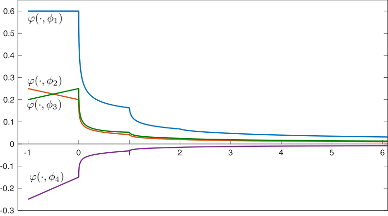
D0+0.5C​x​(t)=−5​x​(t)+0.5​x​(t−1)+x2​(t)+x3​(t−1){}^{\rm{\scriptscriptstyle C\!\!}}D^{0.5}_{0+}x(t)=-5x(t)+0.5x(t-1)+x^{2}(t)+x^{3}(t-1) (20)

is of the form (2) with a=−5a=-5, b=0.5b=0.5, f⁡(x,y)=x2+y3f(x,y)=x^{2}+y^{3}, and satisfies the assumptions of Theorem 5.1. Its trivial solution is therefore asymptotically stable.

Refer to caption
Figure 3: The solutions φ⁡(⋅,ϕi)\varphi(\cdot,\phi_{i}), i=1,2,3,4i=1,2,3,4, from Example 5.2.

Using an Adams-Bashforth-Moulton predictor-corrector scheme for fractional differential equations [2, 9], solutions φ⁡(⋅,ϕi)\varphi(\cdot,\phi_{i}) to the equation (20) are computed for the initial conditions φ⁡(t,ϕi)=ϕi​(t)\varphi(t,\phi_{i})=\phi_{i}(t) for t∈[−1,0]t\in[-1,0], i=1,2,3,4i=1,2,3,4, with the initial functions ϕi:[−1,0]→ℝ\phi_{i}\colon[-1,0]\to\mathbb{R} defined by

ϕ1​(t)\displaystyle\phi_{1}(t) =0.6,\displaystyle=0.6,
ϕ2​(t)\displaystyle\phi_{2}(t) =−0.05​t+0.2,\displaystyle=-0.05t+0.2,
ϕ3​(t)\displaystyle\phi_{3}(t) =0.05​t+0.25,\displaystyle=0.05t+0.25,
ϕ4​(t)\displaystyle\phi_{4}(t) =0.1​t−0.15,\displaystyle=0.1t-0.15,

see Figure 3.

Acknowledgement

The research of Hoang The Tuan was supported by the bilateral project between FWO Flanders and NAFOSTED Vietnam (FWO.101.2017.01). This paper was done when he visited the Center for Dynamics at TU Dresden, Germany, with the support of Deutscher Akademischer Austauschdienst (DAAD). The authors thank Ninh Van Thu and Hieu Trinh for helpful discussions.

References

  • [1] S. Abbas. Existence of solutions to fractional order ordinary and delay differential equations and applications. Electron. J. Differ. Equ., 2011 (2011), no. 9, 1–-11.
  • [2] S.B. Bhalekar, V. Daftardar-Gejji. A predictor-corrector scheme for solving nonlinear delay differential equations of fractional order. Journal of Fractional Calculus and Applications 1 (2011), 1–9.
  • [3] J. Cermak, J. Hornicek, T. Kisela. Stability regions for fractional differential systems with a time delay. Commun Nonlinear Sci Numer Simulat., 31 (2016), 108–123.
  • [4] J. Cermak, Z. Dosla, T. Kisela. Fractional differential equations with a constant delay: Stability and asymptotics of solutions. Applied Mathematics and Computation, 298 (2017), 336–350.
  • [5] N.D. Cong, H.T. Tuan. Existence, uniqueness and exponential boundedness of global solutions to delay fractional differential equations. Mediterr. J. Math., 14:193 (2017).
  • [6] N.D. Cong, T.S. Doan, H.T. Tuan. Asymptotic stability of linear fractional systems with constant coefficients and small time dependent perturbations. Vietnam Journal of Mathematics, 46 (2018), 665–680.
  • [7] N.D. Cong, H.T. Tuan. Generation of nonlocal fractional dynamical systems by fractional differential equations. Journal of Integral Equations and Applications, 29 (2017), 1–24.
  • [8] K. Diethelm. The Analysis of Fractional Differential Equations. An Application–Oriented Exposition Using Differential Operators of Caputo Type. Lecture Notes in Mathematics, 2004. Springer Verlag, Berlin, 2010.
  • [9] K. Diethelm, N.J. Ford, A.D. Freed. A predictor-corrector approach for the numerical solution of fractional differential equations. Nonlinear Dynamics, 29 (2002), 3–22.
  • [10] B.B. He, H.C. Zhou, Y.Q. Chen, C.H. Kou. Stability of fractional order systems with time delay via an integral inequality. IET Control Theory and Applications. DOI: 10.1049/iet-cta.2017.1144.
  • [11] J. Heinonen. Lectures on Lipschitz Analysis. Technical Report, University of Jyväskylä, 2005.
  • [12] D. Matignon. Stability results for fractional differential equations with applications to control processing. Computational Eng. in Sys. Appl., 2 (1996), 963–968.
  • [13] V.N. Phat, N.T. Thanh. New criteria for finite-time stability of nonlinear fractional-order delay systems: A Gronwall inequality approach. Applied Mathematics Letters, 83 (2018), 169–175.
  • [14] I. Podlubny. Fractional Differential Equations. An Introduction to Fractional Derivatives, Fractional Differential Equations, To Methods of Their Solution and Some of Their Applications. Mathematics in Science and Engineering, 198. Academic Press, Inc., San Diego, CA, 1999.
  • [15] Y. Jalilian, R. Jalilian. Existence of solution for delay fractional differential equations. Mediterr. J. Math., 20 (2013), 1731–1747.
  • [16] J. Shen, J. Lam. Stability and performance analysis for positive fractional-order systems with time-varying delays. IEEE Trans. Autom. Control., 61 (2016), no. 9, 2676–-2681.
  • [17] I.M. Stamova. On the Lyapunov theory for functional differential equations of fractional order. Proceedings of the American Mathematical Society, 144 (2016), 1581–1593.
  • [18] H.T. Tuan, H. Trinh. A linearized stability theorem for nonlinear delay fractional differential equations. To appear in IEEE Transactions on Automatic Control. DOI: 10.1109/TAC.2018.2791485.
  • [19] N. T. Thanh, H. Trinh, V. N. Phat. Stability analysis of fractional differential time-delay equations. IET Control Theory & Applications, 11 (2017), no. 7, 1006–1015.
  • [20] V. Vainikko. Which functions are fractionally differentiable? Journal of Analysis and its Applications, 35 (2016), 465–487.
  • [21] D.G. Zill, P.D. Shanahan. A First Course in Complex Analysis with Applications. Jones and Bartlett Publishers, Inc, London, UK, 2003.