Slow–fast systems and sliding on codimension 2 switching manifolds

Paulo Ricardo da Silva ^∗ and Willian Pereira Nunes ^∗ Address: ^∗ Departamento de Matemática – IBILCE–UNESP, Rua C. Colombo, 2265, CEP 15054–000 S. J. Rio Preto, São Paulo, Brazil Email address: paulo.r.silva@unesp.br Email address: willianx3@yahoo.com.br

Abstract.

In this work we consider piecewise smooth vector fields $X$ defined in $\mathbb{R}^{n}\setminus\Sigma$ , where $\Sigma$ is a self-intersecting switching manifold. A double regularization of $X$ is a 2-parameter family of smooth vector fields $X_{\varepsilon.\eta}$ , $\varepsilon,\eta>0,$ satisfying that $X_{\varepsilon,\eta}$ converges pointwise to $X$ on $\mathbb{R}^{n}\setminus\Sigma$ , when $\varepsilon,\eta\rightarrow 0$ . We define the sliding region on the non regular part of $\Sigma$ as a limit of invariant manifolds of $X_{\varepsilon.\eta}$ . Since the double regularization provides a slow–fast system, the GSP-theory (geometric singular perturbation theory) is our main tool.

Key words and phrases:

singular perturbation, non–smooth systems, invariant manifolds, Hopf bifurcation, Bogdanov-Takens bifurcation.

2010 Mathematics Subject Classification

34D15, 34C45, 34C07, 34C23, 34C25.

1. Introduction

One finds in real life and in various branches of science distinguished phenomena whose mathematical models are expressed by piecewise smooth systems and deserve a systematic analysis. However sometimes the treatment of such objects is far from the usual techniques or methodologies found in the smooth universe. A good reference for a first reading on the subject is [15].

One of the phenomena that can occur is the existence of sliding regions in the phase space. In this paper we discuss the definition of sliding when the switching manifold presents self-intersection. We begin our discussion by presenting the classical definition of sliding on a regular surface and the difficulties to extend to the general case.

Consider two smooth vector fields $X_{+},X_{-}$ defined in $\mathbb{R}^{n}=\{(x_{1},x_{2})\in\mathbb{R}\times\mathbb{R}^{n-1}\}.$ A $1$ –cross piecewise-smooth vector field is

X=\dfrac{1}{2}\left[(1+\operatorname{sgn}(x_{1}))X_{+}+(1-\operatorname{sgn}(x_{1}))X_{-})\right].

The set of discontinuity is the codimension 1 manifold $\Sigma=\{f(x_{1},x_{2})=x_{1}=0\}.$

The trajectory of $X$ by points on $\Sigma$ depends on the Lie derivative (¹¹ 1 As usual, we denote $Xf=\nabla f.X$ .), which is used to classify the points as sewing or slide:

(i)

$\Sigma_{sw}=\{x\in\Sigma:(X_{+}f.X_{-}f)(x)>0\}$ is the sewing region;
(ii)

$\Sigma_{sl}=\{x\in\Sigma:(X_{+}f.X_{-}f)(x)<0\}$ is the sliding region.

Figure 1. Sliding set

\Sigma_{sl}

(red), sewing set

\Sigma_{sw}

(blue), visible fold (green) and invisible fold (yellow).

According to Filippov’s convention [7], for $x\in\Sigma_{sl}$ , the trajectory remains in $\Sigma_{sl}$ and obeys the flow of the sliding vector field $X^{S}:\Sigma_{sl}\rightarrow\mathbb{R}^{n}$ :

X^{S}=(1-\rho)X_{+}+\rho X_{-},\quad\rho=\frac{X_{+}f}{X_{+}f-X_{-}f}.

The sliding vector field is a convex combination of $X_{+}$ and $X_{-}$ that belongs to the tangent bundle $T\Sigma$ . The Filippov’s convention [7] also provides first order exit conditions: whenever $\rho=0$ , one may expect to leave $\Sigma$ to enter in $M_{+}=f^{-1}(0,+\infty)$ with vector field $X_{+}$ , and whenever $\rho=1$ one may expected to enter in $M_{-}=f^{-1}(-\infty,0)$ with vector field $X_{-}$ . An example of first order exit point is a fold.

Our main tool for studying the sliding flow is the geometric singular perturbation theory (GSP-theory). The connection between these subjects appears when we regularize the discontinuous vector field. A regularization is a family of smooth vector fields $X_{\varepsilon}$ , with $\varepsilon\geq 0,$ satisfying that $X_{\varepsilon}$ converges uniformly to $X$ in each compact subset of $\mathbb{R}^{n}\backslash\Sigma$ when $\varepsilon\rightarrow 0$ .

The Sotomayor-Teixeira regularization [16] (ST-regularization) is based on the use of a transition function (²² 2 by definition, this is a $C^{\infty}$ function such that $\varphi(t)=-1$ for $t\leq-1$ , $\varphi(t)=1$ for $t\geq 1$ and $\varphi^{\prime}(t)>0$ for $-1<t<1$ .) $\varphi:\mathbb{R}\rightarrow\mathbb{R}$ . It is the $1$ -parameter family $X_{\varepsilon}$ given by

(1)

X_{\varepsilon}(x)=\left(\frac{1}{2}+\frac{\varphi_{\varepsilon}(x_{1})}{2}\right)X_{+}(x)+\left(\frac{1}{2}-\frac{\varphi_{\varepsilon}(x_{1})}{2}\right)X_{-}(x),

where $\varphi_{\varepsilon}(x_{1})=\varphi(x_{1}/\varepsilon)$ , for $\varepsilon>0$ .

Considering a blow-up $x_{1}\rightarrow x_{1}\varepsilon$ , the trajectories of (1) are the solutions of a slow-fast system

(2)

\varepsilon\dot{x}_{1}=\alpha(x_{1},x_{2},\varepsilon),\quad\dot{x_{2}}=\beta(x_{1},x_{2},\varepsilon).

We can apply the GSP-theory to get information about its phase portrait for $\varepsilon\sim 0$ (see for instance [2, 9, 10, 11, 12]). On the paper [10] one has the proof that the reduced dynamics on the critical manifold $\mathcal{S}_{0}=\{\alpha(x_{1},x_{2},0)=0\}$ is equivalent to the dynamics of sliding vector field on $\Sigma_{sl}$ . Consequently $\Sigma_{sl}$ is the limit of invariant manifolds $\mathcal{S}_{\varepsilon}$ of $X_{\varepsilon}$ . We can roughly say that the Filippov’s approach and the singular perturbation approach provide the same description of the sliding vector field on $\Sigma.$ However, when the discontinuity occurs in a set $\Sigma\subseteq M$ with codimension greater than $1$ , the sliding region can not be defined via Filippov’s convention. The main goal of this paper is to study slide on $\Sigma$ with codimension $2$ . We refer [1, 3, 4, 5, 13] for related problems and for an introduction to the subject.

1.1. Set of discontinuity $\Sigma\subseteq\mathbb{R}^{n}$ with codimension 2 points.

Consider now four smooth vector fields $X_{++},X_{-+},X_{--},X_{+-}$ defined in $\mathbb{R}^{n}=\{(x_{1},x_{2},x_{3})\in\mathbb{R}\times\mathbb{R}\times\mathbb{R}^{n-2}\}$ and the $2$ –cross piecewise-smooth vector field

(3)

X=\dfrac{1}{4}\left[aX_{++}+bX_{+-}+cX_{-+}+dX_{--}\right]

where

a=(1+\operatorname{sgn}(x_{1}))(1+\operatorname{sgn}(x_{2})),\quad b=(1+\operatorname{sgn}(x_{1}))(1-\operatorname{sgn}(x_{2})),

c=(1-\operatorname{sgn}(x_{1}))(1+\operatorname{sgn}(x_{2})),\quad d=(1-\operatorname{sgn}(x_{1}))(1-\operatorname{sgn}(x_{2})).

Denote $\Sigma_{1}=\{x_{1}=0\}\subset\mathbb{R}^{n}$ and $\Sigma_{2}=\{x_{2}=0\}\subset\mathbb{R}^{n}$ . The set $\Sigma=\Sigma_{1}\cup\Sigma_{2}$ is the switching manifold and the phase space is divided into four regions, denoted by

	$\displaystyle M_{++}:\ x_{1}>0,x_{2}>0,$	$\displaystyle M_{+-}:\ x_{1}>0,x_{2}<0,$
	$\displaystyle M_{--}:\ x_{1}<0,x_{2}<0,$	$\displaystyle M_{-+}:\ x_{1}<0,x_{2}>0.$

We also use the following notation

\Sigma_{1}^{\pm}=\left\{x_{1}=0,x_{2}\gtrless 0\right\},\Sigma_{2}^{\pm}=\left\{x_{2}=0,x_{1}\gtrless 0\right\}.

The codimension 2 switching set is $\Sigma_{00}=\left\{x_{1}=x_{2}=0\right\}.$ Inspired in the regular case, we try to find a sliding vector field as a convex combination of $X_{++},X_{-+},X_{--}$ and $X_{+-}$ :

(4)

X\in\left\{\sum_{s\in\{-,+\}^{2}}\lambda_{s}X_{s},\quad\sum_{s\in\{-,+\}^{2}}\lambda_{s}=1\right\},\quad X.x_{i}=0,i=1,2.

Clearly it is an indeterminate system. Thus the requirement of $X$ being tangent to $\Sigma_{1}$ and $\Sigma_{2}$ is not sufficient to characterize a convex combination of $X_{++},X_{-+},X_{--}$ and $X_{+-}$ .

In [14] we propose a new definition for sliding and sewing, linked to the regularization considered. Our definition coincides with the definition of Filippov in the regular case. Thus, we can say that our definition generalizes the previous one.

Let $\varphi:\mathbb{R}\longrightarrow\mathbb{R}$ be a transition function. The double regularization is

X_{\varepsilon,\eta}(\textbf{x})=\frac{1}{4}\left(\sum_{s}\left(1+s_{1}\varphi\left(\frac{x_{1}}{\varepsilon}\right)\right)\left(1+s_{2}\varphi\left(\frac{x_{2}}{\eta}\right)\right)X_{s}(\textbf{x})\right)

where $s=(s_{1},s_{2})\in\{-,+\}^{2}$ .

Definition 1.1.

(Slide depending on regularization $X_{\varepsilon,\eta}$ .) We say that $p\in\Sigma_{00}$ is a sliding point of (3) if there exist an open neighborhood $U\subset\mathbb{R}^{n}$ of $p$ and a family of smooth manifolds $S_{\varepsilon,\eta}\subset U$ defined for all $\varepsilon,\eta>0$ such that:

•

For each $\varepsilon,\eta$ , $S_{\varepsilon,\eta}$ is invariant by the restriction of $X_{\varepsilon,\eta}$ to $U$ .
•

For each compact subset $K\subset U$ , the sequence $S_{{\varepsilon},\eta}\cap K$ converges to $\Sigma_{00}\cap K$ when $(\varepsilon,\eta)\rightarrow(0,0)$ in some given Hausdorff metric $d_{H}$ on compact sets of $\mathbb{R}^{n}$ .

We remark that the sliding condition is open, that is, if $p\in\Sigma_{00}$ is a sliding point then there exists an open neighborhood $I\subset\Sigma_{00}$ such that any $q\in I$ is a sliding point.

Briefly, we list below the results we have proved in this article. When considering $(\varepsilon,\eta)\rightarrow(0,0)$ we can obtain different limit situations depending on the iteration between the parameters. We call regularization curve a path $\psi(\varepsilon,\eta)=0,$ with $\psi(0,0)=0$ , in the parameter space $(\varepsilon,\eta)$ .

•

(Regularization curve $\eta=k\varepsilon$ ) If $\Sigma_{00}$ is the codimension 2 switching manifold then the sliding region in $\Sigma_{00}$ (linked to $X_{\varepsilon,k\varepsilon}$ ) is characterized by the signal of a smooth function. See Theorem 3.1.
•

(General regularization curve) If $\Sigma_{00}$ is the codimension 2 switching manifold and the singular points of $X_{s}$ , $s\in\{-,+\}^{2}$ , are not in $\Sigma$ then the sliding region in $\Sigma_{00}$ (linked to $X_{\varepsilon,\eta}$ ) depends on the interactions between the parameters $\varepsilon$ and $\eta$ . See Theorems 4.1 and 4.2.

Figure 2. A codimension 2 switching manifold

\Sigma

and double regularization.

The paper is organized as follows. In Section 2 we give preliminary definitions and remember the main results of GSP-theory. In Section 3 we consider a regularizing curve of the kind $\eta=k\varepsilon$ , $k>0$ . Combining blowing-up technique and Fenichel’s theory we give sufficient conditions for identifying the sliding region. In Section 4 we state and prove the main result, which consists in conditions for identifying the sliding using the parameters of the double regularization. In Section 5, we study a class of planar quadratic system, that is useful to determine the sliding regions. In Section 6 some examples are presented to illustrate the main results.

2. Basic Tools

This section is dedicated to presenting preliminary results that will be necessary to prove our main results.

2.1. Singular Perturbation Tools

Let $\mathcal{U}\subseteq\mathbb{R}^{n+m}$ be an open subset. A singular perturbation problem in $\mathcal{U}$ is a differential system which can be written like

(5)

\displaystyle\varepsilon\dot{x}_{1}=\alpha(x_{1},x_{2},\varepsilon),\quad\dot{x}_{2}=\beta(x_{1},x_{2},\varepsilon),

with $\alpha,\beta$ smooth functions, $\varepsilon\in(-\varepsilon_{0},\varepsilon_{0})$ , $\varepsilon_{0}>0$ small and $(x_{1},x_{2})\in\mathcal{U}\subseteq\mathbb{R}^{n}\times\mathbb{R}^{m}$ . Equivalently, after the time rescaling $\tau=t/\varepsilon$ , system (5) becomes

(6)

\displaystyle x_{1}^{\prime}=\alpha(x_{1},x_{2},\varepsilon),\quad x^{\prime}_{2}=\varepsilon\beta(x_{1},x_{2},\varepsilon).

The systems (5) and (6) are called slow system and fast system, respectively. By setting $\varepsilon=0$ in (5) and (6), we obtain two different limit problems, the reduced problem

(7)

\displaystyle\dot{x}_{2}=\beta(x_{1},x_{2},0),\quad 0=\alpha(x_{1},x_{2},0),

and the layer problem

(8)

\displaystyle x^{\prime}_{1}=\alpha(x_{1},x_{2},0),\quad x^{\prime}_{2}=0.

Under adequate assumptions, $\alpha(x_{1},x_{2},0)=0$ defines a manifold $\mathcal{S}$ , that will be called critical manifold, on which (7) defines a dynamical system. But at the same time $\mathcal{S}$ is the set of equilibrium points of (8). So, appropriately combining results on the dynamics of these two limiting problems, we obtain results on the dynamics of the singularly perturbed problem, for $\varepsilon$ sufficiently small.

Consider system (6) suplemented by $\varepsilon^{\prime}=0$ ,

(9)

\displaystyle x^{\prime}_{1}=\alpha(x_{1},x_{2}\varepsilon),\quad x^{\prime}_{2}=\varepsilon\beta(x_{1},x_{2}\varepsilon),\quad\varepsilon^{\prime}=0,

which is defined in $\mathcal{U}\times(-\varepsilon_{0},\varepsilon_{0})$ . The vector field associated to (9) will be denoted by

(10)

X(x_{1},x_{2},\varepsilon)=(\alpha(x_{1},x_{2},\varepsilon),\varepsilon\beta(x_{1},x_{2},\varepsilon),0),

with $(x_{1},x_{2},\varepsilon)\in\mathcal{U}\times(-\varepsilon_{0},\varepsilon_{0})$ . By calculating the eigenvalues of $LX(x_{1},x_{2},0)$ , with $(x_{1},x_{2})\in\mathcal{S}$ , we have that $\lambda=0$ is a trivial eigenvalue of algebraic multiplicity $m+1$ . The remaining eigenvalues are called nontrivial eigenvalues. We denote the numbers of nontrivial eigenvalues in the left half plane, in the imaginary axis and in the right half plane by $k^{s}$ , $k^{c}$ and $k^{u}$ , respectively.

Let $\mathcal{S}_{r}\subset\mathcal{S}$ be the open set where the nontrivial eigenvalues are nonzero. The manifold $\mathcal{S}_{r}$ can be characterized as

\mathcal{S}_{r}=\{(x_{1},x_{2})\in\mathcal{S}:\text{rank\ }D_{x_{1}}\alpha(x_{1},x_{2},0)=n\}.

$\mathcal{S}_{r}$ can be parametrized, locally, by solving the equation $\alpha(x_{1},x_{2},0)=0$ , using the implicit function theorem. Let $\mathcal{S}_{h}\subset\mathcal{S}_{r}$ be the open set where all the nontrivial eigenvalues have nonzero real part, i.e, compact sets $K\subset\mathcal{S}_{h}$ are normally hyperbolic invariant manifolds of (8).

Next theorem is a classical result due to Fenichel, and its proof can be founded in [6, 17].

Theorem 2.1.

Let $X(x_{1},x_{2},\varepsilon)$ , $\varepsilon\in(-\varepsilon_{0},\varepsilon_{0})$ be the family of smooth vector fields on $\mathcal{U}$ given by (10) and $\mathcal{S}$ its slow manifold. Let $\mathcal{N}\subset\mathcal{S}_{h}$ be a $j$ -dimensional compact invariant manifold of the reduced vector field (7), with a $j+j^{s}$ -dimensional local stable manifold $W^{s}$ and a $j+j^{u}$ -dimensional local unstable manifold $W^{u}$ .

i-)

There exist $\varepsilon_{1}>0$ and a family of smooth manifolds $\mathcal{N}_{\varepsilon}$ with $\varepsilon\in(0,\varepsilon_{1})$ such that $\mathcal{N}_{0}=\mathcal{N}$ and $\mathcal{N}_{\varepsilon}$ is an invariant manifold of $X(x_{1},x_{2},\varepsilon)$ ;
ii-)

There are a family of smooth manifolds $(j+j^{s}+k^{s})$ -dimensional $\mathcal{N}_{\varepsilon}^{s}$ with $\varepsilon\in(0,\varepsilon_{1})$ and family of smooth manifolds $(j+j^{u}+k^{u})$ -dimensional $\mathcal{N}_{\varepsilon}^{u}$ with $\varepsilon\in(0,\varepsilon_{1})$ such that the manifolds $\mathcal{N}_{\varepsilon}^{s}$ and $\mathcal{N}_{\varepsilon}^{u}$ are, locally, stable and unstable manifolds of $\mathcal{N}_{\varepsilon}$ .

2.2. Sliding region depending on the regularization

In this section, we introduce some concepts for piecewise smooth systems.

Definition 2.1.

Let $0<m\leq n$ be integers.

a.

The subset $\Sigma\subset\mathbb{R}^{n}$ given by $\Sigma=\left\{\prod_{k=1}^{m}x_{k}=0\right\}$ is called a $m$ -cross.
b.

A $m$ -cross piecewise-smooth vector field defined on $\mathbb{R}^{n}$ is a vector field of the kind

$X=\dfrac{1}{2^{m}}\sum_{s}L_{s}(\operatorname{sgn}(x))X_{s}$

where $\{X_{s}\}$ is a collection of $2^{m}$ smooth vector fields, $s=(s_{1},...,s_{m})\in\{-,+\}^{m}$ , $\operatorname{sgn}(x)=(\operatorname{sgn}(x_{1}),\cdots,\operatorname{sgn}(x_{m}))\in\{-,+\}^{m}$ and

$L_{s}(y)=\frac{1}{2^{m}}\prod_{k=1}^{m}(1+s_{k}y_{k}).$

Thus a $1$ –cross piecewise-smooth vector field defined on $\mathbb{R}^{2}$ is

X=\dfrac{1}{2}\left[(1+\operatorname{sgn}(x_{1}))X_{+}+(1-\operatorname{sgn}(x_{1}))X_{-})\right]

and a $2$ –cross piecewise-smooth vector field defined on $\mathbb{R}^{3}$ is

X=\dfrac{1}{4}\left[aX_{++}+bX_{+-}+cX_{-+}+dX_{--}\right]

where

a=(1+\operatorname{sgn}(x_{1}))(1+\operatorname{sgn}(x_{2})),\quad b=(1+\operatorname{sgn}(x_{1}))(1-\operatorname{sgn}(x_{2})),

c=(1-\operatorname{sgn}(x_{1}))(1+\operatorname{sgn}(x_{2})),\quad d=(1-\operatorname{sgn}(x_{1}))(1-\operatorname{sgn}(x_{2})).

Refer to caption — Figure 3. Possible $m$ -cross on $\mathbb{R}^{2}$ and on $\mathbb{R}^{3}$ .

Let $\varphi:\mathbb{R}\longrightarrow\mathbb{R}$ be a monotonic transition function. We are going to use a particular kind of regularization, which is induced by $\varphi$ .

Definition 2.2.

Given a transition function $\varphi$ , the regularization of $m$ -cross piecewise-smooth vector field $X$ , is the family of smooth vector fields

(11)

X_{\varepsilon}^{\varphi}=\frac{1}{2^{m}}\sum_{s}L_{s}\left(\varphi\left(\frac{x_{1}}{\varepsilon_{1}}\right),\cdots,\varphi\left(\frac{x_{m}}{\varepsilon_{m}}\right)\right)X_{s},

with $s\in\{-,+\}^{m}$ and $\varepsilon\in(\mathbb{R}_{+})^{m}$ .

Note that induced regularization of a $1$ -cross is the well known Sotomayor-Teixeira regularization.

Denote

\Sigma_{s}=\{\operatorname{sgn}_{0}(x_{1})=s_{1},\cdots,\operatorname{sgn}_{0}(x_{n})=s_{n}\},

where $\operatorname{sgn}_{0}(x)$ is the sign function extended to $0$ by $\operatorname{sgn}_{0}(0)=0$ . Consider the stratification of $\mathbb{R}^{n}=\bigcup_{s}\Sigma_{s},$ where the union is taken over all sign vectors $s=(s_{1},\cdots,s_{m})\in\{0,-,+\}^{m}$ . Each $\Sigma_{s}$ is a submanifold of codimension equal to the number $z(s)$ of zeros in the sign vector $s$ . Notice that this induces a stratification of the $m$ -cross

\Sigma=\bigcup_{z(s)>0}\Sigma_{s},

where the union is taken over all sign vectors $s$ such that $z(s)>0$ .

A regularizing curve is a continuous parametrized curve $\varepsilon(\mu)$ in the parameter space $(\mathbb{R}_{+})^{m}$ such as $\displaystyle\lim_{\mu\rightarrow 0}\varepsilon(\mu)=0$ .

Definition 2.3.

Let $\Sigma_{s}$ be one of the strata of $\Sigma$ . We say that a regularizing curve $\varepsilon(\mu)$ produces a sliding along $\Sigma_{s}$ if there exists a smooth manifold $S$ of codimension $z(s)$ in product space $(\mu,x)\in\mathbb{R}_{\geq 0}\times\mathbb{R}^{n}$ such that:

i.

$S\cap\{\mu=0\}=\Sigma_{s}$ ;
ii.

For each $\mu_{0}>0$ , $S_{\mu_{0}}=S\cap\{\mu=\mu_{0}\}$ is an invariant manifold for the induced vector field $X_{\varepsilon(\mu_{0})}^{\varphi}$ .

3. $2$ -cross and regularization curve $(\varepsilon,k\varepsilon)$

In this section we study the sliding associated with $2$ -cross piecewise-smooth vector field $X$ on $\mathbb{R}^{n}$ with $n>2$ . Without loss of generality we assume that $n=3$ and

(12)

X=\frac{1}{4}\sum_{s\in\{-,+\}^{2}}L_{s}(\operatorname{sgn}(\textbf{x}))X_{s}

where $X_{s}(\textbf{x})=(f_{s}(\textbf{x}),g_{s}(\textbf{x}),h_{s}(\textbf{x}))$ is smooth and $\textbf{x}=(x_{1},x_{2},x_{3})$ .

Let $\varphi:\mathbb{R}\longrightarrow\mathbb{R}$ be a transition function. Consider the regularization

(13)

X_{\varepsilon,\eta}(\textbf{x})=\frac{1}{4}\left(\sum_{s\in\{-,+\}^{2}}\left(1+s_{1}\varphi\left(\frac{x_{1}}{\varepsilon}\right)\right)\left(1+s_{2}\varphi\left(\frac{x_{2}}{\eta}\right)\right)X_{s}(\textbf{x})\right)

and its corresponding differential system

(14)

\displaystyle\begin{split}x_{1}^{\prime}&=\frac{1}{4}\left(\sum_{s\in\{-,+\}^{2}}\left(1+s_{1}\varphi\left(\frac{x_{1}}{\varepsilon}\right)\right)\left(1+s_{2}\varphi\left(\frac{x_{2}}{\eta}\right)\right)f_{s}(\textbf{x})\right),\\ x_{2}^{\prime}&=\frac{1}{4}\left(\sum_{s\in\{-,+\}^{2}}\left(1+s_{1}\varphi\left(\frac{x_{1}}{\varepsilon}\right)\right)\left(1+s_{2}\varphi\left(\frac{x_{2}}{\eta}\right)\right)g_{s}(\textbf{x})\right),\\ x_{3}^{\prime}&=\frac{1}{4}\left(\sum_{s\in\{-,+\}^{2}}\left(1+s_{1}\varphi\left(\frac{x_{1}}{\varepsilon}\right)\right)\left(1+s_{2}\varphi\left(\frac{x_{2}}{\eta}\right)\right)h_{s}(\textbf{x})\right).\end{split}

The sliding region on $\Sigma_{s}$ , for $s=(s_{1},s_{2})\neq(0,0)$ , has been extensively studied and agree with the Filippov’s convention. However, on $\Sigma_{00}$ the classical approach does not apply, as seen in Section 1. Thus, we adopt the definition of sliding region introduced in the previous section.

First of all, we consider the double regularization with only one parameter $\varepsilon$ , that is, we choose a regularization curve of the kind $(\varepsilon,K\varepsilon)$ , with $K>0$ . Thus, in system (14) we replace $\eta$ by $K\varepsilon$ .

Theorem 3.1.

Consider the $2$ -cross piecewise smooth vector field (12). There exists a smooth function $D(x_{3})$ satisfying that if $D(x_{3})\neq 0$ then $(0,0,x_{3})\in\Sigma_{00}$ is a sliding point according to regularization (13), with $\eta=K\varepsilon$ .

Proof.

Consider the regularized system (14). The blow-up $x_{1}\rightarrow\varepsilon x_{1}$ and $x_{2}\rightarrow K\varepsilon x_{2}$ , provides

(15)

{x}_{1}^{\prime}=X_{1}({\textbf{x}},\varepsilon),\quad{x}_{2}^{\prime}=X_{2}({\textbf{x}},\varepsilon)\quad x_{3}^{\prime}=X_{3}({\textbf{x}},\varepsilon),

where

\displaystyle\begin{split}X_{1}({\textbf{x}},\varepsilon)&=\frac{1}{4\varepsilon}\left(\sum_{s\in\{-,+\}^{2}}\left(1+s_{1}\varphi\left({x}_{1}\right)\right)\left(1+s_{2}\varphi\left({x}_{2}\right)\right)f_{s}(\varepsilon{x}_{1},K\varepsilon{x}_{2},x_{3})\right),\\ X_{2}({\textbf{x}},\varepsilon)&=\frac{1}{4K\varepsilon}\left(\sum_{s\in\{-,+\}^{2}}\left(1+s_{1}\varphi\left({x}_{1}\right)\right)\left(1+s_{2}\varphi\left({x}_{2}\right)\right)g_{s}(\varepsilon{x}_{1},K\varepsilon{x}_{2},x_{3})\right),\\ X_{3}({\textbf{x}},\varepsilon)&=\frac{1}{4}\left(\sum_{s\in\{-,+\}^{2}}\left(1+s_{1}\varphi\left({x}_{1}\right)\right)\left(1+s_{2}\varphi\left({x}_{2}\right)\right)h_{s}(\varepsilon{x}_{1},K\varepsilon{x}_{2},x_{3})\right),\end{split}

with ${\textbf{x}}=({x}_{1},{x}_{2},x_{3})$ . System (15) is the slow system and the corresponding vector field is denoted by $X_{\varepsilon}({\textbf{x}},\varepsilon)=(X_{1}({\textbf{x}},\varepsilon),X_{2}({\textbf{x}},\varepsilon),X_{3}({\textbf{x}},\varepsilon))$ .

For ${\textbf{x}}_{0}\in S=\{X_{1}({\textbf{x}},0)=0\}\cap\{X_{2}({\textbf{x}},0)=0\}$ denote $D_{0}$ the matrix of

D_{({x}_{1},{x}_{2})}\left(X_{1},X_{2}\right)({\textbf{x}}_{0},0).

We will prove that $D(x_{3})=\operatorname{tr}(D_{0}).\det(D_{0})\neq 0$ implies $(0,0,x_{3})$ to be a sliding point of $X$ .

For $\varepsilon=0$ , $S$ is the slow manifold of system (15). Let $S_{r}\subset S$ be the open subset of $S$ given by $S_{r}=\{{\textbf{x}}\in S:\text{rank\ }D_{({x}_{1},{x}_{2})}\left(X_{1},X_{2}\right)({\textbf{x}},0)=2\}.$ The matrix $D_{0}$ is given by

(16)

\left[\begin{array}[]{rrrr}\displaystyle\frac{\partial X_{1}({\textbf{x}}_{0},0)}{\partial{x}_{1}}&\displaystyle\frac{\partial X_{1}({\textbf{x}}_{0},0)}{\partial{x}_{2}}\\ \\ \displaystyle\frac{\partial X_{2}({\textbf{x}}_{0},0)}{\partial{x}_{1}}&\displaystyle\frac{\partial X_{2}({\textbf{x}}_{0},0)}{\partial{x}_{2}}\end{array}\right].

The hypothesis implies that the rank of $D_{0}$ is $2$ and the eigenvalues of $D_{0}$ have nonzero real part. In other words, ${\textbf{x}}_{0}\in S_{h}\subset S_{r}$ . Since $S_{h}$ is a open set there exists a neighborhood $V\ni{\textbf{x}}_{0}$ such that $\bar{V}\subset S_{h}$ . Using the Theorem 2.1, there exists a $C^{r-1}$ family of manifolds ${V}_{\varepsilon}$ with $\varepsilon\in(0,\varepsilon_{1})$ such that ${V}_{0}={V}$ and ${V}_{\varepsilon}$ is an invariant manifold $X(\textbf{x},\varepsilon)$ , proving that $(0,0,x_{3})$ is a sliding point for $X$ .

∎

Example 1.

Let $X$ be a $2$ -cross piecewise-smooth vector field defined on $\mathbb{R}^{3}$ , given by $X(x,y,z)=X_{\pm\pm}(x,y,z)$ where

\displaystyle\begin{split}X_{++}=&\left(-1+x^{2},-1+y^{2},z\right)\ \ &X_{+-}=&\left(-1+xy,1-zy,z\right)\\ X_{--}=&\left(1,1+z^{2},z\right)\ \ &X_{-+}=&\left(1+x+z,-1,z\right),\end{split}

Consider the regularization of $X$ and the directional blow-up $x\rightarrow\varepsilon x$ , $y\rightarrow\varepsilon y$ . System (15) is

(17)

\varepsilon x^{\prime}=X_{1}(\textbf{x});\quad\varepsilon y^{\prime}=X_{2}(\textbf{x});\quad z^{\prime}=X_{3}(\textbf{x}),

$\textbf{x}=(x,y,z)$ ,where

X_{1}=\left(x^{3}-zx-3x+z+y(x^{3}+x^{2}-xz+2x+z)+y^{2}(-x^{2}-x)\right)/4

X_{2}=\left(-xz^{2}+z^{2}+y(xz^{2}-xz-z^{2}-z-4)+y^{2}(xz+x+z+1)+y^{3}(x+1)\right)/4

and $X_{3}(\textbf{x})=z$ . We are going to check if $p=(0,0,0)\in\Sigma_{00}$ is a sliding point. The function $D(z)$ is given by

D(z)=\left(-{z}^{2}-2\,z-7\right)\left(2\,{z}^{3}+4\,{z}^{2}+7\,z+12\right).

Since $D(p)=-84\neq 0$ , $p$ is a sliding point.

4. Sliding depending of the regularization curve

In this section we study the sliding associated with $2$ -cross piecewise-smooth vector fields generated by smooth vector fields $F_{s}:\mathbb{R}^{3}\rightarrow\mathbb{R}^{3},s\in\{-,+\}^{2}$ satisfying that $F_{s}(0,0,0)\neq 0$ . Initially we consider constant vector fields $X_{s},s\in\{-,+\}^{2}$ defined in $\mathbb{R}^{3}$ and then we extend our result to the general case via tubular flow.

Assume that $X_{s}=(a_{s},b_{s},1)$ with $a_{s},b_{s}\in\mathbb{R}$ , $s=(s_{1},s_{2})\in\{-,+\}^{2}$ . Given a transition function $\varphi:\mathbb{R}\longrightarrow\mathbb{R}$ , consider the regularization

(18)

X_{\varepsilon,\eta}(\textbf{x})=\frac{1}{4}\left(\sum_{s}\left(1+s_{1}\varphi\left(\frac{x_{1}}{\varepsilon}\right)\right)\left(1+s_{2}\varphi\left(\frac{x_{2}}{\eta}\right)\right)X_{s}(\textbf{x})\right),

with $\textbf{x}=(x_{1},x_{2},x_{3})$ . Here $(\varepsilon,\eta)$ is an arbitrary regularization curve. First of all take the directional blow-up $x_{1}\rightarrow\varepsilon x_{1}$ and $x_{2}\rightarrow\eta x_{2}$ . The corresponding differential system is

(19)

\left\{\begin{aligned} {x}_{1}^{\prime}&=\frac{1}{\varepsilon}\sum_{s}\left(1+s_{1}\varphi({x}_{1})\right)\left(1+s_{2}\varphi({x}_{2})\right)a_{s},\\ {x}_{2}^{\prime}&=\frac{1}{\eta}\sum_{s}\left(1+s_{1}\varphi({x}_{1})\right)\left(1+s_{2}\varphi({x}_{2})\right)b_{s},\\ x_{3}^{\prime}&=1,\quad\varepsilon^{\prime}=0,\quad\eta^{\prime}=0.\\ \end{aligned}\right.

The flow of system (19) depends essentially on the first two rows. We refer to these two lines as ${x}_{1}{x}_{2}$ –system.

(20)

\left\{\begin{aligned} {x}_{1}^{\prime}&=\frac{1}{\varepsilon}\sum_{s}\left(1+s_{1}\varphi({x}_{1})\right)\left(1+s_{2}\varphi({x}_{2})\right)a_{s},\\ {x}_{2}^{\prime}&=\frac{1}{\eta}\sum_{s}\left(1+s_{1}\varphi({x}_{1})\right)\left(1+s_{2}\varphi({x}_{2})\right)b_{s}.\end{aligned}\right.

Analyzing the dynamics of (20), we obtain conditions to define the sliding of system $X$ . Near $(0,0)$ we have $\varphi({x}_{1})\approx{x}_{1}$ and $\varphi({x}_{2})\approx{x}_{2}$ . Using this equivalence, with a time reescaling $t=\varepsilon\tau$ , the system (20) is equivalent to

(21)

\left\{\begin{aligned} \dot{{x}}_{1}&=\sum_{s}\left(1+s_{1}{x}_{1}\right)\left(1+s_{2}{x}_{2}\right)a_{s},\\ \dot{{x}}_{2}&=\frac{\varepsilon}{\eta}\sum_{s}\left(1+s_{1}{x}_{1}\right)\left(1+s_{2}{x}_{2}\right)b_{s}.\end{aligned}\right.

If $\lambda_{1}=(a_{++}-a_{-+}-a_{+-}+a_{--})/4\neq 0$ and $\lambda_{2}=(b_{++}-b_{-+}-b_{+-}+b_{--})/4\neq 0$ then system (21) is quadratic and it can be written as

(22)

\left\{\begin{aligned} \dot{{x}}_{1}&=\lambda_{1}({x}_{1}-\alpha_{1})({x}_{2}-\beta_{1})-\delta_{1},\\ \dot{{x}}_{2}&=\frac{\varepsilon}{\eta}\lambda_{2}({x}_{1}-\alpha_{2})({x}_{2}-\beta_{2})-\delta_{2},\end{aligned}\right.

where $\alpha_{1}=-(a_{++}+a_{-+}-a_{+-}-a_{--})/\lambda_{1}$ , $\beta_{1}=-(a_{++}-a_{-+}+a_{+-}-a_{--})/\lambda_{1}$ and $\delta_{1}=(\lambda_{1}\alpha_{1}\beta_{1}-\left(a_{++}+a_{-+}+a_{+-}+a_{--}\right))/4$ . For $\alpha_{2},\beta_{2}$ e $\delta_{2}$ , the expressions are the same but changing $a_{i}$ by $b_{i}$ .

Proposition 4.1.

If system (22) has two equilibria, then only one of them is a saddle point.

Proof.

The linearization of system (22) is

L({x}_{1},{x}_{2})=\left[\begin{array}[]{cc}\lambda_{1}\,\left({x}_{2}-\beta_{1}\right)&\lambda_{1}\,\left({x}_{1}-\alpha_{1}\right)\\ \vskip 6.0pt plus 2.0pt minus 2.0pt\cr{\displaystyle\frac{\varepsilon\,\lambda_{2}\,\left({x}_{2}-\beta_{2}\right)}{\eta}}&{\displaystyle\frac{\varepsilon\,\lambda_{2}\,\left({x}_{1}-\alpha_{2}\right)}{\eta}}\end{array}\right]

and it has determinant given by

\det({x}_{1},{x}_{2})=-{\frac{\lambda_{1}\,\varepsilon\,\lambda_{2}\,\left(\beta_{1}\,{x}_{1}-\beta_{1}\,\alpha_{2}-{x}_{1}\beta_{2}+\alpha_{1}\,\beta_{2}-\alpha_{1}\,{x}_{2}+{x}_{2}\alpha_{2}\right)}{\eta}}.

If system (22) has two distinct equilibra $P_{1},P_{2}$ , we have that $\alpha_{1}\neq\alpha_{2}$ and $\beta_{1}\neq\beta_{2}$ . So $\det({x}_{1},{x}_{2})=0$ defines a straight line passing through the points $(\alpha_{1},\beta_{1})$ and $(\alpha_{2},\beta_{2})$ . Note that, the ratio between the parameters does not affect the straight line determined by $\det({x}_{1},{x}_{2})=0$ , for any $\varepsilon,\eta$ . So, the intersection $\dot{{x}}_{1}=0$ and $\dot{{x}}_{2}=0$ , which give us the equilibria, occurs on opposite sides of $\det({x}_{1},{x}_{2})=0$ , that is, $\det(P_{1})\det(P_{2})<0$ , proving that one of the points is a saddle. ∎

Applying a translation ${x}_{1}-\alpha_{1}$ , ${x}_{2}-\beta_{1}$ , and a time reescaling $\tau_{1}=\tau/\lambda_{1}$ on (22) we get

(23)

\left\{\begin{aligned} \dot{{x}}_{1}&={x}_{1}{x}_{2}-\delta_{1}\\ \dot{{x}}_{2}&=\frac{\varepsilon}{\eta}C({x}_{1}-{\alpha}_{2})({x}_{2}-{\beta}_{2})-\delta_{2},\end{aligned}\right.

where $C=\lambda_{2}/\lambda_{1}$ and possibly different constants $\alpha_{1},\alpha_{2}$ .

Proposition 4.2.

Let $X$ be the vector field (23) having two equilibria $P,Q$ where $P=({x_{1}},{x_{2}})$ denotes the non-saddle equilibrium with ${x_{1}}\neq 0$ .

i.

If $\frac{\varepsilon}{\eta}\rightarrow k$ , as $\varepsilon,\eta\rightarrow 0$ , with $k>0$ , then the nature of $P$ and $Q$ do not change, for any $\varepsilon,\eta$ ;
ii.

If $\frac{\varepsilon}{\eta}\rightarrow 0$ or $\frac{\varepsilon}{\eta}\rightarrow\infty$ as $\varepsilon,\eta\rightarrow 0$ , then $P$ is asymptotically stable or asymptotically unstable. Moreover, if $P$ is asymptotically stable (unstable) for $\frac{\varepsilon}{\eta}\rightarrow 0$ then it is asymptotically unstable (stable) for $\frac{\varepsilon}{\eta}\rightarrow\infty.$

Proof.

The linearization of the system (23) depending of ${x}_{1}$ and ${x}_{2}$ is

J=\left[\begin{array}[]{cc}{x}_{2}&{x}_{1}\\ \vskip 6.0pt plus 2.0pt minus 2.0pt\cr\displaystyle\frac{\varepsilon C({x}_{2}-{\alpha}_{2})}{\eta}&\displaystyle\frac{\varepsilon C({x}_{1}-{\beta}_{2})}{\eta}\end{array}\right]

Note that the trace and the determinant are given, respectively, by

\text{Tr}({x}_{1},{x}_{2})={x}_{2}+{\frac{\varepsilon\,C\left({x}_{1}-{\alpha}_{2}\right)}{\eta}}\text{\ and \ }\det({x}_{1},{x}_{2})=-{\frac{\varepsilon\,C\left({\beta}_{2}{x}_{1}-{\alpha}_{2}{x}_{2}\right)}{\eta}}.

Tr $({x}_{1},{x}_{2})=0$ and $\det({x}_{1},{x}_{2})=0$ , define two straight lines in the plane ${x}_{1}{x}_{2}$ , which we denote, respectively, by $r_{1},r_{2}$ . The line $r_{2}$ is independent of the parameters $\varepsilon$ and $\eta$ , but the inclination of line $r_{1}$ depends of the quotient $\varepsilon/\eta$ . By Proposition 4.1 one of these equillibrium points is a saddle and the other depends of the line $r_{1}$ . Assuming i, the inclination of $r_{1}$ does not change for $\varepsilon,\eta\rightarrow 0$ , that is, the nature of $P,Q$ does not change. Now, assume ii with $\varepsilon/\eta\rightarrow 0$ . In this case $r_{1}$ tends to $y=0$ , and the stability of $P$ depends on its position in relation to $r_{1}$ and $r_{2}$ and remains for $\varepsilon$ and $\eta$ sufficiently small. If $\varepsilon/\eta\rightarrow\infty$ the position of $P$ does not change, but $r_{1}$ tends to $y={\alpha}_{2}$ , which implies that for sufficiently small values of $\varepsilon$ and $\eta$ , the stability is opposite, proving the theorem.

∎

Observe that, the proof of Proposition 4.2,i, could be obtained using the Theorem 2.1. For only one equilibrium point, the proof is the same.

Theorem 4.1.

Let $X$ be a $2$ -cross piecewise-smooth constant vector field defined in $\mathbb{R}^{3}$ and generated by $X_{s}=(a_{s},b_{s},1)$ with $a_{s},b_{s}\in\mathbb{R}$ , $s=(s_{1},s_{2})\in\{-,+\}^{2}$ . Consider the regularization $X_{\varepsilon,\eta}$ given by (18) and apply the blow up (19). Assume that the equilibria points of the ${x}_{1}{x}_{2}$ –system (20) are localized at $(-1,1)^{2}$ .

i.

If ${x}_{1}{x}_{2}$ –system has two equilibria, then every point in $\Sigma_{00}$ is a sliding point of $X$ , for any $\varepsilon,\eta$ .
ii.

If ${x}_{1}{x}_{2}$ –system has only one equilibrium and it is asymptotically stable or unstable when $\varepsilon,\eta\rightarrow 0$ , then every point in $\Sigma_{00}$ is a sliding point of $X$ .

Proof.

Let’s assume first that we have two equilibria for the ${x}_{1}{x}_{2}$ –system. According to the Proposition 4.1, one of these points is a saddle for any $\varepsilon,\eta$ . Thus there are at least two invariant manifolds, the stable and unstable manifolds, for the ${x}_{1}{x}_{2}$ –system. So, every regularizing curve produces a sliding along $\Sigma_{00}$ , proving the first item. Now, assume that we have only one equilibrium point and it is asymptotically stable. Assume that the regularizing curve is of kind $(\varepsilon,K\varepsilon)$ , $K>0$ . According to Proposition 4.2 item i, the equilibrium will remain asymptotically stable when $\varepsilon,\eta\rightarrow 0$ . So, we have stable invariant manifolds for the ${x}_{1}{x}_{2}$ –system and it produces a sliding along $\Sigma_{00}$ . If we have a regularizing curve satisfying $\varepsilon/\eta\rightarrow 0$ or $\varepsilon/\eta\rightarrow\infty$ , when $\varepsilon,\eta\rightarrow 0$ the stability of the equilibrium may change, but for $\varepsilon,\eta$ sufficiently small it is asymptotically stable or unstable, depending on $X$ , which implies that we have a stable (unstable) invariant manifold for the ${x}_{1}{x}_{2}$ –system and it produces a sliding along $\Sigma_{00}$ . The conclusion is the same, if we had the equilibrium asymptotically unstable.

∎

Theorem 4.2.

Let $F$ and $X$ be $2$ -cross piecewise-smooth vector fields, generated by smooth vector fields $F_{s}$ and $X_{s}$ , $s\in\{-,+\}^{2}$ defined on a neighborhood $V\subset\mathbb{R}^{3}$ of the origin. Assume that $X_{s}=F_{s}(0)$ is a non zero constant vector filed and that $F_{s}.x_{i}\neq 0$ , $i=1,2$ for all $s\in\{-,+\}^{2}$ . The sliding regions of $F$ and $X$ are the same in a neighborhood of $0$ .

Proof.

Note that $F$ and $X$ are locally topological equivalent. Since $X_{s}=F_{s}(0)$ there exist a neighborhood $0\in U\subset V$ and $\varepsilon>0$ , such that $||F_{s}|U-X_{s}|U||<\varepsilon/2$ , in the $C^{0}$ -topology. Given a transition function $\varphi$ , consider the regularizations $F_{\varepsilon,\eta}$ and $X_{\varepsilon,\eta}$ . Note that, $\|F_{\varepsilon,\eta}(x)-X_{\varepsilon,\eta}(x)\|$ is expressed by

\displaystyle\begin{split}\left\|\left(\left(\frac{1+\varphi\left(x/\varepsilon\right)}{2}\right)(F_{+}(x)-X_{+}(x))+\left(\frac{1-\varphi\left(x/\varepsilon\right)}{2}\right)(F_{-}(x)-X_{-}(x))\right)\right\|\\ .\end{split}

By definition of the transition function we have that,

(24)

\|F_{\varepsilon,\eta}(x)-X_{\varepsilon,\eta}(x)\|\leq\left(\frac{\varepsilon}{2}\right)+\left(\frac{\varepsilon}{2}\right)=\varepsilon.

Since the vector fields are close, the same occurs with the invariant manifolds of $X_{\varepsilon,\eta}$ and $F_{\varepsilon,\eta}$ . Thus, if the regularization $X_{\varepsilon,\eta}$ satisfies the hypothesis of the Theorem 4.1, $X$ has a sliding region, which implies that $F$ has the same sliding region. ∎

5. On the quadratic system (22)

In this section, we study system (22) with parameters $\varepsilon=\eta=1$ . We rewrite it as the following

(25)

x^{\prime}=A(x-a)(y-b)-B=F(x,y),\quad y^{\prime}=C(x-c)(y-d)-D=G(x,y).

Our first Theorem establishes classes of affine equivalence of system (25), depending on $A,B,C,D$ .

Theorem 5.1.

System (25) is affine equivalent, using a rescaling of the independent variable if necessary, to one of the following systems:

(I)

( $a\neq c,b\neq d$ ): $x^{\prime}=xy-B$ , $y^{\prime}=C(x-1)(y-1)-D$ .
(II)

( $a\neq c,b=d$ ): $x^{\prime}=xy-B$ , $y^{\prime}=(x-1)y-D$ .
(III)

( $a=c,b\neq d$ ): $x^{\prime}=xy-B$ , $y^{\prime}=x(y-1)-D$ .
(IV)

( $a=c,b=d,B\neq 0$ ): $x^{\prime}=xy-1$ , $y^{\prime}=xy-D$ .
(V)

( $a=c,b=d,B=0,D\neq 0$ ): $x^{\prime}=xy$ , $y^{\prime}=Cxy-1$ .
(VI)

( $a=c,b=d,B=D=0$ ): $x^{\prime}=xy$ , $y^{\prime}=Cxy$ .

Proof.

Consider the change of variables $x\rightarrow ux+v$ , $y\rightarrow wy+r$ with $u,v,w$ and $r$ arbitrary constants and get

(26)

\displaystyle\begin{split}x^{\prime}&=wA\left(x-\left(\frac{a-v}{u}\right)\right)\left(y-\left(\frac{b-r}{w}\right)\right)-B\\ y^{\prime}&=uC\left(x-\left(\frac{c-v}{u}\right)\right)\left(y-\left(\frac{d-r}{w}\right)\right)-D.\end{split}

We start the proof considering system (I). Choose $v=a$ and $r=b$ . Considering $t\rightarrow wAt$ system (25) becomes

(27)

\displaystyle\begin{split}x^{\prime}={}&xy-\frac{B}{wA}\\ y^{\prime}={}&\frac{uC}{wA}\left(x-\left(\frac{c-a}{u}\right)\right)\left(y-\left(\frac{d-b}{w}\right)\right)-\frac{D}{wA}.\end{split}

Since $a\neq c$ and $b\neq d$ we can take $u=c-a$ and $w=d-b$ . Thus we get

(28)

x^{\prime}=xy-\bar{B},\quad y^{\prime}=\bar{C}(x-1)(y-1)-\bar{D},

where $\bar{B}$ , $\bar{C}$ and $\bar{D}$ are constant. The proof for the other systems is analogous. ∎

Next propositions is about the dynamics of systems (I), (II) and (III).

Proposition 5.1.

Consider the differential system (II).

i.

For $B\neq D$ , the only equilibrium point is $P=(B/B-D,B-D)$ and for $B=D=0$ , all points $(x,0)$ with $x\in\mathbb{R}$ are equilibrium points .
ii.

If $D<0$ and $B=D-\sqrt{-D}$ , the equilibrium point is a center.

Proof.

The proof of [(i)] follows of a simple computation. For [(ii)], use the change $x\rightarrow x+(B/B-D)$ and $y\rightarrow y+(B-D)$ , and obtain

(29)

x^{\prime}={\frac{x\,D}{\sqrt{-D}}}+x\,y-{\frac{y\,D}{\sqrt{-D}}}+y,\quad y^{\prime}={\frac{x\,D}{\sqrt{-D}}}+x\,y-{\frac{y\,D}{\sqrt{-D}}},

with the equilibrium point now at the origin. The linearization at the origin is given by

L=\left[\begin{array}[]{cc}-\sqrt{-D}&-{\frac{D-\sqrt{-D}}{\sqrt{-D}}}\\ \vskip 6.0pt plus 2.0pt minus 2.0pt\cr-\sqrt{-D}&\sqrt{-D}\end{array}\right]

with eigenvalues $\lambda_{1,2}=\pm i\sqrt[4]{-D}$ . The matrix formed by the eigenvectors is

M=\left[\begin{array}[]{cc}1/2&1/2\,\sqrt[4]{-D}\\ \vskip 6.0pt plus 2.0pt minus 2.0pt\cr 0&1/2\,\sqrt[4]{-D}\end{array}\right].

Applying the change of variables on (29) and the time reescaling $t\rightarrow t\sqrt[4]{-D}$ , we obtain

(30)

\dot{x}=-y,\quad\dot{y}=x-\frac{y^{2}}{2}+\frac{\sqrt[4]{(-D)^{3}}xy}{2D}.

The coefficients of $x^{2}$ and $y^{2}$ are both equals to zero, so using the classical Bautin’s Theorem the origin is a center point. ∎

The others aspects of the dynamics of systems (II) are not difficult to study, except this one, when the eigenvalue is non hyperbolic. For systems (III), the same problem arise, for $B<0$ and $D=B-\sqrt{-B}$ the equilibrium is a center and the proof is similar.

Theorem 5.2.

Consider the differential system (I). If $B=B_{1}+C^{2}/(1+C)^{2}$ , $D=D_{1}+C/(1+C)^{2}$ and $C\neq 1$ then it is topologically equivalent to

(31)

x^{\prime}=x,\quad y^{\prime}=\beta_{1}+\beta_{2}x+x^{2}+sxy+\mathcal{O}(||\textbf{x}^{3}||).

Proof.

System (I) with the new parameters is

(32)

\displaystyle\begin{split}x^{\prime}&=xy-\left(B_{1}+\frac{C^{2}}{(1+C)^{2}}\right)\\ y^{\prime}&=C(x-1)(y-1)-\left(D_{1}+\frac{C}{(1+C)^{2}}\right).\end{split}

Without loss of generality, assume $C>1$ . Note that, at $B_{1}=D_{1}=0$ (32) has only one equilibrium given by $P=(C/(1+C),C/(1+C))$ and the linearization at $P$

L=\left[\begin{array}[]{cc}{\displaystyle\frac{C}{1+C}}&{\displaystyle\frac{C}{1+C}}\\ \vskip 6.0pt plus 2.0pt minus 2.0pt\cr-{\displaystyle\frac{C}{1+C}}&-{\displaystyle\frac{C}{1+C}}\end{array}\right]\neq 0

has a double zero eigenvalues. Applying a translation $x-C/(1+C)$ , $y-C/(1+C)$ and with the time reescaling $\tau_{1}=\tau(1+C)/C$ on (32) we get:

(33)

\displaystyle\begin{split}x^{\prime}&=-{\frac{-Cx\,y+B_{1}\,C-x\,C-y\,C-x\,y+B_{1}}{C}}=F(x,y)\\ y^{\prime}&={\frac{x\,y\,{C}^{2}+Cx\,y-CD_{1}-x\,C-y\,C-D_{1}}{C}}=G(x,y).\end{split}

Consider the map

(x,y,B_{1},D_{1})\rightarrow\left(F(x,y),G(x,y),Tr(L(x,y)),\det(L(x,y))\right)

and its linearization has a determinant given by $-C(C-1)$ , which is nonzero, so this map is regular for $(x,y,B_{1},D_{1})=(0,0,0,0)$ .

Consider the following sequence of change of coordinates:

•

$x\rightarrow x+\dfrac{y}{1+C}$ , $y\rightarrow\dfrac{C}{1+C}y-x$ ;
•

$y\rightarrow y+\left(\dfrac{B_{1}C-D_{1}}{C}\right)$ , $x\rightarrow x-\left(\dfrac{\alpha_{2}}{2\alpha_{1}}\right)$ ,

where

\alpha_{1}=\dfrac{-C^{3}-2C^{2}-C}{C^{2}}\text{\ and \ }\alpha_{2}=\dfrac{B_{1}C^{3}-C^{2}D_{1}-B_{1}C+D_{1}}{C^{2}},

we get the system

(34)

\displaystyle\begin{split}x^{\prime}&=y\\ y^{\prime}&=b_{0,0}+b_{0,1}y+b_{2,0}x^{2}+b_{1,1}xy+y^{2}\end{split}

where

•

$b_{0,0}=b_{0,0}(B_{1},C,D_{1})$ ;
•

$b_{0,1}=\dfrac{1}{2}\left(\left(\dfrac{(C+1)^{2}}{C}\right)B_{1}-\left(\dfrac{(C+1)^{2}}{C}\right)D_{1}\right)$ ;
•

$b_{2,0}=-\dfrac{(C-1)^{2}}{C}$ ;
•

$b_{1,1}=\dfrac{C^{2}-1}{C}$ .

For $B_{1}=D_{1}=0$ , we have $b_{2,0}\neq 0$ and $a_{2,0}+b_{1,1}\neq 0$ where $a_{2,0}=0$ is the coefficient of $x^{2}$ in the first equation. According to Theorem 8.4 on [8], system is writen in the normal form of the Bogdanov-Takens family.

∎

6. Examples

In this section we present some examples to illustrate our main results.

Example 2.

Let

(35)

X(x,y,z)=-\operatorname{sgn}(x)\frac{\partial}{\partial x}-\operatorname{sgn}(y)\frac{\partial}{\partial y}+\frac{\partial}{\partial z}

be $2$ -cross piecewise-smooth vector field defined on $\mathbb{R}^{3}$ . Given a transition function $\varphi$ , consider the regularization

(36)

X_{\varepsilon,\eta}=\frac{1}{4}\sum_{s\in\{-,+\}^{2}}\left(1\pm\varphi(x/\varepsilon)\right)\left(1\pm\varphi(y/\eta)\right)X_{s}.

We remark that although the figures are planar, they are indicating that sliding occurs along the entire $x_{3}$ –axis. In fact, the third equation is $\dot{z}=1$ .

Take the directional blow-up $x\rightarrow\varepsilon x$ , $y\rightarrow\eta y$ :

(37)

x^{\prime}=-\frac{\varphi(x)}{\varepsilon};\quad y^{\prime}=-\frac{\varphi(y)}{\eta};\quad z^{\prime}=1.

For sufficiently small values of $\varepsilon,\eta$ , system (37) is topologically equivalent to

(38)

x^{\prime}=-\frac{x}{\varepsilon};\quad y^{\prime}=-\frac{y}{\eta};\quad z^{\prime}=1.

The third equation does not affect the dynamics of (38). It’s easy to see that, the only critical point of $xy$ –system is the origin and it is asymptotically stable, for all $\varepsilon$ and $\eta$ . So any $p\in\Sigma_{00}$ is a sliding point and all trajectories of (37) are attracted to $\Sigma_{00}$ .

Example 3.

Let $X$ be the two parameters family of $2$ -cross piecewise-smooth vector field defined on $\mathbb{R}^{3}$ , given by

\displaystyle\small\begin{split}X_{++}=&\left(\frac{5}{36}-\frac{\alpha}{4},-\frac{1}{18}-\frac{\beta}{4},1\right)\ \ &X_{+-}=&\left(-\frac{13}{36}-\frac{\alpha}{4},-\frac{1}{18}-\frac{\beta}{4},1\right)\\ X_{--}=&\left(\frac{5}{36}-\frac{\alpha}{4},\frac{35}{18}-\frac{\beta}{4},1\right)\ \ &X_{-+}=&\left(-\frac{13}{36}-\frac{\alpha}{4},-\frac{1}{18}-\frac{\beta}{4},1\right),\end{split}

with $\alpha,\beta\in\mathbb{R}$ .

Remember that $M_{\pm\pm}$ are the regions where $X_{\pm\pm}$ are defined. Take the directional blow-up $x\rightarrow\varepsilon x$ , $y\rightarrow\eta y$ :

(39)

\displaystyle\begin{split}\varepsilon x^{\prime}&=-\frac{4}{9}+\varphi(x)\varphi(y)-\alpha;\\ \eta y^{\prime}&=-2\varphi(x)-2\varphi(y)+\frac{16}{9}-\beta+2\varphi(x)\varphi(y).\\ z^{\prime}&=1.\end{split}

For sufficiently small values of $\varepsilon,\eta$ , system (39) is topologically equivalent to

(40)

\displaystyle\varepsilon x^{\prime}=-\frac{4}{9}+xy-\alpha;\quad\eta y^{\prime}=-2x-2y+\frac{16}{9}-\beta+2xy.

First of all, consider $\varepsilon=\eta=1$ in order to analyze the bifurcation that appears when $\alpha=\beta=0$ . Now consider the following sequence of change of coordinates:

•

$x\rightarrow x+\dfrac{2}{3}$ ; $y\rightarrow y+\dfrac{2}{3}$ ;
•

$t\rightarrow\dfrac{3}{2}t$ ;
•

$x\rightarrow x+\dfrac{y}{3}$ , $y\rightarrow\dfrac{2}{3}y-x$ ;
•

$y\rightarrow y+\alpha-\dfrac{\beta}{2}$ , $x\rightarrow x+\dfrac{1}{6}\alpha-\dfrac{\beta}{12}$ .

We find

(41)

\displaystyle x^{\prime}=y,\quad y^{\prime}=\mu+\nu y-\frac{9}{2}x^{2}+\frac{3}{2}xy+y^{2},

where

\mu=-\frac{3}{2}\beta+\frac{9}{8}\alpha^{2}-\frac{9}{8}\alpha\beta+\frac{9}{32}\beta^{2}-\frac{3}{2}\alpha\text{\ and \ }\nu=\frac{9}{4}\left(\alpha-\frac{\beta}{2}\right).

Notice that system (41) is in the normal form of Bogdanov-Takens codimension $2$ bifurcation. Calculating the equilibrium points of (40), we get that for $\alpha$ and $\beta$ such that $36\alpha^{2}-36\alpha\beta+9\beta^{2}-48\alpha-48\beta>0$ , the system have equilibrium points (except when the both parameters are $0$ , case with only one equilibrium). Using the local expressions for the curves $H$ and $C$ we obtain the bifurcation diagram shown in Figure 8.

For the parameters in region I there are no singularities. The curve $S$ is a curve of generic saddle-node bifurcations, and thus there are a saddle and a repelling equilibrium in II. From II to III we pass by the curve $H$ , which denotes a line of generic Hopf bifurcations. Consequently in III there are a saddle equilibrium point, an attracting equilibrium point and a repelling limit cycle around the latter. The limit cycle disappears in a (global) saddle loop bifurcation as we pass from III to IV by the curve $C$ . Finally the attracting and the saddle equilibrium points in IV collapse in a saddle node bifurcation as we pass back to I via S.

Consider again the parameters $\varepsilon$ and $\eta$ for the $xy$ -system. As seen before, we have three possibilities for interactions between the parameters, $\varepsilon/\eta=0$ , $\varepsilon/\eta=\infty$ or $\varepsilon/\eta=k$ , $k>0$ . For the two first interactions, we don’t have the Bogdanov-Takens codimension $2$ bifurcation, thus the sliding will be decided using the Theorem 4.2. But if we have the interaction $\varepsilon/\eta=1$ , the bifurcation is well defined and the phase portrait for each of the parameters in the regions described by Figure 8 remains unchanged when $\varepsilon,\eta\rightarrow 0$ . Then, we check for which parameters there are a sliding region (positive time):

•

If $\alpha,\beta\in I$ , the $xy$ -system does not have equilibria points, which implies that $X$ has no sliding region.
•

If $\alpha,\beta\in S$ , the $xy$ -system has a saddle-node equilibrium, attracting in the node side. $\Sigma_{+0}$ has only sewing region and any trajectory starting on $M_{++}$ crosses $\Sigma_{+0}$ and it is attracted to $\Sigma_{0-}$ or directly to $\Sigma_{00}$ . If the trajectory intercts $\Sigma_{0-}$ , it slides to $\Sigma_{00}$ . For a trajectory starting in $M_{-+}$ , it is attracted to $\Sigma_{-0}$ and after it slides moving away from $\Sigma_{00}.$ For a trajectory starting in $M_{--}$ three possibilities can occur: or it is attracted to $\Sigma_{-0}$ or to $\Sigma_{00}$ or to $\Sigma_{0-}.$
•

If $\alpha,\beta\in II$ , $xy$ -system has a saddle point and one attractive node; if $\alpha,\beta\in H\cup III$ $xy$ -system has a saddle point and a focus (Hopf bifurcation), with an attracting limit cycle on the region III. For all cases $\Sigma_{10}$ has only sewing region and any trajectory starting on $M_{++}$ crosses $\Sigma_{+0}$ and it is attracted to $\Sigma_{0-}$ or directly to $\Sigma_{00}$ . If the trajectory intercts $\Sigma_{0-}$ , it slides to $\Sigma_{00}$ . For a trajectory starting in $M_{-+}$ , it is attracted to $\Sigma_{-0}$ and after it slides moving away from $\Sigma_{00}.$ For a trajectory starting in $M_{--}$ three possibilities can occur: or it is attracted to $\Sigma_{-0}$ or to $\Sigma_{00}$ or to $\Sigma_{0-}.$
•

If $\alpha,\beta\in C\cup IV$ or $\alpha=\beta=0$ , the trajectories of $X$ are as described in the previous case.

Example 4.

Let $X$ be the $2$ -cross piecewise-smooth vector field defined on $\mathbb{R}^{3}$ , given by $X(x,y,z)=X_{\pm\pm}(x,y,z)$ where

\displaystyle\small\begin{split}X_{++}=&\left(\frac{259}{1800},\frac{13969}{351900}-\frac{\sqrt{13519}}{1173},1\right)\ \ &X_{+-}=&\left(-\frac{641}{1800},\frac{13969}{351900}-\frac{\sqrt{13519}}{1173},1\right)\\ X_{--}=&\left(\frac{259}{1800},\frac{717769}{351900}-\frac{\sqrt{13519}}{1173},1\right)\ \ &X_{-+}=&\left(-\frac{641}{1800},\frac{59}{900}-\frac{\sqrt{13519}}{1173},1\right),\end{split}

Give a transition function $\varphi$ consider $t\rightarrow\varepsilon t$ , $x\rightarrow\varepsilon x$ and $y\rightarrow\eta y.$ We get

(42)

\displaystyle\begin{split}x^{\prime}&=xy-\frac{191}{450};\\ y^{\prime}&=\frac{\varepsilon}{\eta}\left(\frac{189919}{87975}-\frac{4\sqrt{13519}}{1173}-2\left(x+y+xy\right)\right);\\ z^{\prime}&=1,\end{split}

We discuss the influence of parameters on the stability of the equilibrium points, which define the slide for the $2$ -cross piecewise-smooth vector field $X$ .There exist exactly two equilibrium and we already know that one is a saddle. Consider the non-saddle equilibrium $P=(P_{1},P_{2})$ , where

\small P_{1}=-\frac{74681}{15\left(21\sqrt{2}\sqrt{13519}-2100\sqrt{2}+10\sqrt{13519}-8820\right)}

and

\small P_{2}=-\frac{\sqrt{13519}}{1173}+\frac{294}{391}-\frac{7\sqrt{27038}}{3910}+\frac{70\sqrt{2}}{391}.

Consider the linearization of the $xy$ -system at $P$ .

i.

For $\varepsilon/\eta\rightarrow 1$ when $\varepsilon,\eta\rightarrow 0$ , the eigenvalues $\lambda_{1}$ and $\lambda_{2}$ are both negative, which implies that $P$ is an attractive node.
ii.

For $\varepsilon/\eta\rightarrow\infty$ when $\varepsilon,\eta\rightarrow 0$ , the eigenvalues $\lambda_{1}$ and $\lambda_{2}$ are both negative, which implies that $P$ is an attractive node.

Figure 9. Values of the eigenvalues as $K=\varepsilon/\eta$ goes to $\infty$ .
iii.

For $\varepsilon/\eta\rightarrow 0$ when $\varepsilon,\eta\rightarrow 0$ the eigenvalues $\lambda_{1}$ and $\lambda_{2}$ are both positive, which implies that $P$ is a repelling node.

Figure 10. Values of the eigenvalues when $K=\varepsilon/\eta\rightarrow 0$ .

Observe that, this results are consisting with Proposition 4.2. Thus, the origin is a sliding point.

Example 5.

Let $X$ be the $2$ -cross piecewise-smooth vector field defined on $\mathbb{R}^{3}$ , given by

\displaystyle\begin{split}X_{++}=&\left(\frac{277}{1800},-\frac{59}{900},1\right),\ \ &X_{+-}=&\left(-\frac{623}{1800},-\frac{59}{900},1\right),\\ X_{--}=&\left(\frac{277}{1800},\frac{1741}{900},1\right),\ \ &X_{-+}=&\left(-\frac{623}{1800},-\frac{59}{900},1\right).\end{split}

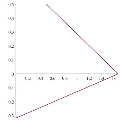
$X$ is obtained from the previous example, with $\alpha=-6/100$ and $\beta=4/100$ (region III). Consider the initial condition $P_{1}=(0.5,0.5).$ The trajectory of $X_{++}$ starting in $P_{1}$ is

(43)

x(t)=(277/1800)t+1/2,y(t)=-(59/900)t+1/2.

After $t=450/59$ , the trajectory reaches $\Sigma_{+0}$ at $P_{2}=(395/236,0)$ and as seen before, $\Sigma_{+0}$ is a sewing region. So we take the trajectory of $X_{+-}$ by $P_{2}$ when $t=450/59$

(44)

x(t)=-(623/1800)t+509/118,y(t)=-(59/900)t+1/2.

After $t=458100/36757$ the solution reaches $\Sigma_{0-}$ , which is a sliding manifold. Calculating the Filippov sliding vector field on $\Sigma_{0-}$ ,

X_{0-}^{sl}=\left[\begin{array}[]{c}0\\ \vskip 6.0pt plus 2.0pt minus 2.0pt\cr{\dfrac{1187}{900}}\end{array}\right]

and its trajectory by $P_{3}=(0,-395/1246)$ at $t=458100/36757$ , we get

(45)

x(t)=0,y(t)=(1187/900)t-1977/118.

Finally, after $t=\frac{1779300}{140066}$ the solution reaches and slides on $\Sigma_{00}$ as expected.

The straightline $x\left(t\right)=\frac{277t}{1800}-\frac{277}{3482}$ , $y\left(t\right)=\frac{1741t}{900}-1$ located in the third quadrant, Figure 13, delimits the attraction basin of $\Sigma_{00}$ (hatched region) and of $\Sigma_{-0}$ (no hatched region).

7. Acknowledgments

The authors are partially supported by CAPES and FAPESP. The authors are grateful for the suggestions and comments of Daniel Cantergiani Panazzolo and for the hospitality of LMIA-UNIVERSITÉ DE HAUTE-ALSACE.

References

[1] Buzzi, C., Carvalho, T., and da Silva, P.R. (2013). Closed poly-trajectories and Poincaré index of non-smooth vector fields on the plane, Journal of Dynamical and Control Systems 19, 633–655.
[2] Buzzi, C., Silva, P.R., and Teixeira, M.A. (2006). A Singular approach to discontinuous vector fields on the plane, J.Diff. Equations 231, 633–655.
[3] Diecci, L. (2015). Sliding motion on the intersection of two manifolds: spirally attractive case, Communications in Nonlinear Science and Numerical Simulation 26, 1–3, 65-74.
[4] Diecci, L., Difonzo, F. (2015). The Moments Sliding Vector Field on the Intersection of Two Manifolds, J. Dynam. Diff. Equation 29-1, 169–201.
[5] Diecci, L., Elia, C., Lopez, L. (2013). A Filippov sliding vector field on an attracting codimension 2 discontinuity surface, and a limited loss-of-attractivity analysis J. Diff. Equations 254, 1800–1832.
[6] Fenichel, N. (1979). Geometric singular perturbation theory for ordinary differential equations, J. Diff. Equations 31, 53–98.
[7] Filippov, A.F. (1988). Differential equations with discontinuous right–hand sides, Mathematics and its Applications (Soviet Series), Kluwer Academic Publishers, Dordrecht.
[8] Y. Kuznetsov (2004). Elements of Applied Bifurcation Theory, Springer-Verlag New York.
[9] Llibre, J., Silva, P.R. and Teixeira, M.A. (2007). Regularization of discontinuous vector fields via singular perturbation, J. Dynam. Diff. Equation 19-2, 309–331.
[10] Llibre, J., Silva, P.R. and Teixeira, M.A. (2008). Sliding vector fields via slow fast systems, Bulletin of the Belgian Mathematical Society Simon Stevin 15, 851–869.
[11] Llibre, J., Silva, P.R. and Teixeira, M.A. (2009). Study of Singularities in non smooth dynamical systems via Singular Perturbation, SIAM Journal on Applied Dynamical Systems 8, 508-526.
[12] Llibre, J., Silva, P.R. and Teixeira, M.A. (2015). Sliding vector fields for non-smooth dynamical systems having intersecting switching manifolds, Nonlinearity (Bristol. Print) 28, 493-507.
[13] Nev, O.A. and van den Berg, H.A. (2017). Microbial metabolism and growth under conditions of starvation modelled as the sliding mode of a differential inclusion, Dynamical Systems - An International Journal 33, 93–112.
[14] Panazzolo, D.C and Silva, P.R. (2017). Regularization of discontinuous foliations: Blowing up and sliding conditions via Fenichel theory, J.Diff. Equations 263, 8362–8390.
[15] Seidman, T.I. (2007) Some aspects of modeling with discontinuities. https://pdfs. semanticscholar.org/91ee/48cc825cb520fcdf79d4d3fb2fe7e6dab426.pdf
[16] Sotomayor, J. and Teixeira, M.A. (1996). Regularization of discontinuous vector fields, International Conference on Differential Equations, Lisboa, Equadiff 95, 207–223.
[17] Szmolyan, P. (1991). Transversal Heteroclinic and Homoclinic Orbits in Singular Perturbation Problems, J. Diff. Equations 92, 252–281.

Slow–fast systems and sliding on codimension 2 switching manifolds

Abstract.

Key words and phrases:

2010 Mathematics Subject Classification

1. Introduction

1.1. Set of discontinuity Σ⊆ℝn\Sigma\subseteq\mathbb{R}^{n} with codimension 2 points.

Definition 1.1.

2. Basic Tools

2.1. Singular Perturbation Tools

Theorem 2.1.

2.2. Sliding region depending on the regularization

Definition 2.1.

Definition 2.2.

Definition 2.3.

3. 22-cross and regularization curve (ε,k​ε)(\varepsilon,k\varepsilon)

Theorem 3.1.

Proof.

Example 1.

4. Sliding depending of the regularization curve

Proposition 4.1.

Proof.

Proposition 4.2.

Proof.

Theorem 4.1.

Proof.

Theorem 4.2.

Proof.

5. On the quadratic system (22)

Theorem 5.1.

Proof.

Proposition 5.1.

Proof.

Theorem 5.2.

Proof.

6. Examples

Example 2.

Example 3.

Example 4.

Example 5.

7. Acknowledgments

References

1.1. Set of discontinuity $\Sigma\subseteq\mathbb{R}^{n}$ with codimension 2 points.

3. $2$ -cross and regularization curve $(\varepsilon,k\varepsilon)$