SOTER: A Runtime Assurance Framework for Programming Safe Robotics Systems
Abstract
The recent drive towards achieving greater autonomy and intelligence in robotics has led to high levels of complexity. Autonomous robots increasingly depend on third-party off-the-shelf components and complex machine-learning techniques. This trend makes it challenging to provide strong design-time certification of correct operation.
To address these challenges, we present Soter, a robotics programming framework with two key components: (1) a programming language for implementing and testing high-level reactive robotics software, and (2) an integrated runtime assurance (RTA) system that helps enable the use of uncertified components, while still providing safety guarantees. Soter provides language primitives to declaratively construct a RTA module consisting of an advanced, high-performance controller (uncertified), a safe, lower-performance controller (certified), and the desired safety specification. The framework provides a formal guarantee that a well-formed RTA module always satisfies the safety specification, without completely sacrificing performance by using higher performance uncertified components whenever safe. Soter allows the complex robotics software stack to be constructed as a composition of RTA modules, where each uncertified component is protected using a RTA module.
To demonstrate the efficacy of our framework, we consider a real-world case-study of building a safe drone surveillance system. Our experiments both in simulation and on actual drones show that the Soter-enabled RTA ensures the safety of the system, including when untrusted third-party components have bugs or deviate from the desired behavior.
I Introduction
Robotic systems are increasingly playing diverse and safety-critical roles in society, including delivery systems, surveillance, and personal transportation. This drive towards autonomy is also leading to ever-increasing levels of software complexity, including integration of advanced data-driven, machine-learning components. This complexity comes on top of the existing challenge of designing safe event-driven, real-time, concurrent software required for robotics applications. However, advances in formal verification and systematic testing have yet to catch up with this increased complexity [1]. Moreover, the dependence of robotic systems on third-party off-the-shelf components and machine-learning techniques is predicted to increase. This has resulted in a widening gap between the complexity of systems being deployed and those that can be certified for safety and correctness.
One approach to bridging this gap is to leverage techniques for run-time assurance, where the results of design-time verification are used to build a system that monitors itself and its environment at run time; and, when needed, switches to a provably-safe operating mode, potentially at lower performance and sacrificing certain non-critical objectives. A prominent example of a Run-Time Assurance (RTA) framework is the Simplex Architecture [2], which has been used for building provably-correct safety-critical avionics [3, 4], robotics [5] and cyber-physical systems [6, 7, 8].
The typical RTA architecture based on Simplex [2] (see Figure 1) comprises three sub-components: (1) The advanced controller (AC) that controls the robot under nominal operating conditions, and is designed to achieve high-performance with respect to specialized metrics (e.g., fuel economy, time), but it is not provably safe, (2) The safe controller (SC) that can be pre-certified to keep the robot within a region of safe operation for the plant/robot, usually at the cost of lower performance, and (3) The decision module (DM) which is pre-certified (or automatically synthesized to be correct) to periodically monitor the state of the plant and the environment to determine when to switch from AC to SC so that the system is guaranteed to stay within the safe region. When AC is in control of the system, DM monitors (samples) the system state every period to check whether the system can violate the desired safety specification () in time . If so, then DM switches control to SC.

This Simplex-based RTA architecture is a very useful high-level framework, but there are several limitations of its existing instantiations. First, existing techniques either apply RTA [9, 10, 3] to a single untrusted component in the system or wrap the large monolithic system into a single instance of Simplex which makes the design and verification of the corresponding SC and DM difficult or infeasible. Second, most prior applications of RTA do not provide high-level programming language support for constructing provably-safe RTA systems in a modular fashion while designing for timing and communication behavior of such systems. In order to ease the construction of RTA systems, there is a need for a general programming framework for building provably-safe robotic software systems with run-time assurance that also considers implementation aspects such as timing and communication. Finally, existing techniques do not provide a principled and safe way for DM to switch back from SC to AC so as to keep performance penalties to a minimum while retaining strong safety guarantees.
In this paper, we seek to address these limitations by developing Soter, a programming framework for building safe robotics systems using runtime assurance. A Soter program is a collection of periodic processes, termed nodes, that interact with each other using a publish-subscribe model of communication (which is popular in robotics, e.g., in Robot Operating System, ROS [11]). An RTA module in Soter consists of an advanced controller node, a safe controller node and a safety specification; if the module is well-formed then the framework provides a guarantee that the system satisfies the safety specification. Soter allows programmers to declaratively construct an RTA module with specified timing behavior, combining provably-safe operation with the feature of using AC whenever safe so as to achieve good performance. Soter provides a provably-safe way for DM to switch back from SC to AC, thus extending the traditional RTA framework and providing higher performance. Our evaluation demonstrates that Soter is effective at achieving this blend of safety and performance.
Crucially, Soter supports compositional construction of the overall RTA system. The Soter language includes constructs for decomposing the design and verification of the overall RTA system into that for individual RTA modules while retaining guarantees of safety for the overall composite system. Soter includes a compiler that generates the DM node that implements the switching logic, and which also generates C code to be executed on common robotics software platforms such as ROS [11] and MavLink [12].
We evaluate the efficacy of the Soter framework by building a safe autonomous drone surveillance system. We show that Soter can be used to build a complex robotics software stack consisting of both third-party untrusted components and complex machine learning modules, and still provide system-wide correctness guarantees. The generated code for the robotics software has been tested both on an actual drone platform (the 3DR [13] drone) and in simulation (using the ROS/Gazebo [14] and OpenAI Gym [15]). Our results demonstrate that the RTA-protected software stack built using Soter can ensure the safety of the drone both when using unsafe third-party controllers and in the presence of bugs introduced using fault injection in the advanced controller.
In summary, we make the following novel contributions:
- 1.
A programming framework for a Simplex-based run-time assurance system that provides language primitives for the modular design of safe robotics systems (Sec. III);
- 2.
A theoretical formalism based on computing reachable sets that keeps the system provably safe while maintaining smooth switching behavior from advanced to a safe controller and vice-versa (Sec. III-C);
- 3.
A framework for the modular design of run-time assurance (Sec. IV), and
- 4.
Experimental results in simulation and on real drone platforms demonstrating how Soter can be used for guaranteeing correctness of a system even in the presence of untrusted or unverified components (Sec. V).
II Overview
We illustrate the Soter framework for programming safe robotics systems by using our case study of an autonomous drone surveillance system.
II-A Case Study: Drone Surveillance System
In this paper, we consider the problem of building a surveillance system where an autonomous drone must safely patrol a city. Figure 2 (left) presents a snapshot of the city workspace from the ROS/Gazebo simulator [14] and Figure 2 (right) presents the corresponding obstacle map.

For our case study, we consider a simplified setting where all the obstacles (houses, cars, etc.) are static, known a priori, and that there are no environment uncertainties like wind. Even for such a simplified setup the software stack (Figure 3) is complex: consisting of multiple components interacting with each other and uses uncertified components (red blocks).
Drone software stack. The application layer implements the surveillance protocol that ensures the application specific property, e.g., all surveillance points must be visited infinitely often. The generic components of the software stack consists of the motion planner and the motion primitives.
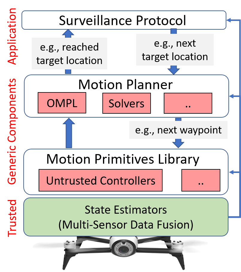
For surveillance, the application generates the next target location for the drone. The motion planner computes a sequence of waypoints from the current location to the target location – a motion plan. The waypoints in Figure 2 represent one such motion plan generated by the planner and the dotted lines represent the reference trajectory for the drone. Once the motion primitive library receives the next waypoint, it generates the required low-level controls necessary to closely follow the reference trajectory. The solid trajectory in Figure 2 represents the actual trajectory of the drone, which deviates from the reference trajectory because of the underlying dynamics. Programming such robotics software stack is challenging as it is composed of individual components, each implementing a complicated protocol, and continuously interacting with each other for accomplishing the mission safely.
In our drone surveillance case study, we would like the system to satisfy two safety invariants: (1) Obstacle Avoidance (): The drone must never collide with any obstacle. (2) Battery Safety (): The drone must never crash because of low battery. Instead, when the battery is low it must prioritize landing safely (e.g., in Figure 2 (right), low battery is detected at and the mission is aborted to land safely). can be further decomposed into two parts ; (a) Safe Motion Planner (): The motion planner must always generate a motion-plan such that the reference trajectory does not collide with any obstacle, (b) Safe Motion Primitives (): When tracking the reference trajectory between any two waypoints generated by the motion planner, the controls generated by the motion primitives must ensure that the drone closely follows the trajectory and avoids collisions.
In practice, when implementing the software stack, the programmer may use several uncertified components (red blocks in Figure 3). For example, implementing an on-the-fly motion planner may involve solving an optimization problem or using an efficient search technique that relies on a solver or a third-party library (e.g., OMPL [16]). Similarly, motion primitives are either designed using machine-learning techniques like Reinforcement Learning [17], or optimized for specific tasks without considering safety, or are off-the-shelf controllers provided by third parties [12]. Ultimately, in the presence of such uncertified or hard to verify components, it is difficult to provide formal guarantees of safety at design time. We assume the state-estimators (green blocks) in Figure 3 are trusted and accurately provide the system state within bounds.
Challenges and motivation: The robotics software (Figure 3) must react to events (inputs) from the physical world as well as other components in the software stack. These components must therefore be implemented as concurrent event-driven software which can be notoriously tricky to test and debug due to nondeterministic interactions with the environment and interleaving of the event handlers. In Soter, we provide a language framework for both implementing and systematic testing of such event-driven software. In practice, for complex systems, it can be extremely difficult to design a controller that is both safe and high-performance. The AC, in general, is any program or component designed for high-performance under nominal conditions using either third-party libraries or machine-learning techniques. We treat them as unsafe since they often exhibit unsafe behavior in off-nominal conditions and uncertain environments, and even when they do not, it is hard to be sure since their complexity makes verification or exhaustive testing prohibitively expensive. Furthermore, the trend in robotics is towards advanced, data-driven controllers, such as those based on neural networks (NN), that usually do not come with safety guarantees. Our approach of integrating RTA into a programming framework is motivated by the need to enable the use of such advanced controllers (e.g., designed using NN or optimized for performance) while retaining strong guarantees of safety.
II-B Programming Reactive Robotic Software
The Robot Operating System (ROS [11]) is an open-source meta-operating system considered as the de facto standard for robot software development. In most cases, a ROS programmer implements the system as a collection of periodic processes that communicates using the publish-subscribe model of communication. Soter provides a high-level domain specific language based on a similar publish-subscribe model of communication. A program in Soter is a collection of periodic nodes (processes) communicating with each other by publishing on and subscribing to message topics. A node periodically listens to data published on certain topics, performs computation, and publishes computed results on certain other topics. A topic is an abstraction of a communication channel.
Topics. Figure 4 declares the topic targetWaypoint that can be used to communicate messages of type coord (coordinates in 3D space). In Soter, a node communicates with other nodes in the system by publishing messages on a topic (e.g., targetWaypoint) and the target nodes can consume these messages by subscribing to it.
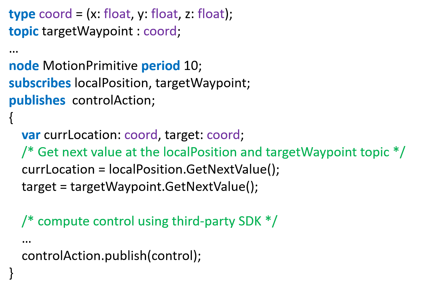
Nodes. Figure 4 also declares a node MotionPrimitive that subscribes to topics localPosition and targetWaypoint. Each node has a separate local buffer associated with each subscribed topic. The publish operation on a topic adds the message into the corresponding local buffer of all the nodes that have subscribed to that topic. The MotionPrimitive node runs periodically every 10 . It reads messages from the subscribed topics, performs local computations, and then publishes the control action on the output topic. For the exposition of this paper, we ignore the syntactic details of the node body, it can be any sequential program that performs the required read compute publish step.
II-C Guaranteeing Safety using Runtime Assurance
In practice, the motion primitives (e.g., MotionPrimitive node in Figure 4) might generate control actions to traverse the reference trajectory from current position to the target waypoint using a low-level controller provided by the third-party robot manufacturer (e.g., [12]). These low-level controllers generally use approximate models of the dynamics of the robot and are optimized for performance rather than safety, making them unsafe.

To demonstrate this, we experimented with the low-level controllers provided by the PX4 Autopilot [12] (Figure 5 (right)). The drone was tasked to repeatedly visit locations to in that order, i.e., the sequence of waypoints are passed to the MotionPrimitive node. The blue lines represent the actual trajectories of the drone. Given the complex dynamics of a drone and noisy sensors, ensuring that it precisely follows a fixed trajectory (ideally a straight line joining the waypoints) is extremely hard. The low-level controller (untrusted) optimizes for time and, hence, during high speed maneuvers the reduced control on the drone leads to overshoot and trajectories that collide with obstacles (represented by the red regions). We also conducted similar experiment with a different low-level controller designed using data-driven approach (Figure 5 (left)) where we tasked the drone to follow a eight loop. The trajectories in green represent the cases where the drone closely follows loop, the trajectories in red represent the cases the drone dangerously deviates from the reference trajectory. Note that in both cases, the controllers can be used during majority of their mission except for a few instances of unsafe maneuvers. This motivates the need for a RTA system that guarantees safety by switching to a safe controller in case of danger but also maximizes the use of the untrusted but performant controller under nominal conditions.
Runtime Assurance module. Figure 6 illustrates the behavior of a Soter based RTA-protected motion primitive module.

We want the drone to move from its current location to the target location , and the desired safety property is that the drone must always remain inside the region (outermost tube). Initially, the untrusted AC node (e.g., MotionPrimitive) is in control of the drone (red trajectory), and since it is not certified for correctness it may generate controls action that tries to push the drone outside the region. If AC is wrapped inside an RTA module (see Figure 1) then DM must detect this imminent danger and switch to SC (blue trajectory) with enough time for SC to gain control over the drone. SC must be certified to keep the drone inside and also move it to a state in where DM evaluates that it is safe enough to return control back to AC. The novel aspect of an RTA module formalized in this paper is that it also allows control to return back to AC to maximize performance.
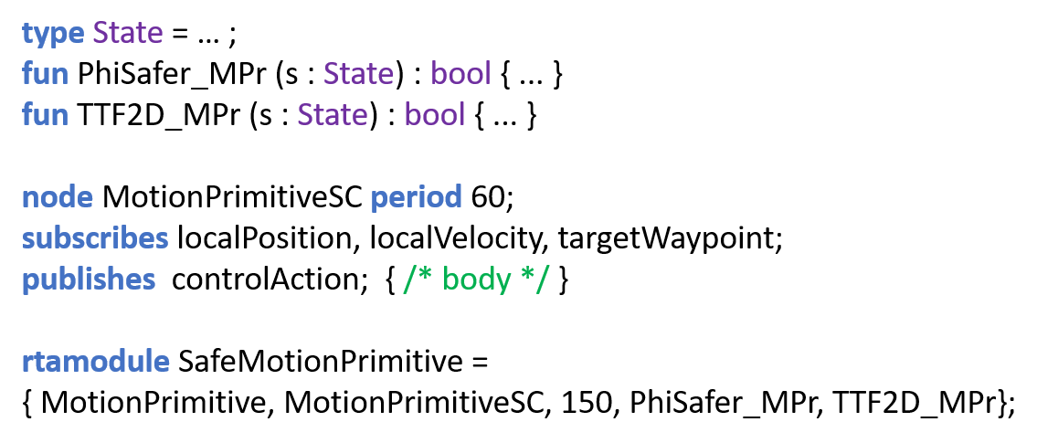
Figure 7 presents the declaration of an RTA module consisting of MotionPrimitive (from Figure 4) and MotionPrimitiveSC as AC and SC nodes. The compiler checks that the declared RTA module SafeMotionPrimitive is well-formed (Section III-C) and then generates the DM and the other glue code that together guarantees the property. Details about other components of the module declaration are provided in Section III-C.
Compositional RTA System. A large system is generally built by composing multiple components together. When the system-level specification is decomposed into a collection of simpler component-level specifications, one can scale provable guarantees to large, real-world systems.

Soter enables building a reliable version (Figure 8) of the software stack with runtime assurance of the safety invariant: . We decompose the stack into three components: (1) An RTA-protected motion planner that guarantees , (2) A battery-safety RTA module that guarantees , and (3) An RTA-protected motion primitive module that guarantees . Our theory of well-formed RTA modules (Theorem III.1) ensures that if the constructed modules are well-formed then they satisfy the desired safety invariant and their composition (Theorem IV.1) helps prove that the system-level specification is satisfied.
III Runtime Assurance Module
In this section, we formalize the Soter runtime assurance module and present the well-formedness conditions required for its correctness. We conclude by informally describing the behavior of a system protected by an RTA module.
III-A Programming Model
Recollect that a program in Soter is a collection of periodic nodes communicating with each other by publishing on and subscribing to message topics.
Topic. Formally, a topic is a tuple consisting of a unique name , where is the universe of all topic names, and a value , where is the universe of all possible values that can be communicated using topic . For simplicity of presentation: (1) we assume that all topics share the same set of possible values and (2) instead of modeling the local buffers associated with each subscribed topic of a node; we model the communication between nodes using the global value associated with each topic.
Let represent the set of names of all the nodes. We sometimes refer to a node by its unique name, for example, when and we say “node ”, we are referring to a node with name . Let represent the set of all possible values the local state of any node could have during its execution. A valuation of a set of topic names is a map from each topic name to the value stored at topic . Let represent the valuations of set .
Node. A node in Soter is a tuple where:
- 1.
is the unique name of the node.
- 2.
is the set of names of all topics subscribed to by the node (inputs).
- 3.
is the set of names of all topics on which the node publishes (output). The output topics are disjoint from the set of input topics ().
- 4.
is the transition relation of the node. If , then on the input (subscribed) topics valuation of , the local state of the node moves from to and publishes on the output topics to update its valuation to .
- 5.
is the time-table representing the times at which the node takes a step.
Intuitively, a node is a periodic input-output state-transition system: at every time instant in its calendar, the node reads the values in its input topics, updates its local state, and publishes values on its output topics. Note that we are using the timeout-based discrete event simulation [18] to model the periodic real-time process as a standard transition system (more details in Section IV). Each node specifies, using a time-table, the fixed times at which it should be scheduled. For a periodic node with period , the calendar will have entries such that for all . We refer to the components of a node with name as and respectively. We use to refer to the period of node .
III-B Runtime Assurance Module
Let represent the state space of the system, i.e., the set of all possible configurations of the system (formally defined in Section IV). We assume that the desired safety property is given in the form of a subset (safe states). The goal is to ensure using an RTA module that the system always stays inside the safe set .
RTA Module. An RTA module is represented as a tuple where:
- 1.
is the advanced controller (AC) node,
- 2.
is the safe controller (SC) node,
- 3.
is the decision module (DM) node,
- 4.
represents the period of DM (),
- 5.
is the desired safety property.
- 6.
is a stronger safety property.

Given an RTA module , Figure 9 presents the switching logic that sets the mode of the RTA module given the current state of the system. The DM node evaluates this switching logic once every time unit. When it runs, it first reads the current state and sets based on it. Note that the set determines when it is safe to switch from to . represents the set of all states reachable in time starting from the state , using any non-deterministic controller. We formally define in Section IV, informally, checks that the system will remain inside in the next time. This look ahead is used to determine when it is necessary to switch to using , in order to ensure that the () will be executed at least once before the system leaves . The Soter compiler automatically generates a unique DM node () for each primitive RTA module declaration.
For an RTA module , DM is the node where:
- 1.
The local state is a binary variable mode : .
- 2.
Topics subscribed by DM include the topics subscribed by either of the nodes; i.e., and .
- 3.
DM does not publish on any topic. But it updates a global data structure that controls the outputs of AC and SC nodes (more details in Section IV).
- 4.
If , then the local state moves from to based on the logic in Figure 9.
- 5.
where represents the time-table of the node.
III-C Correctness of an RTA Module
Given a safe set , our goal is to prove that the RTA-protected system always stays inside this safe set. We need the RTA module to satisfy some additional conditions in order to prove its safety.
Well-formed RTA Module. An RTA module is said to be well-formed if its components satisfy the following properties:
(P1a) The maximum period of and is , i.e., , , and .
(P1b) The output topics of the and nodes must be same, i.e., .
The safe controller, , must satisfy the following properties:
(P2a) (Safety) . This property ensures that if the system is in , then it will remain in that region as long as we use .
(P2b) (Liveness) For every state , there exists a time such that for all , we have . In words, from every state in , after some finite time the system is guaranteed to stay in for at least time.
(P3) . This condition says that irrespective of the controller, if we start from a state in , we will continue to remain in for time units. Note that this condition is stronger than the condition .
Theorem III.1 (Runtime Assurance)
For a well-formed RTA module , let denote the predicate . If the initial state satisfies the invariant , then every state reachable from will also satisfy the invariant .
Proof.
Let be the initial mode and initial state of the system.
We are given that the invariant holds at this state.
Since the initial mode is SC, then, by assumption, .
We need to prove that all states reachable from also satisfy the invariant.
If there is no mode change, then invariant is satisfied by Property (P2a).
Hence, assume there are mode switches.
We prove that in every time interval between two consecutive executions of the DM, the invariant holds.
So, consider time when the DM executes.
(Case1) The mode at time is SC and there is no mode switch at this time.
Property (P2a) implies that all future states will satisfy the invariant.
(Case2)
The mode at time is SC and there is a mode switch to the AC at this time.
Then, the current state at time satisfies the condition .
By Property (P3), we know that , and hence,
it follows that
, and hence the invariant holds at time .
In fact, irrespective of what actions AC applies to the plant, Property (P3) guarantees that
the invariant will hold for the interval .
Now, it follows from Property (P1) that the DM will execute again at or before
the time instant , and hence the invariant holds until the next execution of DM.
(Case3)
The current mode at time is AC and there is a mode switch to SC at this time.
Then, the current state at time satisfies the condition
.
Since the mode at time was still AC, and by inductive hypothesis we know that the
invariant held at that time; therefore,
we know that . Therefore,
for the period , we know that the reached state will be in
and the invariant holds.
Moreover, SC will get a chance to execute in this interval at least once, and
hence, from that time point onwards, Property (P2a) will guarantee that the invariant holds.
(Case4)
The current mode at time is AC and there is a no mode switch.
Since there is no mode switch at , it implies that
and hence for the next time units,
we are guaranteed that
holds.
The invariant established in Theorem III.1 ensures that if the assumptions of the theorem are satisfied, then all reachable states are always contained in .
Remark III.1 (Guarantee switching and avoid oscillation)
The liveness property (P2b) guarantees that the system will definitely switch from to (to maximize performance). Property (P3) ensures that the system will stay in the AC mode for some time and not switch back immediately to the SC mode. Note that property (P2b) is not needed for Theorem III.1.
Remark III.2 (AC is a black-box)
Our well-formedness check does not involve proving anything about . (P1a) and (P1b) require that samples at most as fast as and generates the same outputs as , this is for smooth transitioning between and . We only need to reason about , and we need to reason about all possible controller actions (when reasoning with ). The latter is worst-case analysis, and includes ’s behavior. One could restrict behaviors to if we wanted to be more precise, but then would not be a black-box anymore.
Our formalism makes no assumptions about the code (behavior) of the AC node, except that we do need to know the set of all possible output actions (required for doing worst-case reachability analysis). Theorem 3.1 ensures safety as long as all output actions generated by the code AC (like in Figure 4) belong to the assumed set of all possible actions.
Definition III.1 (Regions)
Let . For example, represents the region or set of states in from which all reachable states in time are still in .
Regions of operation of a well-formed RTA module. We informally describe the behavior of an RTA protected module by organizing the state space of the system into different regions of operation (Figure 10). R1 represents the unsafe region of operation for the system. Regions R2-R5 represent the safe region and R3-R5 are the recoverable regions of the state space. The region R3R4 represents the switching control region (from AC to SC) as the time to escape for the states in this region is less than .

As the DM is guaranteed to sample the state of the system at least once in time (property (P1a)), the DM is guaranteed to switch control from AC to SC if the system remains in the switching control region for at least time, which is the case before system can leave region R3. Consider the case where T1 represents a trajectory of the system under the influence of AC, when the system is in the switching control region the DM detects the imminent danger and switches control to SC. (P1a) ensures that takes control before the system escapes in the next time. Property (P2a) ensures that the resultant trajectory T2 of the system remains inside the safe region and Property (P2b) ensures that the system eventually enters region R5 where the control can be returned to AC for maximizing the performance of the system. Property (P3) ensures that the switch to AC is safe and the system will remain in AC mode for at least time.
Remark III.3 (Choosing and )
The value of is critical for ensuring safe switching from AC to SC. It also determines how conservatively the system behaves: for example, large value of implies a large distance between boundaries of region R4 and R5 during which SC (conservative) is in control. Small values of and a larger R5 region () can help maximize the use of AC but might increase the chances of switching between AC and SC as the region between the boundaries of R4 and R5 is too small. Currently, we let the programmer choose these values and leave the problem of automatically finding the optimal values as future work.
From theory to practice: We are assuming here that the checks in Property (P2) and Property (P3) can be performed. The exact process for doing so is outside the scope of this paper. The popular approach in control theory is to use reachability analysis when designing an that always keeps the system within a set of safe states. We used existing tools like FastTrack [19] and the Level-Set Toolbox [20].
First, consider the problem of synthesizing the safe controller for a given safe set . can be synthesized using pre-existing safe control synthesis techniques. For example, for the motion primitives, we can use a framework like FaSTrack [19] for synthesis of low-level . Next, we note that the DM needs to reason about the reachable set of states for a system when either the controller is fixed to or is nondeterministic. Again, there are several tools and techniques for performing reachability computations [20]. One particular concept that Soter requires here is the notion of time to failure less than 2 (). The function , given a state and a predicate returns true if starting from , the minimum time after which may not hold is less than or equal to . The check in Figure 9 can be equivalently described using the function as . Let us revisit the boolean functions PhiSafer_MPr and TTF2D_MPr from Figure 7, these functions correspond to the checks and respectively.
IV Operational Semantics of an RTA Module
In Soter, a complex system is designed as a composition of RTA modules. An RTA system is a set of composable RTA modules. A set of modules are composable if:
- 1.
The nodes in all modules are disjoint, if , , and represent the AC, SC and DM nodes of a module then, for all s.t. , .
- 2.
The outputs of all modules are disjoint, for all s.t. , .
Note that only constraint for composition is that the outputs (no constraints on inputs) must be disjoint as described by traditional compositional frameworks like I/O Automata and Reactive Modules [21, 22].
Composition. If RTA modules and are composable then their composition is an RTA system consisting of the two modules . Also, composition of two RTA systems and is an RTA system , if all modules in are composable.
Theorem IV.1 (Compositional RTA System)
Let be an RTA system. If for all , is a well-formed RTA module satisfying the safety invariant then, satisfies the invariant .
Proof. Note that this theorem simply follows from the fact that composition just restricts the environment. Since we are guaranteed output disjointness during composition, composition of two modules is guaranteed to be language intersection. The proof for such composition theorem is described in details in [21, 22].
Theorem IV.1 plays an important role in building the reliable software stack in Figure 2c. Each RTA module individually satisfies the respective safety invariant and their composition helps establish the system-level specification.
We use to refer to the domain of map and to refer to the codomain of . Given an RTA system , its attributes (used for defining the operational semantics) can be inferred as follows:
- 1.
is a map that binds a DM node to the particular AC node it controls, i.e., if then .
- 2.
is a map that binds a DM node to the particular SC node it controls, i.e., if then .
- 3.
represents the set of all nodes in the RTA system, .
- 4.
represents the set of outputs of the RTA system, .
- 5.
represents the set of inputs of the RTA system (inputs from the environment), .
- 6.
represents the calendar or time-table of the RTA system, .
We refer to the attributes of a RTA system as , , , , , and respectively.
We next present the semantics of an RTA system. Note that the semantics of an RTA module is the semantics of an RTA system where the system is a singleton set. We use the timeout-based discrete event simulation model [18] for modeling the semantics of an RTA system. The calendar stores the future times at which nodes in the RTA system must step. Using a variable to store the current time and to store the enabled nodes, we can model the real-time system as a discrete transition system.
Configuration. A configuration of an RTA system is a tuple where:
- 1.
represents a map from a node to the local state of that node.
- 2.
represents a map from a node to a boolean value indicating whether the output of the node is enabled or disabled. This is used for deciding whether AC or SC should be in control. The domain of is .
- 3.
represents the current time.
- 4.
represents the set of nodes that are remaining to be fired at time .
- 5.
is a map from a topic name to the value stored at that topic, it represents the globally visible topics. If then represents a map from each to .
The initial configuration of any RTA system is represented as where: maps each node in its domain to default local state value if the node is AC or SC, otherwise, for the DM node, maps each SC node to true and AC node to false (this is to ensure that each RTA module starts in SC mode), , , and maps each topic name to its default value .
We represent the operational semantics of a RTA system as a transition relation over its configurations (Figure 11).
There are two types of transitions: (1) discrete transitions that are instantaneous and hence does not change the current time, and (2) time-progress transitions that advance time when no discrete transition is enabled. DM-Step and AC-or-SC-Step are the discrete transitions of the system. Environment-Input transitions are triggered by the environment and can happen at any time. It updates any of the input topics of the module to . Discrete-Time-Progress-Step represents the time-progress transitions that can be executed when no discrete transitions are enabled (dt1). It updates to the next time at which a discrete transition must be executed (dt2). is updated to the set of nodes that are enabled and must be executed (dt3) at the current time. DM-Step represents the transition of any of the DM nodes in the module. The important operation performed by this transition is to enable or disable the outputs of the AC and SC node (dm2) based on its current mode (dm1). Finally, AC-or-SC-Step represents the step of any AC or SC node in the module. Note that the node updates the output topics only if its output is enabled (based on (n1)).
Reachability. Note that the state space of an RTA system is the set of all possible configurations. The set of all possible reachable states of an RTA system is a set of configurations that are reachable from the initial configuration using the transition system described in Figure 11. Since the environment transitions are nondeterministic, potentially many states are reachable even if the RTA modules are all deterministic.
Let represent the set of all states of the RTA system reachable in time starting from the state , using only the controller SC node of the RTA module . In other words, instead of switching control between SC and AC of the RTA module , the DM always keeps SC node in control. represents the set of all states of the RTA system reachable in time starting from the state , using only a completely nondeterministic module instead of . In other words, instead of module , a module that generates nondeterministic values on the output topics of is used. The notation is naturally extended to a set of states: is the set of all states reachable in time when starting from a state using . Note that, .
We note that the definition of DM for an RTA module is sensitive to the choice of the environment for . Consequently, every attribute of (such as well-formedness) depends on the context in which resides. We implicitly assume that all definitions of are based on a completely nondeterministic context. All results hold for this interpretation, but they also hold for any more constrained environment.
V Evaluation
We empirically evaluate the Soter framework by building an RTA-protected software stack (Figure 8) that satisfies the safety invariant: . The goal of our evaluation is twofold: (Goal1) Demonstrate how the Soter programming framework can be used for building the software stack compositionally, where each component is guaranteed to satisfy the component-level safety specification. Further, we show how the programmable switching feature of an RTA module can help maximize its performance. (Goal2) Empirically validate using rigorous simulations that an RTA-protected software stack can ensure the safety of the drone in the presence of third-party (or machine learning) components, where otherwise, the drone could have crashed.
The videos and other details corresponding to our experiments on real drones are available on https://drona-org.github.io/Drona/.
Soter tool chain. The Soter tool-chain consists of three components: the compiler, a C runtime and a backend systematic testing engine. The compiler first checks that all the constructed RTA modules in the program are well-formed. The compiler then converts the source-level syntax of a Soter program into C code. This code contains statically-defined C array-of-structs and functions for the topics, nodes, and functions declarations. The that controls the output of each node is implemented as a shared-global data-structure updated by all the DM in the program. The Soter C runtime executes the program according to the program’s operational semantics by using the C representation of the nodes. The periodic behavior of each node was implemented using OS timers for our experiments, deploying the generated code on real-time operating system is future work.
The compiler also generates C code that can be systematically explored by the backend testing engine. This part of the Soter framework is built on top of our previous work [23] on the P [24, 25] language and the Drona [26] robotics framework. The systematic testing engine enumerates, in a model-checking style, all possible executions of the program by controlling the interleaving of nodes using an external scheduler. Since a Soter program is a multi-rate periodic system, we use a bounded-asynchronous scheduler [27] to explore only those schedules that satisfy the bounded-asynchrony semantics. When performing systematic testing of the robotics software stack the third-party (untrusted) components that are not implemented in Soter are replaced by their abstractions implemented in Soter. The systematic testing backend details is not provided as the focus of our paper is to demonstrate the importance of runtime assurance after design-time analysis.
Experimental Setup For our experiments on the real drone hardware, we use a 3DR Iris [13] drone that comes with the open-source Pixhawk PX4 [12] autopilot. The simulation results were done in the Gazebo [14] simulator environment that has high fidelity models of Iris drone. For our simulations, we execute the PX4 firmware in the loop.


V-A RTA-Protected Safe Motion Primitives
A drone navigates in the 3D space by tracking trajectories between waypoints computed by the motion planner. Given the next waypoint, an appropriate motion primitive is used to track the reference trajectory. Informally, a motion primitive consists of a pre-computed control law (sequence of control actions) that regulates the state of the drone as a function of time. For our experiments in Figure 5, we used the motion primitives provided by the PX4 autopilot [12] as our advanced controller and found that it can lead to failures or collision.
To achieve RTA-protected motion primitive, there are three essential steps: (1) Design of the safe controller ; (2) Designing the function that controls switching from the AC to SC for the motion primitive; (3) Programming the switching from SC to AC and choosing an appropriate and so that the system is not too conservative.
When designing the , it must satisfy the Property (P2), where is the region not occupied by any obstacle. Techniques from control theory, like reachability [28] can be used for designing . We use the FaSTrack [19] tool for generating a correct-by-construction controller for the drone such that it satisfies all the properties required for a .
To design the switching condition from AC to SC, we need to compute the function that checks (Figure 9) where is the current state. Consider the 2D representation of the workspace (Figure 2) in Figure 12b. The obstacles (shown in grey) represent the region and any region outside is . Note that, can guarantee safety for all locations in (P2). We can use the level set toolbox [28] to compute the backward reachable set from in (shown in yellow), i.e., the set of states from where the drone can leave (collide with obstacle) in . In order to maximize the performance of the system, the RTA module must switch from SC to AC after the system has recovered. In our experiments, we choose (shown in green). is designed such that given , Property (P2b) holds. DM transfers control to AC when it detects that the drone is in , which is the backward reachable set from in time.
Choosing the period is an important design decision. Choosing a large can lead to overly-conservative and . In other words, a large pushes the switching boundaries further away from the obstacle. In which case, a large part of the workspace is covered by red or yellow region where SC (conservative controller) is in control.
We implemented the safe motion primitive as a RTA module using the components described above. Figure 12a presents one of the interesting trajectories where the SC takes control multiple times and ensures the overall correctness of the mission. The green tube inside the yellow tube represents the region. The red dots represent the points where the DM switches control to SC and the green dots represent the points where the DM returns control back to the AC for optimizing performance. The average time taken by the drone to go from to is 10 secs when only the unsafe is in control (can lead to collisions), it is 14 secs when using the RTA protected safe motion primitive, and 24 secs when only using the safe controller. Hence, using RTA provides a “safe” middle ground without sacrificing performance too much.
Figure 12b presents the 2D representation of our workspace in Gazebo (Figure 2a). The dotted lines represent one of the reference trajectories of the drone during the surveillance mission. The trajectory in solid shows the trajectory of the drone when using the RTA-protected software stack consisting of the safe motion primitive. At N1 and N2, the takes control and pushes the drone back into (green); and returns control back to . We observe that the is in control for the most part of the surveillance mission even in cases when the drone deviates from the reference trajectory (N3) but is still safe.
V-B RTA-Protected Battery Safety
We want our software stack to provide the battery-safety guarantee, that prioritizes safely landing the drone when the battery charge falls below a threshold level.
We first augment the state of the drone with the current battery charge, . is a node that receives the current motion plan from the planner and simply forwards it to the motion primitives module. is a certified planner that safely lands the drone from its current position. The set of all safe states for the battery safety is given by, , i.e., the drone is safe as long as the battery does not run out of charge. We define , i.e., the battery charge is greater than . Since the battery discharges at a slower rate compared to changes in the position of the drone, we define a larger for the battery RTA compared to the motion primitive RTA.
To design the , we first define two terms: (1) Maximum battery charge required to land ; and (2) Maximum battery discharge in , . In general depends on the current position of the drone. However, we approximate as the battery required to land from the maximum height attained by the drone safely. Although conservative, it is easy to compute and can be done offline. To find , we first define a function , which given the low-level control to the drone and a time period, returns the amount of battery the drone discharges by applying that control for the given time period. Then, is the maximum discharge that occurs in time across all possible controls, . We can now define . It guarantees that DM switches control to SC if the current battery level may not be sufficient to safely land if AC were to apply the worst possible control. DM returns control to once the drone is sufficiently charged. This is defined by , which is chosen to assert that the battery has at least charge before DM can hand control back to AC. The resultant RTA module is well-formed and satisfies the battery safety property . We implemented the battery safety RTA module with the components defined above. Figure 12c shows a trajectory, where the battery falls below the safety threshold causing DM to transfer control to which lands the drone.
V-C RTA for Safe Motion Planner
We use OMPL [16], a third-party motion-planning library that implements many state-of-the-art sampling-based motion planning algorithms. We implemented the motion-planner for our surveillance application using the RRT* [29] algorithm from OMPL. We injected bugs into the implementation of RRT* such that in some cases the generated motion plan can collide with obstacles. We wrapped the motion-planner inside an RTA module to ensure that the waypoints generated by motion plan do not collide with an obstacle (violating ).
To summarize, we used the theory of well-formed RTA module to construct three RTA modules: motion primitives, battery safety, and motion planner. We leverage Theorem III.1 to ensure that the modules individually satisfy the safety invariants , , and respectively. The RTA-protected software stack (Figure 2c) is a composition of the three modules and using Theorem IV.1 we can guarantee that the system satisfies the desired safety invariant .
V-D Rigorous Simulation
To demonstrate that Soter helps build robust robotics systems we conducted rigorous stress testing of the RTA-protected drone software stack. We conducted software in the loop simulations for 104 hours, where an autonomous drone is tasked to visit randomly generated surveillance points in the Gazebo workspace repeatedly (Figure 2). In total, the drone flew for approximately 1505K meters in the 104 hours of simulation. We found that there were 109 disengagements, these are cases where one of the SC nodes took control from AC and avoided a potential failure. There were 34 crashes during the experiments, and we found that in all these cases the problem was that the DM node did switch control, but the SC node was not scheduled in time for the system to recover. We believe that these crashes can also be avoided by running the software stack on a real-time operating system. We also found that as the RTA module is designed to return the control to AC after recovering the system, during our simulations, AC nodes were in control for of the time. Thus, safety is ensured without sacrificing the overall performance.
VI Related Work
We next situate Soter with related techniques for building robotics systems with high-assurance of correctness [30].
Reactive synthesis. There is increasing interest towards synthesizing reactive robotics controllers from temporal logic [31, 32, 33, 34]. Tools like TuLip [35], BIP [36, 37], and LTLMoP [38] construct a finite transition system that serves as an abstract model of the physical system and synthesizes a strategy, represented by a finite state automaton, satisfying the given high-level temporal specification. Though the generated strategy is guaranteed to be safe in the abstract model of the environment, this approach has limitations: (1) there is gap between the abstract models of the system and its actual behavior in the physical world; (2) there is gap between the generated strategy state-machine and its actual software implementation that interacts with the low-level controllers; and finally (3) the synthesis approach scale poorly both with the complexity of the mission and the size of the workspace. Recent tools such as SMC [34] generate both high-level and low-level plans, but still need additional work to translate these plans into reliable software on top of robotics platforms.
Reachability analysis and Simulation-based falsification. Reachability analysis tools [20, 39, 40] have been used to verify robotics systems modeled as hybrid systems. Differently from our work, reachability methods require an explicit representation of the robot dynamics and often suffer from scalability issues when the system has a large number of discrete states. Also, the analysis is performed using the models of the system, and hence, there is a gap between the models being verified and their implementation. Simulation-based tools for the falsification of CPS models (e.g., [41]) are more scalable than reachability methods, but generally, they do not provide any formal guarantees. In this approach, the entire robotics software stack is tested by simulating it in a loop with a high-fidelity model of the robot and hence, this approach does not suffer from the gap between model and implementation described in the previous approaches. However, a challenge to achieving scalable coverage comes from the considerable time it can take for simulations.
Runtime Verification and Assurance. Runtime verification has been applied to robotics [42, 43, 44, 45, 46, 47, 48] where online monitors are used to check the correctness (safety) of the robot at runtime. Schierman et al. [3] investigated how the RTA framework can be used at different levels of the software stack of an unmanned aircraft system. In a more recent work [10], Schierman et. al. proposed a component-based simplex architecture (CBSA) that combines assume-guarantee contracts with RTA for assuring the runtime safety of component-based cyber-physical systems. In [6], the authors apply simplex approach for sandboxing cyber-physical systems and present automatic reachability based approaches for inferring switching conditions. The idea of using an advanced controller (AC) under nominal conditions; while at the boundaries, using optimal safe control (SC) to maintain safety has also been used in [49] for operating quadrotors in the real world. In [50] the authors use a switching architecture ([51]) to switch between a nominal safety model and learned performance model to synthesize policies for a quadrotor to follow a trajectory. Recently, ModelPlex [52] combines offline verification of CPS models with runtime validation of system executions for compliance with the model to build correct by construction runtime monitors which provides correctness guarantees for CPS executions at runtime. Note that most prior applications of RTA do not provide high-level programming language support for constructing provably-safe RTA systems in a compositional fashion while designing for timing and communication behavior of such systems. They are all instances of using RTA as a design methodology for building reliable systems in the presence of untrusted components.
Soter approach. In order to ease the construction of RTA systems, there is a need for a general programming framework that supports run-time assurance principles and also considers implementation aspects such as timing and communication. Our approach is to provide a high-level language to (1) enable programmers to implement and specify the complex reactive system, (2) leverage advances in scalable systematic-testing techniques for validation of the actual implementation of the software, and (3) provide language support for runtime assurance to ensure safety in the real physical world. We formalize a generic runtime assurance architecture and implement it in programming framework for mobile robotic systems. We demonstrate the efficacy of Soter framework by building a real-world drone software stack and conducted rigorous experiments to demonstrate safety of autonomous robots in the presence of untrusted components. Also, note that most of the work done in the context of runtime assurance techniques provide solutions where the switching logic in DM is only configured to switch the control from AC to SC. In our architecture, the programmer can also specify the condition under which to transfer control back to AC, and maximize the use of AC during a mission.
VII Conclusion and Future Directions
In this paper, we have presented Soter, a new run-time assurance (RTA) framework for programming safe robotics systems. In contrast with other RTA frameworks, Soter provides (1) a programming language for modular implementation of safe robotics systems by combining each advanced controller with a safe counterpart; (2) theoretical results showing how to safely switch between advanced and safe controllers, and (3) experimental results demonstrating Soter on drone platforms in both simulation and in hardware.
Combining multiple RTA modules that have coordinated (DM) switching is non-trivial. A system may have multiple components with different guarantees. Our philosophy in this paper is that each component must then use an RTA instance to assure its guarantees, as this decomposition can help in building complex systems. Let’s consider a system consisting of two RTA modules M1 and M2, when M1 switches modes (AC to SC), it may require M2 to switch as well so that it can use the guarantee that M2’s new controller (SC) provides. This kind of coordinated switching complicates the overall architecture but is an interesting future work. We also plan to extend the experimental evaluation for a broader class of robotics platforms (e.g., multi-robot systems), safety specifications (e.g., probabilistic properties), and unknown environments (e.g., dynamic obstacles). Altogether, such extensions will enable us to make further progress towards the goal of verified intelligent autonomous systems [1].
Acknowledgments
We sincerely thank the anonymous reviewers and our shepherd Mohamed Kaaniche for their thoughtful comments. We also thank Daniel Fremont for his valuable feedback and suggested improvements on the previous drafts of the paper. This work was supported in part by the TerraSwarm Research Center, one of six centers supported by the STARnet phase of the Focus Center Research Program (FCRP) a Semiconductor Research Corporation program sponsored by MARCO and DARPA, by the DARPA BRASS and Assured Autonomy programs, by NSF grants 1545126 (VeHICaL), 1739816, and 1837132, by Berkeley Deep Drive, and by Toyota under the iCyPhy center.
References
- [1] S. A. Seshia, D. Sadigh, and S. S. Sastry, “Towards Verified Artificial Intelligence,” ArXiv e-prints, July 2016.
- [2] L. Sha, “Using simplicity to control complexity,” IEEE Software, vol. 18, no. 4, pp. 20–28, July 2001.
- [3] J. D. Schierman, M. D. DeVore, N. D. Richards, N. Gandhi, J. K. Cooper, K. R. Horneman, S. Stoller, and S. Smolka, “Runtime assurance framework development for highly adaptive flight control systems,” Barron Associates, Inc. Charlottesville, Tech. Rep., 2015.
- [4] D. Seto, E. Ferriera, and T. Marz, “Case study: Development of a baseline controller for automatic landing of an f-16 aircraft using linear matrix inequalities (lmis),” Software Engineering Institute, Carnegie Mellon University, Pittsburgh, PA, Tech. Rep. CMU/SEI-99-TR-020, 2000. [Online]. Available: http://resources.sei.cmu.edu/library/asset-view.cfm?AssetID=13489
- [5] D. Phan, J. Yang, R. Grosu, S. A. Smolka, and S. D. Stoller, “Collision avoidance for mobile robots with limited sensing and limited information about moving obstacles,” Formal Methods in System Design, vol. 51, no. 1, pp. 62–86, Aug 2017. [Online]. Available: https://doi.org/10.1007/s10703-016-0265-4
- [6] S. Bak, K. Manamcheri, S. Mitra, and M. Caccamo, “Sandboxing controllers for cyber-physical systems,” in 2011 IEEE/ACM Second International Conference on Cyber-Physical Systems, April 2011, pp. 3–12.
- [7] M. Clark, X. Koutsoukos, R. Kumar, I. Lee, G. Pappas, L. Pike, J. Porter, and O. Sokolsky, “Study on run time assurance for complex cyber physical systems,” Air Force Research Lab, Tech. Rep. ADA585474, April 2013, available at https://leepike.github.io/pubs/RTA-CPS.pdf.
- [8] S. Bak, D. K. Chivukula, O. Adekunle, M. Sun, M. Caccamo, and L. Sha, “The system-level simplex architecture for improved real-time embedded system safety,” in 2009 15th IEEE Real-Time and Embedded Technology and Applications Symposium, April 2009, pp. 99–107.
- [9] B. Bohrer, Y. K. Tan, S. Mitsch, M. O. Myreen, and A. Platzer, “Veriphy: Verified controller executables from verified cyber-physical system models,” SIGPLAN Not., vol. 53, no. 4, pp. 617–630, Jun. 2018. [Online]. Available: http://doi.acm.org/10.1145/3296979.3192406
- [10] D. Phan, J. Yang, M. Clark, R. Grosu, J. D. Schierman, S. A. Smolka, and S. D. Stoller, “A component-based simplex architecture for high-assurance cyber-physical systems,” arXiv preprint arXiv:1704.04759, 2017.
- [11] M. Quigley, K. Conley, B. P. Gerkey, J. Faust, T. Foote, J. Leibs, R. Wheeler, and A. Y. Ng, “Ros: an open-source robot operating system,” in ICRA Workshop on Open Source Software, 2009.
- [12] “PX4 Autopilot,” https://pixhawk.org/, 2017.
- [13] “3D Robotics,” https://3dr.com/, 2017.
- [14] N. Koenig and A. Howard, “Design and use paradigms for gazebo, an open-source multi-robot simulator,” in In IEEE/RSJ International Conference on Intelligent Robots and Systems, 2004, pp. 2149–2154.
- [15] G. Brockman, V. Cheung, L. Pettersson, J. Schneider, J. Schulman, J. Tang, and W. Zaremba, “Openai gym,” 2016.
- [16] I. A. Şucan, M. Moll, and L. E. Kavraki, “The Open Motion Planning Library,” IEEE Robotics & Automation Magazine, 2012.
- [17] L. P. Kaelbling, M. L. Littman, and A. W. Moore, “Reinforcement learning: A survey,” Journal of artificial intelligence research, vol. 4, pp. 237–285, 1996.
- [18] B. Dutertre and M. Sorea, “Modeling and verification of a fault-tolerant real-time startup protocol using calendar automata,” in Formal Techniques, Modelling and Analysis of Timed and Fault-Tolerant Systems, Y. Lakhnech and S. Yovine, Eds. Berlin, Heidelberg: Springer Berlin Heidelberg, 2004, pp. 199–214.
- [19] S. L. Herbert, M. Chen, S. Han, S. Bansal, J. F. Fisac, and C. J. Tomlin, “FaSTrack: A modular framework for fast and guaranteed safe motion planning,” in 2017 IEEE 56th Annual Conference on Decision and Control (CDC), Dec 2017, pp. 1517–1522.
- [20] G. Frehse, C. Le Guernic, A. Donzé, S. Cotton, R. Ray, O. Lebeltel, R. Ripado, A. Girard, T. Dang, and O. Maler, “SpaceEx: Scalable verification of hybrid systems,” in Computer Aided Verification, G. Gopalakrishnan and S. Qadeer, Eds. Berlin, Heidelberg: Springer Berlin Heidelberg, 2011, pp. 379–395.
- [21] R. Alur and T. A. Henzinger, “Reactive modules,” Formal methods in system design, vol. 15, no. 1, pp. 7–48, 1999.
- [22] N. A. Lynch and M. R. Tuttle, “An introduction to input/output automata,” 1988.
- [23] A. Desai, S. Qadeer, and S. A. Seshia, “Programming safe robotics systems: Challenges and advances,” in Leveraging Applications of Formal Methods, Verification and Validation. Verification - 8th International Symposium, ISoLA 2018, Limassol, Cyprus, November 5-9, 2018, Proceedings, Part II, 2018, pp. 103–119. [Online]. Available: https://doi.org/10.1007/978-3-030-03421-4\_8
- [24] A. Desai, V. Gupta, E. Jackson, S. Qadeer, S. Rajamani, and D. Zufferey, “P: Safe asynchronous event-driven programming,” in Programming Language Design and Implementation (PLDI), 2013.
- [25] A. Desai, A. Phanishayee, S. Qadeer, and S. A. Seshia, “Compositional programming and testing of dynamic distributed systems,” Proceedings of the ACM on Programming Languages (PACMPL) (OOPSLA), 2018.
- [26] A. Desai, I. Saha, J. Yang, S. Qadeer, and S. A. Seshia, “DRONA: A framework for safe distributed mobile robotics,” in International Conference on Cyber-Physical Systems (ICCPS), 2017.
- [27] J. Fisher, T. A. Henzinger, M. Mateescu, and N. Piterman, “Bounded asynchrony: Concurrency for modeling cell-cell interactions,” in Formal Methods in Systems Biology, J. Fisher, Ed. Berlin, Heidelberg: Springer Berlin Heidelberg, 2008, pp. 17–32.
- [28] I. M. Mitchell, A. M. Bayen, and C. J. Tomlin, “A time-dependent hamilton-jacobi formulation of reachable sets for continuous dynamic games,” IEEE Transactions on Automatic Control, vol. 50, no. 7, pp. 947–957, July 2005.
- [29] S. Karaman and E. Frazzoli, “Sampling-based algorithms for optimal motion planning,” The International Journal of Robotics Research, vol. 30, no. 7, pp. 846–894, 2011. [Online]. Available: https://doi.org/10.1177/0278364911406761
- [30] J. Guiochet, M. Machin, and H. Waeselynck, “Safety-critical advanced robots: A survey,” Robotics and Autonomous Systems, vol. 94, pp. 43 – 52, 2017. [Online]. Available: http://www.sciencedirect.com/science/article/pii/S0921889016300768
- [31] H. Kress-Gazit, G. E. Fainekos, and G. J. Pappas, “Temporal logic based reactive mission and motion planning,” IEEE Transactions on Robotics, 2009.
- [32] G. E. Fainekos, A. Girard, H. Kress-Gazit, and G. J. Pappas, “Temporal logic motion planning for dynamic robots,” Automatica, 2009.
- [33] I. Saha, R. Ramaithitima, V. Kumar, G. J. Pappas, and S. A. Seshia, “Automated composition of motion primitives for multi-robot systems from safe ltl specifications.” IEEE, 2014, pp. 1525–1532.
- [34] Y. Shoukry, P. Nuzzo, A. Balkan, I. Saha, A. L. Sangiovanni-Vincentelli, S. A. Seshia, G. J. Pappas, and P. Tabuada, “Linear temporal logic motion planning for teams of underactuated robots using satisfiability modulo convex programming,” in 56th IEEE Annual Conference on Decision and Control (CDC), 2017, pp. 1132–1137.
- [35] T. Wongpiromsarn, U. Topcu, N. Ozay, H. Xu, and R. M. Murray, “TuLiP: a software toolbox for receding horizon temporal logic planning,” in International Conference on Hybrid Systems: Computation and Control (HSCC), 2011.
- [36] S. Bensalem, L. de Silva, F. Ingrand, and R. Yan, “A verifiable and correct-by-construction controller for robot functional levels,” arXiv preprint arXiv:1309.0442, 2013.
- [37] T. Abdellatif, S. Bensalem, J. Combaz, L. de Silva, and F. Ingrand, “Rigorous design of robot software: A formal component-based approach,” Robotics and Autonomous Systems, vol. 60, no. 12, pp. 1563 – 1578, 2012. [Online]. Available: http://www.sciencedirect.com/science/article/pii/S0921889012001510
- [38] C. Finucane, G. Jing, and H. Kress-Gazit, “LTLMoP: Experimenting with language, temporal logic and robot control,” in IEEE/RSJ International Conference on Intelligent Robots and Systems, 2010.
- [39] X. Chen, E. Ábrahám, and S. Sankaranarayanan, “Flow*: An analyzer for non-linear hybrid systems,” in Computer Aided Verification, N. Sharygina and H. Veith, Eds. Berlin, Heidelberg: Springer Berlin Heidelberg, 2013, pp. 258–263.
- [40] P. S. Duggirala, S. Mitra, M. Viswanathan, and M. Potok, “C2E2: a verification tool for stateflow models,” in International Conference on Tools and Algorithms for the Construction and Analysis of Systems. Springer, 2015, pp. 68–82.
- [41] T. Dreossi, A. Donzé, and S. A. Seshia, “Compositional falsification of cyber-physical systems with machine learning components,” in NASA Formal Methods - 9th International Symposium, NFM 2017, Moffett Field, CA, USA, May 16-18, 2017, Proceedings, 2017, pp. 357–372. [Online]. Available: https://doi.org/10.1007/978-3-319-57288-8\_26
- [42] O. Pettersson, “Execution monitoring in robotics: A survey,” Robotics and Autonomous Systems, vol. 53, no. 2, pp. 73 – 88, 2005. [Online]. Available: http://www.sciencedirect.com/science/article/pii/S092188900500134X
- [43] A. Desai, T. Dreossi, and S. A. Seshia, “Combining model checking and runtime verification for safe robotics,” in Runtime Verification, S. Lahiri and G. Reger, Eds. Cham: Springer International Publishing, 2017, pp. 172–189.
- [44] J. V. Deshmukh, A. Donzé, S. Ghosh, X. Jin, G. Juniwal, and S. A. Seshia, “Robust online monitoring of signal temporal logic,” Formal Methods in System Design, vol. 51, no. 1, pp. 5–30, Aug 2017. [Online]. Available: https://doi.org/10.1007/s10703-017-0286-7
- [45] J. Huang, C. Erdogan, Y. Zhang, B. Moore, Q. Luo, A. Sundaresan, and G. Rosu, “ROSRV: Runtime verification for robots,” in Runtime Verification, B. Bonakdarpour and S. A. Smolka, Eds. Cham: Springer International Publishing, 2014, pp. 247–254.
- [46] L. Masson, J. Guiochet, H. Waeselynck, K. Cabrera, S. Cassel, and M. Törngren, “Tuning permissiveness of active safety monitors for autonomous systems,” in NASA Formal Methods, A. Dutle, C. Muñoz, and A. Narkawicz, Eds. Cham: Springer International Publishing, 2018, pp. 333–348.
- [47] H. X. Li and B. C. Williams, “Generative planning for hybrid systems based on flow tubes,” in Proceedings of the Eighteenth International Conference on Automated Planning and Scheduling, ICAPS 2008, Sydney, Australia, September 14-18, 2008, 2008, pp. 206–213. [Online]. Available: http://www.aaai.org/Library/ICAPS/2008/icaps08-026.php
- [48] A. G. Hofmann and B. C. Williams, “Robust execution of temporally flexible plans for bipedal walking devices,” in Proceedings of the Sixteenth International Conference on Automated Planning and Scheduling, ICAPS 2006, Cumbria, UK, June 6-10, 2006, 2006, pp. 386–389. [Online]. Available: http://www.aaai.org/Library/ICAPS/2006/icaps06-047.php
- [49] A. K. Akametalu, J. F. Fisac, J. H. Gillula, S. Kaynama, M. N. Zeilinger, and C. J. Tomlin, “Reachability-based safe learning with gaussian processes,” in 53rd IEEE Conference on Decision and Control, Dec 2014, pp. 1424–1431.
- [50] A. Aswani, P. Bouffard, and C. Tomlin, “Extensions of learning-based model predictive control for real-time application to a quadrotor helicopter,” in 2012 American Control Conference (ACC). IEEE, 2012, pp. 4661–4666.
- [51] A. Aswani, H. Gonzalez, S. S. Sastry, and C. Tomlin, “Provably safe and robust learning-based model predictive control,” Automatica, vol. 49, no. 5, pp. 1216–1226, May 2013. [Online]. Available: http://dx.doi.org/10.1016/j.automatica.2013.02.003
- [52] S. Mitsch and A. Platzer, “Modelplex: verified runtime validation of verified cyber-physical system models,” Formal Methods in System Design, vol. 49, no. 1, pp. 33–74, Oct 2016. [Online]. Available: https://doi.org/10.1007/s10703-016-0241-z