Optimal Precoder Designs for Sum-utility Maximization in SWIPT-enabled Multi-user MIMO Cognitive Radio NetworksThanks: C. Song is with the Department of Electrical Engineering, Korea National University of Transportation, Chungju, Korea, 27469 (e-mail: c.song@ut.ac.kr). H. Lee is with the Information Systems Technology and Design Pillar, Singapore University of Technology and Design, Singapore 487372 (e-mail: hoon_lee@sutd.edu.sg). K.-J. Lee is with the Department of Electronics and Control Engineering, Hanbat National University, Daejeon, Korea, 34158 (e-mail: kyoungjae@hanbat.ac.kr).
Abstract
In this paper, we propose a generalized framework that combines the cognitive radio (CR) techniques for spectrum sharing and the simultaneous wireless information and power transfer (SWIPT) for energy harvesting (EH) in the conventional multi-user MIMO (MuMIMO) channels, which leads to an MuMIMO-CR-SWIPT network. In this system, we have one secondary base-station (S-BS) that supports multiple secondary information decoding (S-ID) and secondary EH (S-EH) users simultaneously under the condition that interference power that affects the primary ID (P-ID) receivers should stay below a certain threshold. The goal of the paper is to develop a generalized precoder design that maximizes the sum-utility cost function under the transmit power constraint at the S-BS, and the EH constraint at each S-EH user, and the interference power constraint at each P-ID user. Therefore, the previous studies for the CR and SWIPT systems are casted as particular solutions of the proposed framework. The problem is inherently non-convex and even the weighted minimum mean squared error (WMMSE) transformation does not resolve the non-convexity of the original problem. To tackle the problem, we find a solution from the dual optimization via sub-gradient ellipsoid method based on the observation that the WMMSE transformation raises zero-duality gap between the primal and the dual problems. We also propose a simplified algorithm for the case of a single S-ID user, which is shown to achieve the global optimum. Finally, we demonstrate the optimality and efficiency of the proposed algorithms through numerical simulation results.
Index Terms:
Cognitive radio, Multi-user MIMO, SWIPT, Weighted MMSE, Sum-utility maximizationI Introduction
Recently, cognitive radio (CR) technologies have been developed as a promising solution for efficient spectrum usage. It was shown that even when the licensed primary users are active for transmission or reception, the unlicensed secondary users are still able to share the spectrum opportunistically with the active primary users by utilizing multiple transmit antennas and properly designing its transmit spatial spectrum. The fundamental limit of such a network was studied in [1]. More feasible approaches have also been discussed in [2, 3, 4] and references therein to provide linear precoders that maximize the weighted sum-rate or minimize the minimum mean squared error (MMSE) of the secondary users by imposing constraints on the interference power at the primary receivers.
In the meantime, the idea of energy harvesting (EH) has recently been introduced to provide convenient and sustainable energy supplies. In particular, considering the information carrying radio frequency (RF) signals as a new energy source for the EH, simultaneous wireless information and power transfer (SWIPT) techniques have garnered a lot of interest. Recently, new advances in hardware technologies have enabled power to be transferred and harvested efficiently over a distance [5] [6]. However, appropriate precoder designs based on multi-input multi-output (MIMO) antennas are still essential to fully exploit the advantages of SWIPT networks by concurrently maximizing the spectral efficiency of the information decoding (ID) users and the amount of harvested energy at the EH users. From this viewpoint, various precoding techniques have been investigated in multi-user SWIPT environments [7, 8, 9, 10, 11, 12, 13, 14, 15, 16, 17].
The authors in [7] considered a two-user broadcasting channel (a single ID and a single EH) in terms of maximizing the information rate to the ID user under a single EH constraint. The result was then re-interpreted in [8, 9, 10] with respect to the weighted MMSE (WMMSE) criterion, and more generalized and efficient solutions were provided. The work in [11] solved a transmit power minimization problem under multiple signal-to-noise ratio (SNR) and EH constraints for the ID and EH users, respectively. However, all the users were restricted to having a single antenna. To take into account the general multi-user MIMO (MuMIMO) SWIPT environment where all ID and EH users are equipped with multiple antennas, [12] proposed a precoder design based on the multi-objective cost function to overcome the non-convex problem of the transmit covariance matrices in multi-stream MuMIMO SWIPT networks. However, high computational complexity is still an issue, because a string of semi-definite programming (SDP) problems should be solved for each filter update during the iterative algorithm. In [13, 14, 15], the security issue has been addressed for the beamforming designs in the multi-antenna SWIPT networks.
In the SWIPT networks, it is often required to achieve the high received signal power to satisfy the energy requirement of each EH user, which may also incur strong interference to other nearby users and networks that utilize the same spectrum. Therefore, a practical SWIPT system should come with a proper interference management technique. To address such an issue, an efficient beamforming scheme has been developed in [18] to control the interference power to the primary networks in the CR-SWIPT topology. However, the study was limited to a single antenna single ID user environment.
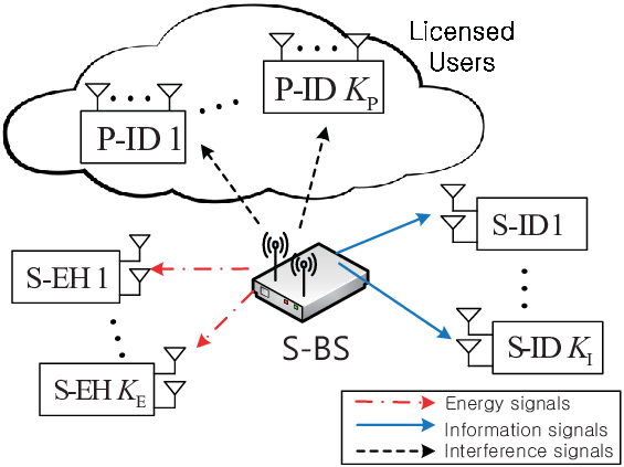
In this paper, we investigate the optimal precoder designs in a general MuMIMO CR SWIPT network, where one secondary base-station (S-BS) supports multiple secondary ID (S-ID) and multiple secondary EH (S-EH) users all having multiple antennas by utilizing the licensed spectrum assigned to the primary ID (P-ID) users as depicted in Fig. 1. We model our transmitter design as a unified framework for sum-utility maximization in the MuMIMO-CR-SWIPT systems, in which the previous studies in [7, 8, 9, 11, 12, 18] are shown to be particular solutions of the proposed framework. The sum-utility maximization problem has initially been proposed in [19] to address different types of cost functions such as the weighted sum-rate (WSR), proportional fairness (PF), and harmonic mean rate (HMR) at once in the conventional MuMIMO systems. However, it remains unclear whether such existing solutions are applicable to the general MuMIMO-CR-SWIPT networks, because the WMMSE transformation techniques in [19] no longer resolve the non-convexity of the original problem even with respect to the precoding matrix only.
A main difference point of our study from the aforementioned previous works is that we treat more general sum-utility maximization problem for the MuMIMO-CR-SWIPT systems, for which the transmit power constraint at the S-BS, the interference power constraint at each P-ID user, and the EH constraint at each EH-user must be satisfied simultaneously. Although the previous work in [18] also considers the CR-SWIPT topology, it is confined to the single S-ID user and a single receive antenna scenarios, which results in an easy-to-solve convex problem. In contrast, our problem is generally non-convex, and thus more challenging to solve. Note that the conventional SDP approach as in [12] is not directly applied to our problem due to the non-linear utility cost functions. To tackle the problem, we demonstrate that the WMMSE problem transformation gives a zero duality gap between the primal and its dual problems. Then, we find the optimal solution by solving the dual problem that is given in the form of non-differentiable convex functions via the sub-gradient ellipsoid method.
The contribution of the paper is summarized as follows.
- •
In Section III, we propose an optimal energy transmission scheme to maximize the amount of energy harvested at the S-EH users under the CR constraints. We first show that the rank- transmission is optimal for maximizing the weighted sum of harvested energy regardless of the number of EH and CR constraints. Then, we propose an efficient algorithm to find the optimal energy beam vector based on the subgradient ellipsoid method. This scheme enables us to identify a feasible range of the energy thresholds in the subsequent precoder designs.
- •
In Section IV, we propose an optimal precoder design for general sum-utility maximization in the MuMIMO-CR-SWIPT networks. First, we prove that the WMMSE problem transformation gives rise to a strong duality in terms of the precoding matrix. Then, we propose an efficient algorithm to find the optimal precoder by adopting the ellipsoid and alternating optimization methods in its inner and outer iterations, respectively. The proposed algorithm converges at least to a locally optimal point, and thus can be made arbitrarily close to the global optimum with the aid of multiple initial points. A modified algorithm is also introduced to address the zero-interference constraints to the primary users.
- •
In Section V, we provide a simplified algorithm that achieves a globally optimal solution considering a special case of the S-BS supporting one S-ID user at a time in a time division multiple access (TDMA) manner, which is called single user MIMO (SuMIMO) CR SWIPT. Unfortunately, the problem is still non-convex. To resolve the problem, we first identify an optimal precoder structure as a closed-form through the Lagrange dual analysis. Then, we propose an efficient algorithm to determine the remaining dual variables based on the subgradient ellipsoid method. The proposed solution finds a globally optimal point without the aid of the alternating optimization and the multiple initial points, and thus is efficient. The solution also can be exploited as a useful outerbound for the MuMIMO-CR-SWIPT system by regarding the multiple S-ID users as a single macro user with ideal multiuser cooperation.
- •
In Section VI, we provide an in-depth discussion on the proposed designs from practical implementation perspectives such as the required CSI at each node, the channel estimation procedure, and the computational complexity.
- •
Finally, in Section VII, we offer extensive simulation results to demonstrate the efficiency of the proposed designs. We first confirm that the proposed SuMIMO design attains the global optimum. Then, we verify the optimality of the MuMIMO design by observing that the performance approaches its SuMIMO outerbound with the aid of multiple initial points. One interesting observation is that the optimal point is achievable with only a few initial points in the low-to-medium SNR region, although a larger number of initial points may be still needed as SNR grows high. Obviously, the proposed MuMIMO design based on the WSR utility achieves the best WSR performance. However, the PF and HMR designs may be preferred over the WSR design in terms of the rate balancing among the S-ID users.
Notations: Throughout the paper, boldface upper and lowercase letters denote matrices and vectors, respectively. The superscripts and stand for the transpose and Hermitian-transpose operations, respectively. We use , , and to denote the expectation, determinant, and trace operations, respectively. The notation represents a blockwise diagonal matrix with matrices . For a matrix , we define , , , and as the largest eigenvalue, the smallest eigenvalue, the element-wise operation, and the gradient of at , respectively. Also, we define as a matrix consisting of ’s from to . We define as an identity matrix. Some important acronyms and notations are summarized in Table I and II, respectively.
| Acronym | Definition |
|---|---|
| CR | Cognitive Radio |
| MMSE | Minimum Mean Squared Error |
| WMMSE | Weighted MMSE |
| MIMO | Multi-input Multi-output |
| MuMIMO | Multiuser MIMO |
| SuMIMO | Single-user MIMO |
| SNR | Signal-to-Noise Ratio |
| WSR | Weighted Sum Rate |
| PF | Proportional Fairness |
| HMR | Harmonic Mean Rate |
| S-BS | Secondary Base Station |
| S-ID | Secondary Information Decoding |
| S-EH | Secondary Energy Harvesting |
| P-ID | Primary Information Decoding |
| CSI | Channel State Information |
II System Model
As shown in Fig. 1, we consider a general MuMIMO-CR-SWIPT network where an unlicensed S-BS with antennas supports S-ID users and S-EH users by sharing the licensed spectrum assigned to the P-ID users such that the performance degradation of each active primary link is within a tolerable margin. It is generally assumed that each of the S-ID, S-EH, and P-ID users has , , and number of antennas, respectively. Here, we assume that is sufficiently large such that to circumvent a feasibility issue for the zero-interference conditions as will be described in more detail in Section IV-C.
Define and as the baseband signal vectors for the data and noise associated with the S-ID users, respectively. Then, considering the narrow-band flat fading channels, the received signal vector for S-ID users can be expressed as
| (1) |
where and denote the channel and the precoding matrices from the S-BS to the S-ID users, respectively. Specifically, we have
where and represent the channel and precoding matrices from the S-BS to the -th S-ID user, respectively. Thus, the received signal at the -th S-ID can be rephrased by
which leads to the information rate to the -th S-ID user as
| (2) |
where denotes the effective noise covariance matrix. For simplicity, here we ignored the interference from the primary transmitter to the S-ID users, but the result can be applied to more general cases. For notational convenience, we also define a stacked noise covariance as .
| Notation | Definition |
|---|---|
| Number of S-BS antennas | |
| Number of antennas at each S-ID user | |
| Number of antennas at each S-EH user | |
| Number of antennas at each P-ID user | |
| Number of S-ID users | |
| Number of S-EH users | |
| Number of P-ID users | |
| Energy threshold at -th S-EH user | |
| Interference threshold at -th P-ID user | |
| Channel between S-BS and -th S-ID user | |
| Channel between S-BS and -th S-EH user | |
| Channel between S-BS and -th P-ID user | |
| Effective noise covariance matrix at -th S-ID user | |
| Precoding matrix for -th S-ID user | |
| Receiver matrix for -th S-ID user | |
| Weight matrix for -th S-ID user | |
| MSE matrix for -th S-ID user | |
Define the downlink channel matrices from the S-BS to the -th S-EH and the -th P-ID users as and , respectively. Then, by employing the conventional linear EH model11 1 Note that the proposed algorithm also works for a practical non-linear EH model as we consider individual EH constraints. Please refer to [20] for more details. in [7], the amount of energy that can be harvested per a unit time at the -th EH-user is quantified as where represents the RF-to-energy conversion efficiency. For ease of presentation, we set unless stated otherwise. Similarly, one can define the total interference power at the -th P-ID user as [4].
We consider the quasi-static fading environment, where the channel matrices are approximately constant over a few transmission blocks. Then, considering the time division duplex (TDD) scheme, the S-BS obtains the channel state information (CSI) of all links utilizing the uplink reference signals from the users, while each S-ID user obtains its own CSI by leveraging the downlink training from the S-BS. Then, we can formulate a precoder design problem for sum-utility maximization in the MuMIMO-CR-SWIPT networks as
where denote the transmit power constraint at the S-BS, and and represent individual harvested energy and interference constraints for the S-EH and P-ID users, respectively. Here, and refer to the target energy level at the -th S-EH user and the target interference level at the -th P-ID user, respectively. indicates a utility function that is for example given by , , and for the WSR, PF, and HMR, respectively. Note that (P-1) is generally non-convex, and thus is difficult to solve in its current form. Throughout the paper, we assume that the S-BS solves (P-1) with global perfect CSIs of . More details about the required CSIs at each node and the corresponding channel acquisition procedure will be discussed later in Section VI.
III Achievable Energy Region
When the EH requirements at the S-EH users grow too high, the system may become infeasible due to limited transmit power at the S-BS. Therefore, it is important to check whether the system is feasible or not before solving the problem in (P-1). In this section, we formulate an weighted sum harvested energy maximization problem in the CR-SWIPT topology to identify the Pareto optimal boundary points of the achievable energy region in (P-1) and provide an efficient algorithm to find a solution.
Let us set as an weight factor for the harvested energy at the -th EH user such that . Then, the weighted sum harvested energy maximization problem can be formulated as
| (P-2) | ||||
| s.t. | ||||
The above problem is convex, for which the strong duality holds. Here, we have relaxed a constraint , but one may recognize from the following proposition that a precoding matrix that is given in the form can achieve the optimal value of (P-2). According to the weight factors ’s, the resulting solution identifies each Pareto optimal boundary point of the achievable energy region.
Proposition 1
With the assumption that , the optimum in (P-2) can be achieved by a rank-1 matrix having full transmit power .
Proof:
First, by contradiction, let us presume that the optimum of (P-2) occurs at a point where . Define an aggregated P-ID user channels . Then, for , we can find a matrix to meet . Therefore, any matrix in the form of with a constant such that achieves a greater amount of energy than without violating all the constraints in (P-2), which contradicts to our previous presumption. Therefore, is always optimal.
In the meantime, let us consider the Lagrangian as
| (3) |
where , , and denote the dual variables corresponding to the S-BS power constraint, the -th CR constraint, and the semi-definite constraint, i.e., , respectively.
Then, from the KKT conditions, we have
| (4) |
where . From the former condition in (4), we have . However, the latter condition, i.e., , only holds for because otherwise becomes a full-rank matrix for which there exists no that satisfies . Therefore, we can conclude that is optimal, which implies that the optimal occurs at a point where all column vectors of are aligned with the eigenvector corresponding to , and the proof is concluded. ∎
The result in Proposition 1 enables us to find a solution of (P-2) without solving the complicated SDP problem. Specifically, let us define . Then, by leveraging (3) and (4), we can formulate a simple dual problem of (P-2) as
where , which is easily solved via the subgradient ellipsoid method [21], for which it can be shown that the subgradient of at a point is given by [22]. Here, denotes the eigenvector of corresponding to . After we find the dual optimal , the primary optimal precoding matrix is computed such that with from Proposition 1. The algorithm is summarized in Table III.
| Initialize . |
| Repeat |
| Compute the subgradient of for a given . |
| Update using the ellipsoid method subject to . |
| Until converges to the prescribed accuracy. |
| Find such that and . |
IV Proposed MuMIMO-CR-SWIPT Precoder Designs
In this section, we provide an efficient optimization algorithm to solve the sum-utility maximization problem in (P-1) for general MuMIMO-CR-SWIPT networks.
IV-A WMMSE Problem Reformulation
First, we transform (P-1) to an equivalent WMMSE problem that is relatively easy to solve. Let us define and as the linear receiver and the final observation at the -th S-ID user, respectively. Then, one can compute the MSE matrix as
| (5) |
where a new variable enables us to obtain an efficient algorithm.
For convenience, let us set for unknown . Then, by introducing an weight matrix , we can reformulate (P-1) to an equivalent WMMSE problem as
where and . Here, denotes the inverse mapping of the gradient map , e.g., . As long as is a strictly concave function for all , the equivalence between (P-1) and (P-4) holds. Detailed proof simply follows from [19, Section II-B].
Although (P-4) is still jointly non-convex, it is now seen as an unconstrained convex problem with respect to each of and for given and . Therefore, the optimal structures of and are easily acquired from the KKT zero-gradient conditions.
Let us set the Lagrangian of (P-4) as
| (6) |
where , , and denote the dual variables corresponding to , the -th , and -th constraints, respectively. Also, here we define and
| (7) | |||||
Then, the KKT necessary conditions for optimality are given by
| (8) | |||
| (9) | |||
| (10) | |||
| (11) | |||
| (12) | |||
| (13) | |||
| (14) | |||
| (15) |
where and . Here, the equations from (8) to (11) stem from the zero gradient conditions with respect to , , , and , respectively, and the equations from (13) to (15) represent the complement slackness conditions. Note that (9) follows from [19, Theorem 2].
IV-B Optimal Precoder Design
Unlike the conventional non-SWIPT designs, (P-4) is still non-convex with respect to and , because the conflicting constraints in , , and form a non-convex feasible domain. Thus, standard CVX tools such as SeDuMi [24] are not immediately applicable even if other variables and are fixed. Therefore, it is most important to determine the optimal structure of and . Once their optimal forms are identified, (P-4) is easily solved by alternately updating , , and until convergence.
First, we observe from (11) that for a fixed , in (6) is expressed as a function of . Thus, we can reduce the number of unknown dual variables by . Also, as we have , at least one variable among has a non-zero positive value, which implies that at least one constraint in and must be activated due to (13) and (15). Thus, for a given , we have
| (18) |
Next, we consider a Lagrange dual function of (P-4) as
| (19) |
where is obtained by applying (11) to (6) as
| (20) |
Here, we define and . Now, let us temporarily ignore the constant terms in with respect to , which makes (19) rephrased by
| (21) |
where with . Now, suppose that at least one eigenvalue of is non-positive with corresponding eigenvector . Then, we can make (21) unbounded from below by simply setting with . Therefore, a dual feasible condition arises for (19), which leads us to the following dual problem as
Proposition 2
There exists zero-duality gap between (P-4) and its dual (P-5) with respect to and .
Proof:
See Appendix -A. ∎
With the assistance of Proposition 2, we can find optimal through (P-5) that is solvable via the ellipsoid method for constrained problems [21], for which the subgradient of at a feasible point is computed by . Here, denotes the corresponding primal optimal solution. Note that is invertible for a feasible since , and thus we have
Otherwise if violates the dual feasible condition, i.e., , we compute the subgradient of as where represents the eigenvector of corresponding to . The algorithm is summarized in Table IV. After finding the optimal , we finally set as in (18), which results in the optimal precoder .
| Initialize . |
|---|
| Repeat |
| Compute for a given . |
| if |
| Compute . |
| Compute the subgradient of . |
| else |
| Compute the subgradient of . |
| end |
| Update using the ellipsoid method subject to . |
| Until converges to the prescribed accuracy. |
| Set . |
Algorithm 1 illustrates the entire WMMSE algorithm for sum-utility maximization in general MuMIMO CR SWIPT systems with S-ID, S-EH, and P-ID users. The algorithm converges, since each update of , , and minimizes the weighted sum-MSE that is bounded from below. The converged point ensures the local optimum because all gradients with respect to , , and simultaneously vanish. Nevertheless, due to jointly non-convexity of (P-4), we may need different random initial points so that the resulting local minimum gets closer to the global minimum. This may require additional outer-loop iterations.
IV-C Zero-interference Design
When for some where denotes a subset of P-ID user indices , the algorithm in Section IV may be inefficient and unstable, because we may find unnecessary dual variables that are associated with the zero-interference constraints. It is thus imperative to modify the optimization problem so that one can solve the problem more efficiently.
Define a stacked P-ID user channel matrix as
| (22) |
where designates a cardinality of . As we assume that , we can also define a matrix whose column vectors constitute the orthonormal basis in the null-space of , i.e., with . Note that otherwise if , the system might be infeasible.
The precoding matrix that satisfies the zero-interference constraints, i.e., , must be in the null-space of . Therefore, without loss of optimality, the optimal precoder can be generally expressed by for any matrix . Thus, applying the result to (P-1), we obtain a modified optimization problem as
where denotes a complementary set of and with , , and . Once we find , the resulting solution achieves the zero interference constraints, i.e., with reduced number of dual variables by , and thus is efficient. The rest of derivations is the same as the previous section. Note that when we consider all zero interference, i.e., , the CR constraints in (P-6) is completely removed, which we call a zero-forcing (ZF) design. Further, if we have and , (P-6) becomes equivalent to the one in [9].
V Joint Optimal Solution for Single S-ID User
In practice, the S-BS may support one S-ID user at a time in a TDMA manner. In this case, our system model reduces to the SuMIMO channel with multiple CR and EH constraints, for which we can show that the WMMSE problem in (P-4) can be jointly optimized without the aid of the multiple initial points and the alternating optimization among the filters. The result in this section not only provides the globally optimal solution for the SuMIMO-CR-SWIPT system, but also serves as a theoretical performance outer bound for the MuMIMO-CR-SWIPT systems in the previous section. Throughout the section, we will drop the S-ID user index from all variables related to the S-ID users, since we only consider . Also, the auxiliary variable in (5) is now included in the receiver from the joint optimization perspective.
V-A Joint Optimal Precoder Design
Setting and , and plugging (16) into (P-4), we obtain a modified WMMSE problem for as
where , , and
| (23) | |||||
Here, (23) follows, since for the general sum-utility maximization in (P-1) boils down to the rate maximization, i.e., , for which the inverse mapping of is explicitly given by . Note that (P-7) is still jointly non-convex, and therefore the optimal solution is not immediate from there.
Define the Lagrangian for (P-7) as
| (24) |
with . We first see from (24) that the optimal weight matrix for a given should be positive definite, because we have
| (25) | |||||
| (26) |
where (25) follows from the optimality condition in (17). Based on the result, now we can find the optimal precoding structure as described in the following proposition.
Proposition 3
The optimal solution in (P-7) for a given positive definite weight matrix has the form of
| (27) |
where and come from the following eigenvalue decomposition
| (28) |
with a unitary matrix and a square diagonal matrix having the eigenvalues of (28) in a descending order.
Proof:
See Appendix -B. ∎
V-B Weight Matrix Design
The weight matrix can be designed differently according to the applications.
V-B1 Maximum Rate Design
Due to the equivalence between (P-1) and (P-7), the maximum rate can be achieved when both and jointly solve (P-7). To this end, the optimal weight matrix must satisfy the equality in (26) that is alternatively expressed by using in (27) as
| (29) |
Thus, the -th diagonal element of should become
where denotes the -th diagonal element of . It is seen from (27) that when and , the -th data stream will be unused. As a result, without loss of optimality, we can set the maximum rate precoder as
| (33) |
V-B2 Quality of Service (QoS) Design
For any given weight factors, the precoder in (27) minimizes the weighted sum-MSE, i.e., in (P-7). Therefore, besides the rate maximization, the solution can be exploited for handling the error performance of each data stream so as to ensure the QoS.
Specifically, the QoS design can be achieved by setting and applying the unitary discrete Fourier transform (DFT) matrix to (27) as
| (34) |
Here, we notify that the DFT matrix enables all the MSEs, i.e., the diagonal elements of the MSE matrix in (P-7), have the same value without changing their sum [23] [9]. Since we have , the resulting solution minimizes the maximum MSE among data streams while maintaining the minimum sum-MSE, thereby achieving the QoS. The QoS design is particularly useful when independent messages are spatially multiplexed across the sub-channels and should be separately decoded. Note that for the case of a singe S-ID user with a single antenna, i.e., , the two solutions in (33) and (34) are merged into one. Further, if , they reduce to the CR-SWIPT beamforming scheme in [15].
V-C Dual Variable Optimization
The remaining problem is to determine the dual variables in (27). Let us consider the dual problem constrained by the dual feasibility (see (35) in Appendix -B) as
Then, following the same argument in Proposition 2, we can show that the strong duality holds between (P-7) and its dual (P-8). Therefore, the optimal dual variables in (27) can be attained by solving (P-8), which is accomplished by applying the ellipsoid method, for which the subgradient of at a feasible point is computed by . Otherwise if is infeasible, i.e., , we update utilizing the subgradient of as , where denotes the eigenvector of corresponding to . The ellipsoid updating procedure is summarized below. The algorithm finds the global optimal solution of (P-7) attributed to the strong duality of (P-7) and (P-8) as proved in Proposition 2, the primal optimal solution in Proposition 3, and the convexity of (P-8) for which the ellipsoid algorithm converges to the dual optimum [21].
VI Discussion
In this section, we provide an in-depth discussion on the proposed precoder designs from a practical implementation perspective. First, we investigate the amount of CSIs required at each secondary node and the channel estimation procedures for it. Then, we also quantify the computational complexity of the proposed algorithms to get more insight into the design.
VI-A Required CSIs at Each Node
In order to meet all required constraints in the CR-SWIPT networks, the S-BS must control the secondary users with global CSIs of . Therefore, it is reasonable to assume that the precoding matrix is computed at the S-BS. In contrast, the S-ID users do not need to compute , because only the information of effective downlink channel and noise covariance is sufficient for the -th S-ID user to decode its own message as shown in (2). The S-EH users require neither the precoding matrix nor the CSI, since no further receive signal processing is needed for energy harvesting. Note that there is no required CSI at the primary nodes to do with the secondary network.
VI-B Channel Acquisition Procedure
To achieve the potential benefits of the proposed precoder designs, an accurate channel estimation at the S-BS is essential. Thus, for channel estimation, the time division duplexing (TDD) scheme that can exploit the channel reciprocity between a transmitter and a receiver is a better choice than the frequency division duplexing scheme. In this subsection, we introduce TDD based channel acquisition processes to achieve the required CSIs at each node.
First, in the beginning of each channel coherence block, the secondary users transmit orthogonal training sequences to the S-BS to allow the S-BS to estimate the CSIs of both and . Note that the pilot transmission of the S-EH users is also achievable by using the energy stored in their own batteries or the energy that has been harvested in the previous transmission frame [25]. The S-BS also estimates the P-ID user channels by listening to the periodic uplink pilots transmitted from the P-ID users to the primary transmitter [2, 3, 4]. With the acquired CSIs, the S-BS is now able to compute the precoding matrix through Algorithm 1 or 2.
Next, during the downlink training phase, the -th S-ID can estimate the effective downlink channel by utilizing the precoded training sequences at the S-BS. For example, the demodulation reference signaling in long-term evolution advanced (LTE-A) can be employed [26]. Then, the S-BS feedforwards the effective noise covariance to each -th S-ID user through the downlink control channels.22 2 It is also possible for each S-ID user to apply the blind noise estimation scheme [27] to estimate its own effective noise.
VI-C Complexity Analysis
| Algorithm 1 | Algorithm 2 | |
| - | ||
| - | ||
| - | ||
| - | ||
| - | ||
| - | ||
| [21] | ||
| Total | ||
In what follows, we briefly examine the computational complexity of the proposed algorithms. As it is hard to measure the exact amount of computations, we instead calculate the order of floating point operations required to find the optimal precoder at the S-BS. Based on the analysis of matrix computation complexity in [22], the computational complexity of the proposed algorithms is analyzed in Table III.
The result of complexity analysis is summarized in Table V. Here, represents the required complexity for computing operation set , and and denote the required number of iterations for the ellipsoid and alternating optimization process, respectively.
First, the result confirms that the SuMIMO design in Algorithm 2 indeed obtains complexity advantage over the MuMIMO design in Algorithm 1 for the case of , because the multiple initial points and the alternating optimization process are unnecessary, not to mention the additional efforts for computing the auxiliary filter matrices, i.e., . One interesting observation is that the amount of computations for Algorithms 1 and 2 increases in the orders of and , respectively. This means that the complexity gain of Algorithm 2 will be more pronounced as the S-ID user antenna grows,
However, it should be noted that as and increase, the MuMIMO design that can support multiple S-ID users at the same time and frequency attains a significant throughput gain over the SuMIMO design based on the scheduling. Therefore, Algorithm 1 is also important for achieving high data throughput in multiuser scenarios. A careful examination on Table V reveals that the entire complexity for Algorithm 1 is mostly influenced by the number of antennas of the S-BS and the S-ID users, i.e., and as in the conventional non-SWIPT or non-CR MuMIMO systems [3] [9] [19]. Therefore, computational complexity of the proposed designs is comparable with those in the conventional systems.
VII Numerical Results
| Parameter | Value |
|---|---|
| Noise Power Spectral Density | dBm/Hz |
| Signal Bandwidth | MHz |
| Energy Conversion Efficiency | () |
| Channel Model | Rayleigh pathloss model |
| Pathloss Exponent | |
| User Distance from S-BS | m |
| Reference Distance | m |
| Transmit Power () | dBm |
In this section, we demonstrate the efficiency of the proposed algorithms for MuMIMO-CR-SWIPT networks through the numerical results. For our simulations, we have chosen the system parameters as in Table VI.33 3 We have set the parameters such that the average received signal power at each secondary user appears in a common SNR range, e.g., dB. However, it should be noted that the proposed scheme is universally applicable to any system parameters. For ease of presentation, we assume that all the S-ID, S-EH, and P-ID users are located in the same distance from the S-BS. Then, considering the Rayleigh pathloss model with the parameters in Table VI, we can construct the channel matrices as , , and , where , , and denote random matrices whose entries are drawn from independent and identically distributed standard complex Gaussian. We consider the same noise power at all S-ID users being equal to dBm and the same interference threshold for all P-ID users, i.e., .44 4 Throughout the section, we set the interference thresholds such that they appear between and a certain positive value which is smaller than the maximum interference level that can be met by a non-CR SWIPT design considering no CR constraints. Similarly, the energy thresholds and are set to be in the feasible energy region, while being greater than the minimum energy level that is automatically achievable by a non-SWIPT CR design considering no EH constraints. We use an initial value for (P-3). The initial values of (P-5) and (P-8) are similarly defined. We adopt random initial points for Algorithm 1 unless specified otherwise. For simplicity, we set for the WSR design.

In Figs. 2 and 3, we investigate the SuMIMO-CR-SWIPT networks with . Fig. 2 illustrates the convergence trend of Algorithm 1 and 2 for a system with and W. Interestingly, we see that a few initial points may be sufficient for Algorithm 1 in dBm to achieve the maximum rate, while a number of initial points may be needed in dBm. The result implies that although the WMMSE cost function in (P-4) may have a convex-like form in the low SNR region, it becomes highly non-convex as SNR goes to high. Despite the non-convexity of (P-4), we confirm that Algorithm 2 achieves the global optimum with a single initial point even without the alternating optimization process, and thus is efficient.

In the meantime, Fig. 3 presents the convergence trend of the ellipsoid process in Algorithm 2 in terms of the sum-MSE performance for a system with W. We observe that the QoS design in (34) achieves the minimum sum-MSE in contrast to the max-rate design. Further, the QoS design makes all sub-channels experience the same MSE. Therefore, the MSE gain of the QoS design leads to the bit error rate performance advantage over the max-rate design [23]. Observe that as the interference threshold becomes tighter, the convergence speed gets slower. The result shows that when , the system could be inefficient, for which the zero-interference design in Section IV-C becomes useful.


Figs. 4 and 5 consider the MuMIMO-CR-SWIPT systems for a system with and dBm, and show the rate-energy tradeoff performance in a 3-D plot and in its 2-D intersection at W, respectively. Here, we employed the WSR utility as an objective function of (P-1) to acquire the maximum WSR. The name of “SuMIMO outerbound” amounts to the case of perfect collaboration among the multiple S-ID users, which results in a single macro S-ID user with . Unlike the case of , it is generally difficult to identify whether the resulting solution is optimal or not due to the lack of knowledge on the global optimal solution. Nevertheless, we can carefully infer that the proposed solution achieves the optimal boundary points based on the observation that all the tradeoff regions exhibit a nice convex shape and are close to their single-user outer bounds. At any information rate, there exists an unachievable energy region, which shows that the feasibility check in Section III is important before solving the problem. Obviously, as decreases, the achievable tradeoff region will shrink to meet tighter CR constraints. One interesting observation in Fig. 5 is that as the energy threshold approaches its maximum value, the achievable rate converges to its outerbound. This confirms our previous statement in Proposition 1 that the maximum energy of an S-EH user is achievable via a single beam vector that is pointing in one direction irrespective of the S-ID user topology.

Fig. 6 shows a snapshot of the ellipsoid process in Algorithm 1 in terms of the harvested energy and the interference power for a system with and . Here, we set the threshold values as W, W and W. The figure confirms that the proposed algorithm achieves all the required constraints. The interference power is kept below the threshold attributed to the power normalizing factor in (18).

In Fig. 7, we plot the WSR performance of various precoder designs in systems with , , and dBm. For a fair comparison, we introduce the round robin scheduling or opportunistic max-user selection schemes [28] to the SuMIMO design. As expected, as increases, the proposed MuMIMO designs that can support multiple S-ID users simultaneously attain significant performance advantage over the SuMIMO design based on the scheduling, although the SuMIMO design attains complexity gain for the case of a single S-ID user. The gain grows larger as and increases.


In Fig. 8, we compare the rate balancing performance of various MuMIMO precoder designs for a system with , , , and dBm. Obviously, the WSR design achieves the best sum-rate performance. However, the PF and HMR designs may be more attractive in terms of the worst user rate or fairness. It is observed that the HMR design yields the best balance among the S-ID users at the cost of slight sum-rate performance loss.
Similar observation can be made in Fig. 9 which exhibits both the sum-rate and minimum user-rate performance for a system with , , and dBm. Here, “WSR-ZF design” denotes the WSR solution that is obtained from (P-6) with and . We observe that although the ZF design may provide a simpler solution, it cannot achieve an additional performance gain from both the sum-rate and minimum user rate points of view in a situation where some amount of interference is allowable. This highlights the interference control capability of the proposed MuMIMO-CR-SWIPT designs. As becomes smaller, the performance variation among the different utility functions diminishes. This is because the degree of freedom of the precoder design is constrained within the null space of the P-ID user channels .
VIII Conclusion
In this paper, we have investigated the optimal precoder designs for general sum-utility maximization in the MuMIMO-CR-SWIPT networks. First, we examined the optimal energy transmission scheme to identify the feasible energy region. Second, we proposed an efficient algorithm to find the optimal MuMIMO precoders by adopting the ellipsoid and alternating optimization process, for which multiple initial points may be necessary to approach the global optimum. Then, we suggested a simplified algorithm that can find a globally optimal solution without resorting to the alternating optimization as well as the multiple initial points in a special case of a single S-ID user. We also have offered an in-depth discussion on the proposed designs in terms of the computational complexity and the channel information requirement. Finally, we verified the efficiency of the proposed designs via numerical simulation results. An investigation on the tradeoff between the training phase duration and channel estimation accuracy in the imperfect CSI scenarios will be an interesting topic for future works.
-A Proof of Proposition 2
Let , , and be any points that satisfy the KKT and dual feasible conditions. Define the objective function of (P-4) as . Then, by the weak duality theorem [24], one can show that
Here, the second line follows from (19) and the third line is due to the fact that is convex in under the dual feasible condition , which means that the infimum of occurs at a point where its gradient vanishes, i.e., . In the last line, we use the complementary slackness conditions in (13)-(15). Thus, we can conclude that , and the proof is completed.
-B Proof of Proposition 3
For any optimal and an arbitrary unitary matrix , we can always find a modified solution that is also optimal, since we have
Here, we can choose such that is diagonalized without loss of optimality. In this case, the off-diagonal elements in will not affect the first term of (24). In addition, by the Hadamard’s inequality , we have with being the -th diagoanl element of . Therefore, we see that a diagonal weight matrix suffices to achieve the minimum of (24).
Next, let us define a vector of the dual variables in (24) as . Then, a dual feasible condition arises for , because otherwise the corresponding dual function goes to where
| (35) |
Under the dual feasibility, is invertible, which means that one can generally express the optimal precoder as for any matrix .
Since is full-rank, there are at most number of non-zero eigenvalues in . Let us further develop as where and are the associated sub-matrices of . Then, it is true that since it only increases in (24), which leads to
| (36) |
Lastly, by substituting in (24) with (36), we obtain a modified Lagrangian as
| (37) |
Now, we can verify from Lemma 1 and 2 below that the Lagrangian in (37) touches its minimal point when forms a diagonal matrix because in this case in (26) is given by a diagonal matrix and the first and third terms of (37) can be simultaneously minimized. Then, becomes convex with respect to where denotes the -th diagonal element of . Thus, by setting , we obtain with being the -th diagonal element of . Finally, we have
Lemma 1 ([22])
For any square matrix , it is true that where stands for the -th diagonal element of .
Lemma 2 ([29])
For any positive definite matrix , we have where stands for the -th diagonal element of .
References
- [1] M. Gastpar, “On capacity under receive and spatial spectrum-sharing constraints,” IEEE Trans. Inf. Theory, vol. 53, no.2, pp. 471–487, Feb. 2007.
- [2] R. Zhang and Y. C. Liang, “Exploiting multi-antennas for opportunistic spectrum sharing in cognitive radio networks,” IEEE J. Sel. Topics Signal Process., vol. 2, no.1, pp. 88–102, Feb. 2008.
- [3] R. Zhang, Y. C. Liang, and S. Cui, “Dynamic resource allocation in cognitive radio networks,” IEEE Signal Process. Mag., vol. 27, no.3, pp. 102–114, May 2010.
- [4] K.-J. Lee and I. Lee, “MMSE based block diagonalization for cognitive radio MIMO broadcast channels,” IEEE Trans. Wireless Commun., vol. 10, no.10, pp. 3139–3144, Oct. 2011.
- [5] X. Lu, “Wireless networks with RF energy harvesting: A contemporary survey,” IEEE Commun. Surveys Tuts, vol. 17, no.2, pp. 757–789, Apr. 2015.
- [6] S. Bi, C. K. Ho, and R. Zhang, “Wireless powered communication: Opportunities and challenges,” IEEE Commun. Mag., pp. 117–125, Apr. 2015.
- [7] R. Zhang and C. K. Ho, “MIMO broadcasting for simultaneous wireless information and power transfer,” IEEE Trans. Wireless Commun., vol. 12, no.5, pp. 1989–2001, May 2013.
- [8] C. Song, C. Ling, J. Park, and B. Clerckx, “MIMO broadcasting for simultaneous wireless information and power transfer: Weighted MMSE approaches,” in Proc. IEEE GLOBECOM Workshops, pp. 1151–1156, Dec. 2014.
- [9] C. Song, J. Park, B. Clerckx, I. Lee, and K.-J. Lee, “Generalized precoder designs based on weighted MMSE criterion for energy harvesting constrained MIMO and multi-user MIMO channels,” IEEE Trans. Wireless Commun., vol. 15, no.12, pp. 7941–7954, Dec. 2016.
- [10] C. Song and Y. Jeon, “Weighted MMSE precoder designs for sum-utility maximization in multi-user SWIPT network-MIMO with Per-BS power constraints,” IEEE Trans. Veh. Technol., vol. 67, no.3, pp. 2809–2813, Mar. 2018.
- [11] J. Xu, L. Liu, and R. Zhang, “Multiuser MISO Beamforming for Simultaneous Wireless Information and Power Transfer,” IEEE Trans. Signal Process., vol. 62, no.18, pp. 4798–4810, Aug. 2014.
- [12] J. Rubio, A. P. Iserte, D. P. Palomar, and A. Goldsmith, “Joint opimization of power and data transfer in multiuser MIMO systems,” IEEE Trans. Signal Process., vol. 65, no.1, pp. 212–227, Jan. 2017.
- [13] Z. Zhu, Z. Chu, Z. Wang, and I. Lee, “Outage constrained robust beamforming for secure broadcasting systems with energy harvesting,” IEEE Trans. Wireless Commun., vol. 15, no.11, pp. 7610–7620, Nov. 2016.
- [14] Z. Zhu, Z. Chu, N. Wang, S. Huang, Z. Wang, and I. Lee, “Beamforming and power splitting designs for AN-aided secure multi-user MIMO SWIPT systems,” IEEE Trans. Inf. Forensics Security, vol. 12, no.12, pp. 2861–2874, Dec. 2017.
- [15] Z. Zhu, Z. Chu, F. Zhou, H. Niu, Z. Wang, and I. Lee, “Secure beamforming designs for secrecy MIMO SWIPT systems,” IEEE Wireless Commun. Lett., vol. 7, no.3, pp. 424–427, Jun. 2018.
- [16] H. Lee, C. Song, S.-H. Choi, and I. Lee, “Outage probability analysis and power splitter designs for SWIPT relaying systems with direct link,” IEEE Commun. Lett., vol. 21, no.3, pp. 648 – 651, Mar. 2017.
- [17] Z. Zong, H. Feng, F. R. Yu, N. Zhao, T. Yang, and B. Hu, “Optimal transceiver design for SWIPT in K-user MIMO interference channels,” IEEE Trans. Wireless Commun., vol. 15, no.1, pp. 430–445, Jan. 2016.
- [18] F. Zhu, F. Gao, and M. Yao, “A new cognitive radio strategy for SWIPT system,” in International Workshop on High Mobility Wireless Communications, pp. 73–77, 2014.
- [19] Q. Shi, M. Razaviyayn, Z.-Q. Luo, and C. He, “An iteratively weighted MMSE approach to distributed sum-utility maximization for a MIMO interfering broadcast channel,” IEEE Trans. Signal Process., vol. 59, no.9, pp. 4331–4340, Sept. 2011.
- [20] E. Boshkovska, D. W. K. Ng, N. Zlatanov, and R. Schober, “Practical non-linear energy harvesting model and resource allocation for SWIPT systems,” IEEE Commun. Lett., vol. 19, no.12, pp. 2082–2085, 2015.
- [21] S. Boyd, Ellipsoid Methods. Notes for EE364b, Stanford University, 2018.
- [22] G. H. Golub and C. F. V. Loan, Matrix Computations. Third Edition, The Johns Hopkins University Press, Baltimore and London, 1996.
- [23] D. P. Palomar, J. M. Cioffi, and M. A. Lagunas, “Joint Tx-Rx beamforming design for multicarrier MIMO channels: a unified framework for convex optimization,” IEEE Trans. Signal Process., vol. 51, no.9, pp. 2381–2401, Sept. 2003.
- [24] S. Boyd and L. Vandenberghe, Convex Optimization. The Edinburgh Building, Cambridge: Cambridge University Press, 2004.
- [25] H. Ju, C. K. Ho, R. Zhang, and Y. L. Guan, “Throughput optimization for massive MIMO systems powered by wireless energy transfer,” IEEE J. Sel. Areas Commun., vol. 33, no.8, pp. 1640–1650, Aug. 2015.
- [26] E. Dahlman, S. Parkvall, J. Skold, and P. Beming, LTE / LTE-advanced for mobile broadband. Linacre House, Jordan Hill, Oxford: Elsevier Ltd., 2014.
- [27] M. Frikel, W. Utschick, and J. Nossek, “Blind noise and channel estimation,” in Proc. IEEE Statistical Signal and Array Processing Workshop, pp. 141–145, Aug. 2000.
- [28] A. Asadi and V. Mancuso, “A survey on opportunistic scheduling in wireless communications,” IEEE Commun. Surveys Tuts., vol. 15, no.5, pp. 1671–1688, Fourth Quater 2013.
- [29] N. Komaroff, “Bounds on eigenvalues of matrix products with an application to the algebraic riccati equation,” IEEE Trans. Autom. Control, vol. 35, no.3, pp. 348–350, Mar. 1990.