Experimental Cryptographic Verification for Near-Term Quantum Cloud Computing
Abstract
Recently, there are more and more organizations offering quantum-cloud services, where any client can access a quantum computer remotely through the internet. In the near future, these cloud servers may claim to offer quantum computing power out of reach of classical devices. An important task is to make sure that there is a real quantum computer running, instead of a simulation by a classical device. Here we explore the applicability of a cryptographic verification scheme that avoids the need of implementing a full quantum algorithm or requiring the clients to communicate with quantum resources. In this scheme, the client encodes a secret string in a scrambled IQP (instantaneous quantum polynomial) circuit sent to the quantum cloud in the form of classical message, and verify the computation by checking the probability bias of a class of output strings generated by the server. We provided a theoretical extension and implemented the scheme on a 5-qubit NMR quantum processor in the laboratory and a 5-qubit and 16-qubit processors of the IBM quantum cloud. We found that the experimental results of the NMR processor can be verified by the scheme with about error, after noise compensation by standard techniques. However, the fidelity of the IBM quantum cloud is currently too low to pass the test (about error). This verification scheme shall become practical when servers claim to offer quantum-computing resources that can achieve quantum supremacy.
Introduction.— Quantum computation promises a regime with unprecedented computational power over classical devices, offering numerous interesting applications, such as factorization [1], quantum simulation [2, 3], and quantum machine learning [4, 5]. However, before quantum computers become prevalent to the public, one might expect that only organizations with sufficient resources could operate a full-scale quantum computer, analogous to today’s supercomputers. Furthermore, individuals who have demands for quantum computation could access the service through the internet, i.e., cloud quantum computing. In fact, several small-scale quantum cloud services have already been launched [6, 7, 8], which can be operated by remote clients through the internet. As a result, many simulations performed from quantum cloud servers have been reported (see Ref. [9] for a summary).
In the near future, it is not impossible that these clouds may claim to offer 100 or more working qubits and many layers of quantum gates, where quantum supremacy [10, 11, 12, 13] could be achieved. However, one may naturally ask, is there a real quantum computer behind the cloud? Or, would it just be a classical computer simulating quantum computation? For ordinary clients who only have control and access of classical computer, a natural task is to verify whether these cloud servers are truly quantum.
Alternatively, the question can be formalized as follows: is it possible for a purely-classical client to verify the output of a quantum prover? This question has been extensively explored for more than ten years. In 2004, Gottesman initialized this question, which Aaronson wrote down in his blog [14]. A straight-forward idea is to run a quantum algorithm solving certain NP problems, for example, Shor’s algorithm for integer factorization [1]. Such problems might be hard for classical computation, but are easy for classical verification once the result is known. However, the challenge is that a full quantum algorithm typically requires thousands of qubits and quantum error correction to be implemented, which is out of question in the NISQ [15] (Noisy Intermediate-Scale Quantum) era.
Note that the verification problem have different variants. For example, one may assume that the supposedly “classical” client may actually have a limited ability to perform quantum operations on a small number of qubits. This line of research has already attracted much attention [16, 17, 18, 19, 20, 21, 22]. Without any quantum power, the client might still be able to verify delegated quantum computation which is spatially separated and entanglement can be shared [23, 24]. Currently, this approach does not seem to fit the setting of the available quantum cloud services, but it does reveal the outstanding challenge for establishing a rigorous verification scheme based on a classical client interacting with a single server using only classical communication [25].
Until recently, Mahadev has made important progresses [26, 27], assuming that the learning-with-errors problem [28] is computationally hard even for quantum computer. The protocol allows a classical computer to interactively verify the results of an efficient quantum computation, achieving a fully-homomorphic encryption scheme for quantum circuits with classical keys. Despite these great efforts, we are still facing the problems of “non-interactively” verifying near-term quantum clouds, which would be too noisy for implementing full quantum algorithms but may be capable of demonstrating quantum supremacy.
Here we report an experimental demonstration of a simple but powerful cryptographic verification protocol, originally proposed by Bremner and Shepherd [29] in 2008. We extended the theoretical construction in terms of -point correlation. The implementation was first performed with a 5-qubit NMR quantum processor in the laboratory. Additionally, we also benchmarked the performance of the verification scheme by actually implementing the protocol with the IBM quantum cloud processors [6].
The verification protocol implemented is based on a simplified circuit model of quantum computation, called IQP (instantaneous quantum polynomial) model [29]; the qubits are always initialized in the ‘0’ state. The IQP circuits contain three parts. In the first and the last part, single-qubit Hadamard gates are applied to every qubit. The middle part of an IQP circuit does not contain an explicit temporal structure, in the sense that diagonal (and hence commuting) gates acting on single or multiple qubits are applied. On one hand, the IQP model represents a relatively resource-friendly computational model to be tested with near-term quantum devices. On the other hand, the IQP model has been proven to be hard for classical simulation [30, 31], under certain computational assumptions, similar to Boson sampling [32].
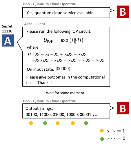
Verification protocol.— In the cryptographic verification protocol [29], there are two parties labeled as Alice (the client) and Bob (the server). Alice is assumed to be completely classical; she can only communicate with others through classical communication (e.g., internet). Suppose Bob claims to own a quantum computer and Alice is going to test it. In reality, of course, there is no need for Alice to inform Bob about her intention; she may just pretend to run a normal quantum program. The protocol can be succinctly summarized as follows (depicted by Fig. 1).
- Step 1:
Alice first generates a matrix (called X-program [29]) associated with a secret string , which is only kept by Alice.
- Step 2:
Alice then translates the X-program into an IQP circuit of qubits, and sends the information about the IQP circuit to Bob.
- Step 3:
Bob returns the outputs to Alice in terms of the bit strings , which should follow the distribution of the IQP circuit, i.e., , if Bob is honest.
- Step 4:
Ideally, Alice should be able to determine if the probability distributions for a subset of strings orthogonal to the secret string, where , add up to an expected value 0.854. Otherwise, Bob fails to pass the test.
More specifically, the key quantity of interest is the following probability bias defined by,
| (1) |
where if it is true that , and otherwise. For a perfect quantum computation, the value of the probability bias should be . The best known classical algorithm [29] would instead produce a value of 0.75, which is relevant when is sufficiently large. This quantum-classical gap in the probability bias makes it possible to apply such a resource-friendly cryptographic verification scheme for testing quantum cloud computing in the regime where quantum supremacy would be achieved.
Overview.— To illustrate our experimental demonstrations, we shall first provide a concise and self-contained theoretical description of the cryptographic protocol. Particularly, our computer code implemented in the experiment is open source and available online [33] and in Supplemental Materials; interested readers can readily reproduce our results with it, and can also apply it to generate X-programs of different variations for testing other quantum-cloud services.
On the other hand, we also provide a theoretical extension of the original work [29], transforming it into a form more familiar to the physics community. Specifically, we connect the probability bias in Eq. (1) with the Fourier coefficient of the probability of the output strings. As a result, we can express the probability bias through the -point correlation function (see Supplemental Materials):
| (2) |
Since the string is not known to Bob, the verification protocol can be regarded as a game where Alice tests the outcomes in terms of a particular correlation function unknown to Bob.
In addition, as we will see later, the X-program consists of two part, the main part and the redundant parts, and the representation of Eq. (2) provides a straight-forward way to understand why the redundant part of the X-program does not affect the probability bias—they commute with the -point correlation function.
Our theoretical extension in Eq. (2) allows us to take into account the effect of noises. More precisely, if one models [34, 35] the decoherence by a dephasing channel (with an error rate ) applied for each qubit at each time step, then the probability bias becomes , where is the Hamming weight of , that is the number of 1’s in .
Experimentally, our data were taken separately from two different sources, namely a five-qubit NMR processor in the laboratory, and the IBM cloud services, aiming to benchmark the performances of the IQP circuit implementation under the laboratory conditions and that from the quantum-cloud service.
Our results show that the laboratory NMR quantum processor can be employed to verify the IQP circuit after noise compensation by standard techniques, but the IBM quantum cloud was too noisy. The probability bias obtained from the IBM’s processors are close to 0.5, which is the result of uniform distribution. The main reason is that IBM’s system has many constraints on the connectivity between the physical qubits; we had to include many extra SWAP gates to complete the circuit, causing a severe decoherence problem.
Theoretical construction.— Here Alice’s secret vector of string is given by . An X-program can be represented by a matrix with binary values, which is constructed from the quadratic residue code (QRC) [36]. In the experiment, the matrix associated with the X-program is given by the following (see Supplemental Material for the construction method),
Here the X-program has a layer of security for protecting the knowledge of the secret string from Bob. Explicitly, there are two parts in the matrix, (i) the main part and (ii) a redundant part. Columns in the main part are not orthogonal to the secret vector , i.e., , while columns in the redundant part are, i.e., . Both parts have to be changed if the secret string is changed.
However, an important property of the X-program is that the probability bias depends only on the main part. So Alice can append as many redundant columns that are orthogonal to to this matrix as she wishes. Of course, later she would need to scramble the columns, in order to hide the secret from Bob.
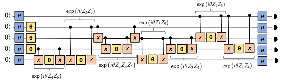
Next, the X-program has to be translated into an IQP circuit [29], which is a subclass of quantum circuits with commuting gates before and after the Hadamard gates. Equivalently, the unitary transformation associated with the IQP circuit can be casted as follows:
| (13) |
where , and is the effective Hamiltonian constructed by the elements of the X-program. For example, a column represents a term , where is a Pauli- acting on the -th qubit. As a result, the full Hamiltonian corresponding to reads,
| (14) |
Note that if we take , then the evolution can be simulated classically by the Gottesman-Knill algorithm [37]. Fig. 2 shows the circuit diagram.
In the ideal case, the probability bias for the IQP circuit should be given by . If Bob outputs random bits, the value of the probability bias would be . However, although it is scrambled, the X-program is correlated with the secret string. The classical algorithm provided in Ref. [29] can yield , which was conjectured to be optimal [29]. As a result, it becomes possible to verify the quantum hardware behind the quantum clouds by simply collecting the statistics of the outputs to check if we can get .
For the purpose of benchmarking, we performed a total of three separate implementations of the same X-program on an NMR quantum processor and on IBM quantum processors, including the 5-qubit one and the 16-qubit one [6].
Verification with NMR in the laboratory.— The experiments with the NMR quantum processor were carried on a Bruker AV-400 spectrometer at 303K. The 5-qubit quantum processor consists of two nuclear spins and three nuclear spins in 1-bromo-2,4,5-trifluorobenzene dissolved in the liquid crystal N-(4-methoxybenzylidene)-4-butylaniline (MBBA) [38]. The molecular structure and equilibrium spectra of nuclear spins are provided in the Supplemental Materials.
Starting from the thermal state , the NMR system is initially prepared in a PPS by the line-selective method [39]. Here represents the identity operator and is the polarization. Note that the identity operator is invariant under the unitary transformation, neither does it affect the measurement step. The state evolves the same way as a true pure state and generates the same signal up to a proportionality factor , so we can simply regard the as .
To implement the IQP circuit, i.e. the described by Eq. (13), we packed it into one shaped pulse optimized by the gradient ascent pulse engineering (GRAPE) method [40], with the length being 37.5 ms and the number of segments being 1500. The shaped pulse has the theoretical fidelity of and is designed to be robust against the inhomogeneity of the pulse amplitude.
To obtain the probability bias in the experiment, we need five readout pulses (i.e. a pulse on each qubit ) to reconstruct the diagonal elements of the density matrix of the final state [41], which are the probabilities in the computational basis. For details, we refer to the Supplemental Materials.
From each readout pulse, we can obtain 16 peak intensities, and each peak intensity is a linear combination of the 32 probabilities. So we have 80 linear equations of the form: (), where ’s are the peak intensities read out by our device. We present 10 of these peak intensities in Fig. 3 (a), and figure with all peak intensities can be found in Supplemental Materials. The blue lines in Fig. 3 (a) are from the experiment on our NMR processor, and the red ones are from theoretical simulation without considering the noise effect. After solving those 80 linear equations from NMR processor together with the normalization condition through the least square method, we obtain the corresponding probability distribution, as depicted in Fig. 4 (a) (the blue histogram). The probability bias from this raw distribution is 0.755.
The probability bias is connected to the -point correlation function through Eq. (2). If there is single-qubit dephasing noise on every qubits at each step, the -point correlation function will decay by a factor [34, 35]. Thus the ratio of the experimental -point correlation (which is from the raw distribution) to the theoretical value is . Fig. (3) (b) shows this ratio in log scale, versus Hamming weights of all possible . The slope of the linear fit is , from which we obtain an effective noise rate .
We note that the whole duration of the dynamic evolution is 37.5 ms whereas the decoherence time is about 50 ms. Hence, the decay caused by the decoherence is not negligible. To compensate the effects of decoherence, we experimentally estimate the attenuation factor, that is, the ratio of peak intensities with decoherence to peak intensities without decoherence. Concretely, we design a shaped pulse of the identity operator with length 37.5 ms and use the decay in the peak intensities of this identity evolution to estimate the attenuation factor. To compensate the effects of decoherence, peak intensities from actual experiment are divided by the attenuation factor (see Supplemental Material for details) and the resulted peak intensities are shown as the green lines in Fig. 3. Then with a similar method by solving linear equations, we derive the probability bias compensated by noise: 0.866 0.016 (comparable with the theoretical value: 0.854). Details of the error bar 0.016 can be found in Supplemental Material.
Verification with IBM cloud.— As for experiments on IBM devices, we run the same circuits as in Fig. 2. However, due to the connectivity constraints [6], we have to include several additional SWAPs to complete the circuit, which makes the whole circuit depth be about ; for example, CNOT gates can only be applied to a certain pairs of qubits. In our demonstration, we applied the verification algorithm for ibmqx4, a 5-qubit superconducting processor, and ibmqx5, a 16-qubit one, which are accessed via a software called QISKit. We collect specification of IBM devices in Supplemental Material, including the connectivity and coherence time. These data can also be found in Ref. [6].
In Fig. 4 (a), the histogram in orange is the probability distribution from the experiment on ibmqx4, while the brown one is from ibmqx5. The probability biases from these two distributions are respectively 0.488 and 0.492, which are far from the expected value of 0.854. In fact, from a completely-mixed state, we can obtain a probability bias of 0.5. So the values of bias from these two quantum cloud services by IBM indicate that their final states are highly corrupted by decoherence. Furthermore, to see whether the IBM cloud would have a better performance if we reduce the depth, we implement a quantum circuit only corresponding to the main part of matrix (Experimental Cryptographic Verification for Near-Term Quantum Cloud Computing) on ibmqx4. However, the obtained bias is 0.512, which is still very close to that from a completely mixed state (see Supplemental Material for details). Therefore, we concluded that the IBM cloud was too noisy to pass our test.
Fig. 4 (b) shows the comparison of the distributions. Each grid has 32 elements, corresponding to 32 probabilities. The color in each element indicates the concrete value, according to the color scale on the right. The distribution from the experiment run on NMR device is close to the theoretical prediction while the last two, which are distributions from IBM devices, are not.
Summary.— In conclusion, we have performed a proof-of-principle demonstration of a cryptographic verification scheme, using an NMR quantum processor and the IBM quantum cloud. The experimental results show that the fidelity of the quantum cloud service has to be significantly improved, in order to be testable with the verification method. In particular, the connectivity between the qubits imposes an extra overhead in the implementation of the scheme. For a large-scale implementation, it is the also important to determine numerically the size of IQP circuit that can no longer be simulable by classical computers, which is currently an open question.
Acknowledgement.— We acknowledge use of the IBM Q for this work. The views expressed are those of the authors and do not reflect the official policy or position of IBM or the IBM Q team. XP, XC, ZL and XN are supported by the National Key Research and Development Program of China (Grant No. 2018YFA0306600), the National Science Fund for Distinguished Young Scholars (Grant No. 11425523), the National Natural Science Foundation of China (Grants No. 11575173), Projects of International Cooperation and Exchanges NSFC (Grant No. 11661161018), and Anhui Initiative in Quantum Information Technologies (Grant No. AHY050000). NY is supported in part by the Australian Research Council (Grant No. DE180100156). MHY is supported by the National Natural Science Foundation of China (11875160), the Guangdong Innovative and Entrepreneurial Research Team Program (2016ZT06D348), Natural Science Foundation of Guangdong Province (2017B030308003), and Science, Technology and Innovation Commission of Shenzhen Municipality (ZDSYS20170303165926217, JCYJ20170412152620376, JCYJ20170817105046702).
References and Notes
- [1] P. Shor, in Proceedings 35th Annual Symposium on Foundations of Computer Science (IEEE Comput. Soc. Press).
- [2] R. P. Feynman, Int. J. Theor. Phys. 21, 467 (1982).
- [3] S. Lloyd, Science 273, 1073 (1996).
- [4] A. W. Harrow, A. Hassidim, and S. Lloyd, Phys. Rev. Lett. 103, 150502 (2009).
- [5] S. Lloyd, M. Mohseni, and P. Rebentrost, “Quantum algorithms for supervised and unsupervised machine learning,” (2013), arXiv:1307.0411 .
- [6] IBM QX team, “IBM Quantum Experience,” https://github.com/QISKit/qiskit-backend-information, ibmqx4 V1.1.0 accessed Dec 2017; ibmqx5 V1.1.0 accessed May 2018.
- [7] Rigetti Computing, devices specification http://docs.rigetti.com/en/latest/qpu.html.
- [8] “Quantum in the Cloud,” University of Bristol, http://www.bristol.ac.uk/physics/research/quantum/engagement/qcloud/.
- [9] P. J. Coles, S. Eidenbenz, S. Pakin, A. Adedoyin, J. Ambrosiano, P. Anisimov, W. Casper, G. Chennupati, C. Coffrin, H. Djidjev, D. Gunter, S. Karra, N. Lemons, S. Lin, A. Lokhov, A. Malyzhenkov, D. Mascarenas, S. Mniszewski, B. Nadiga, D. O’Malley, D. Oyen, L. Prasad, R. Roberts, P. Romero, N. Santhi, N. Sinitsyn, P. Swart, M. Vuffray, J. Wendelberger, B. Yoon, R. Zamora, and W. Zhu, (2018), arXiv:1804.03719 .
- [10] J. Preskill, “Quantum computing and the entanglement frontier,” (2012), arXiv:1203.5813 .
- [11] A. P. Lund, M. J. Bremner, and T. C. Ralph, npj Quantum Inf. 3, 15 (2017).
- [12] B. M. Terhal, Nat. Phys. 14, 530 (2018).
- [13] M.-H. Yung, Natl. Sci. Rev. , nwy072 (2018).
- [14] At first sight, this seems a simple question. One may ask the quantum cloud to run a classical intractable task which is feasible for a quantum computer. This idea is not practical as it is equivalent to separating BQP (bounded-error quantum polynomial time) and P (polynomial time), one of the most important open problem in quantum complexity theory. See https://www.scottaaronson.com/blog/?p=284 for more detail. .
- [15] J. Preskill, “Quantum Computing in the NISQ era and beyond,” (2018), arXiv:1801.00862 .
- [16] A. Broadbent, J. Fitzsimons, and E. Kashefi, in 2009 50th Annual IEEE Symposium on Foundations of Computer Science (2009) pp. 517–526.
- [17] A. Broadbent, J. Fitzsimons, and E. Kashefi, Lecture Notes in Computer Science (including subseries Lecture Notes in Artificial Intelligence and Lecture Notes in Bioinformatics) 6154 LNCS, 43 (2010).
- [18] D. Aharonov, M. Ben-Or, and E. Eban, (2008a), arXiv:0810.5375 .
- [19] D. Aharonov, M. Ben-Or, E. Eban, and U. Mahadev, (2008b), arXiv:1704.04487 .
- [20] J. F. Fitzsimons and E. Kashefi, Phys. Rev. A 96, 012303 (2017).
- [21] J. F. Fitzsimons, M. Hajdušek, and T. Morimae, Phys. Rev. Lett. 120, 040501 (2018).
- [22] D. Mills, A. Pappa, T. Kapourniotis, and E. Kashefi, Electronic Proceedings in Theoretical Computer Science 266, 209 (2018).
- [23] B. W. Reichardt, F. Unger, and U. Vazirani, Nature 496, 456 (2013).
- [24] H.-L. Huang, Q. Zhao, X. Ma, C. Liu, Z.-E. Su, X.-L. Wang, L. Li, N.-L. Liu, B. C. Sanders, C.-Y. Lu, and J.-W. Pan, Phys. Rev. Lett. 119, 050503 (2017).
- [25] S. Aaronson, A. Cojocaru, A. Gheorghiu, and E. Kashefi, (2017), arXiv:1704.08482 .
- [26] U. Mahadev, (2017), arXiv:1708.02130 .
- [27] U. Mahadev, (2018), arXiv:1804.01082 .
- [28] O. Regev, in Proceedings of the Thirty-seventh Annual ACM Symposium on Theory of Computing, STOC ’05 (ACM, 2005) pp. 84–93.
- [29] D. Shepherd and M. J. Bremner, Proc. R. Soc. A 465, 1413 (2009).
- [30] M. J. Bremner, R. Jozsa, and D. J. Shepherd, Proc. R. Soc. A 467, 459 (2011).
- [31] M. J. Bremner, A. Montanaro, and D. J. Shepherd, Phys. Rev. Lett. 117, 080501 (2016).
- [32] S. Aaronson and A. Arkhipov, Theory Comput. 9, 143 (2013).
- [33] Codes are available on https://gitlab.com/BinCheng/IQP_Experiment.
- [34] M. J. Bremner, A. Montanaro, and D. J. Shepherd, Quantum 1, 8 (2017).
- [35] M.-H. Yung and X. Gao, (2017), arXiv:1706.08913 .
- [36] F. J. MacWilliams and N. J. A. Sloane, The theory of error-correcting codes (Elsevier, 1977).
- [37] D. Gottesman, (1998), arXiv:quant-ph/9807006 .
- [38] R. Shankar, S. S. Hegde, and T. Mahesh, Phys. Lett. A 378, 10 (2014).
- [39] X. Peng, X. Zhu, X. Fang, M. Feng, K. Gao, X. Yang, and M. Liu, Chem. Phys. Lett. 340, 509 (2001).
- [40] N. Khaneja, T. Reiss, C. Kehlet, T. Schulte-Herbrüggen, and S. J. Glaser, J. Magn. Reson. 172, 296 (2005).
- [41] J.-S. Lee, Phys. Lett. A 305, 349 (2002).
I Supplemental Material
I.1 Quadratic-Residue-Code Construction
We briefly review the quadratic-residue-code (QRC) construction. For detailed proofs, we refer readers to Ref. [29] and Ref. [36]. Below, all linear algebraic objects (vectors, matrices, linear spaces, etc.) are over .
I.1.1 Related Classical Coding Theories
Definition 1.
(code and codeword) A code is a linear subspace of , and the elements of a code is called codeword. Denote “ is a codeword of ” as .
Given a matrix , the linear combination of its rows generate a code , and such a matrix is called generating matrix of . Generating matrices for a code are not unique.
Definition 2.
(quadratic residue) An integer is called a quadratic residue modulo if there exists an integer , s.t. .
Suppose is a prime such that divides . Consider a binary vector of length , the -th components of which is 1 if and only if is a quadratic residue modulo . The smallest example is , in which case such vector is . Rotate it, and we get a class of vectors, such as , , etc. This class of vectors generates a linear subspace , called quadratic residue code (QRC). For , the matrix below can be a generating matrix:
| (S1) |
Here, the last rows form a basis, and the first row is just a linear combination of the basis, thereby leaving the code invariant. More explicitly, any vectors in the code space generated by can be written as , where .
Definition 3.
(Hamming weight) The Hamming weight of a codeword is the number of ’s that it has, denoted as .
If the Hamming wieght is even, then we say the codeword is even.
Definition 4.
(doubly even) A code is doubly even if all the codewords have Hamming weight a multiple of 4.
Definition 5.
(dual code and self-dual) For a code , the dual code is defined as . A code is self-dual if its dual code is itself.
Here, the inner product is over . It is clear that . The dimension of a self-dual code is with even.
We collect some results from classical coding theory in Lemma 1.
Lemma 1.
The dimension of QRC with respect to is . Append a single bit to every codeword of QRC (these bits are not necessarily the same for all codewords), to make them all even. The extended QRC is self-dual and doubly even.
I.1.2 The Quantum Value of Bias
We append columns whose 1-st component is 0 to , to make a larger matrix . Obviously, columns in are not orthogonal to , but the appending columns are. We interpret as an X-program, run it and calculate the bias in the direction of , then we have the following theorem [29]:
Theorem 1.
Denote the code generated by as . Then the bias in the direction of is
| (S2) |
where is the dimension of QRC and is the number of elements in QRC.
From the above formula, we know that the bias depends on the QRC instead of the matrix or . This means that we can append with arbitrarily many rows orthogonal to , without changing the the bias. Also, we can do row manipulation to , and the bias remains unchanged as long as we change correspondingly s.t. the appending rows are still orthogonal to . This can scramble the circuit and the secret vector in order to hide it. We write a code for generating the initial QRC matrix and scrambling, and put it at the end of this section as well as in Ref. [33].
From Lemma 1, we know that odd codewords in the original QRC have weight -1 modulo 4, and those of even parity have weight 0 modulo 4, since the extended QRC is doubly even. For a code, the number of even and odd codewords are equal. Thus in the summation is half the time 1 modulo 8, and half the time -1 modulo 8. So the bias (for ) is
This is the quantum value of bias.
I.1.3 The Optimal Classical Value of Bias
In [29], a classical efficient algorithm was proposed to approximate the bias. The algorithm works as follows:
- 1.
Randomly pick 2 -bit vectors and . (Recall that is the number of qubits as well as the length of columns in .)
- 2.
Delete columns in that are orthogonal to , and denote the remaining rows as a matrix . Do the same to get .
- 3.
Denote the sum of rows in as . Then is the approximate result of .
By some simple calculation, we can show that [29]. From Lemma 1, we know that the extended QRC is self-dual, which implies the even codewords in the extended QRC is orthogonal to all codewords. Since the extended QRC is obtained by appending a single bit to codewords in QRC to make them all even, the bit appended to even codewords in QRC is . So the even codewords in QRC is orthogonal to all codewords in QRC. If the inner product between two codewords is not zero, then they are all odd, which occurs with probability . Thus
This value is conjected to be the best that a classical computer can approximate efficiently.
I.1.4 Python Code for QRC Construction
I.2 Probability Bias and -point Correlation Functions
In this section, we first show the relation between bias, Fourier components and -point correlation functions. Then exploiting this relation, we show why the redundant part of has no effect on the value of probability bias. Originally, in Ref. [29], this is proven through Theorem 1. Here, we provide a more straightforward and intuitive way to visualize this fact.
For a probability distribution , its Fourier coefficient is
| (S3) |
from the normalization of . Denote , then the -point correlation function for the final state is
if is a pure state. Fig. () shows the quantum circuit representation of . From this representation, we can see that it is actually the Fourier coefficient of (up to a normalization factor ):
where is the transition amplitude. Thus , and
| (S4) |
It should be noted that this relation is general and not restricted to IQP circuits.
An X-program circuit can be represented by a matrix of binary values; its columns represent the gates, as in the Main Text. There are two parts in , the main part and the redundant part . We also split the Hamiltonaian read from into two part , where is translated from and is from . Then , since commutes with . Columns in the redundant part of are orthogonal to , which implies that commutes with and so does . For example, is orthogonal to , and . As for , it anticommutes with , so . Thus
which has no dependence on the redundant part. Together with Eq. (S4), we can see that the value of probability bias does not depend on the redundant part.