The Self-Sustaining Process in Taylor-Couette Flow

Tommy Dessup Affiliation: Physique et Mécanique des Milieux Hétérogènes (PMMH), CNRS, ESPCI Paris, PSL Research University, Sorbonne Université, Univ. Paris Diderot, 75005 France Laurette S. Tuckerman Affiliation: Physique et Mécanique des Milieux Hétérogènes (PMMH), CNRS, ESPCI Paris, PSL Research University, Sorbonne Université, Univ. Paris Diderot, 75005 France José Eduardo Wesfreid Affiliation: Physique et Mécanique des Milieux Hétérogènes (PMMH), CNRS, ESPCI Paris, PSL Research University, Sorbonne Université, Univ. Paris Diderot, 75005 France Dwight Barkley Affiliation: Mathematics Institute, University of Warwick, Coventry CV4 7AL, United Kingdom Ashley P. Willis Affiliation: School of Mathematics and Statistics, University of Sheffield, Sheffield, S3 7RH United Kingdom

August 24, 2026

Abstract

The transition from Tayor vortex flow to wavy-vortex flow is revisited. The Self-Sustaining Process (SSP) of Waleffe [Phys. Fluids 9, 883–900 (1997)] proposes that a key ingredient in transition to turbulence in wall-bounded shear flows is a three-step process involving rolls advecting streamwise velocity, leading to streaks which become unstable to a wavy perturbation whose nonlinear interaction with itself feeds the rolls. We investigate this process in Taylor-Couette flow. The instability of Taylor-vortex flow to wavy-vortex flow, a process which is the inspiration for the second phase of the SSP, is shown to be caused by the streaks, with the rolls playing a negligible role, as predicted by Jones [J. Fluid Mech. 157, 135–162 (1985)] and demonstrated by Martinand et al. [Phys. Fluids 26, 094102 (2014)]. In the third phase of the SSP, the nonlinear interaction of the waves with themselves reinforces the rolls. We show this both quantitatively and qualitatively, identifying physical regions in which this reinforcement is strongest, and also demonstrate that this nonlinear interaction depletes the streaks.

pacs

47.20.Ky, 47.20.Qr

Keywords: Taylor-Couette instability, transition to turbulence

I Introduction

The first successful linear stability analysis for a viscous fluid was carried out in 1923 by G.I. Taylor [1] for the flow between two concentric differentially rotating cylinders. What then became known as Taylor-Couette flow has played a central role in hydrodynamic stability theory ever since. In the standard configuration of a stationary outer cylinder, as the inner cylinder rotation rate is increased, laminar flow is succeeded by axisymmetric Taylor vortices via the centrifugal instability first explained by Rayleigh [2]. The Taylor vortices subsequently develop azimuthal waves, seen in experiments by researchers such as Coles [3], Swinney and co-workers [4, 5, 6] and others [7, 8]. Wavy-vortex flow was studied computationally when this became possible in the 1980s by authors such as Jones [9, 10], Marcus [11, 12] and others [13, 14].

Taylor-Couette flow has also been studied as a way of approaching plane Couette flow, which undergoes transition to three-dimensional turbulence despite being linearly stable at all Reynolds numbers. The azimuthal, radial, and axial directions of Taylor-Couette flow play the role of the streamwise, cross-channel, and spanwise direction, respectively. As the ratio between the cylinder radii approaches one, the correspondence between the two flows becomes exact. The possibility of approaching plane Couette flow via Taylor-Couette flow has been used by many authors for many different purposes. Nagata [15] used homotopy to calculate otherwise inaccessible unstable steady states of plane Couette flow. Hristova et al. [16] and Meseguer et al. [17] compared transient growth rates between the two flows. Prigent et al. [18] extended the observation of coexisting turbulent and laminar regions seen in Taylor-Couette by Coles [3] to plane Couette flow. Faisst and Eckhardt [19] used Taylor-Couette flow to approach the turbulent lifetimes and intermittency of plane Couette flow. A very narrow gap Taylor-Couette geometry was used as a proxy for plane Couette flow by Shi et al. [20] to calculate the statistical threshold of sustained turbulence and by Lemoult et al. [21] to establish that this transition was manifested as a directed percolation phase transition.

Here, we take the analogy in the opposite direction: extending an idea developed for plane Couette flow to Taylor-Couette flow. Waleffe [22, 23, 24] has proposed a now widely-accepted three-part mechanism, by which streamwise rolls (damped in the plane Couette case), cause streamwise streaks (by simple advection of the streamwise velocity contours), which become wavy (through instability), acquiring streamwise dependence. The nonlinear self-interaction of the wavy streaks drives the streamwise rolls, thus closing the cycle. The mechanism is similar to that proposed by Hall and co-workers [25, 26, 27] and by Beaume and co-workers [28, 29, 30]. Experimental evidence for the SSP in plane boundary layer and channel flow has been reported by Wesfreid and colleagues in [31, 32]. These experiments show a strong correlation between the growth of rolls and the presence of waves: both phenomena occur above the same Reynolds-number threshold.

Although the SSP was influenced by these phenomena in Taylor-Couette flow, it has not actually been applied to Taylor-Couette flow itself. The main purpose of this paper is to see how the Self-Sustaining Process plays out in Taylor-Couette flow, where the analogous structures, i.e. axisymmetric and wavy Taylor vortices, are actually stable equilibrium states.

II Equations, Methods and Parameters

The equations governing Taylor-Couette flow and the methods for computing it are sufficiently well known as to warrant only a very brief exposition. The inner and outer cylinders have radii and angular velocities $R_{j}$ and $\Omega_{j}$ . From these, along with the kinematic viscosity $\nu$ , can be constructed the length scale $d\equiv R_{2}-R_{1}$ , the time scale $d^{2}/\nu$ , the two Reynolds numbers $Re_{j}\equiv R_{j}\Omega_{j}d/\nu$ , and the radius ratio $\eta\equiv R_{1}/R_{2}$ . The non-dimensionalized governing equations and boundary conditions are then


$\displaystyle\partial_{t}\mathbf{U}$	$\displaystyle=\mathbf{U}\times\nabla\times\mathbf{U}-\nabla P+\nabla^{2}\mathbf{U}$	(1a)
$\displaystyle\nabla\cdot\mathbf{U}$	$\displaystyle=0$	(1b)
$\displaystyle\mathbf{U}$	$\displaystyle=Re_{j}\mathbf{e}_{\theta}\mbox{~at~}r=r_{j}\equiv R_{j}/d,\,\,j=1,2$	(1c)

We will restrict our consideration to the classic inner-cylinder-rotation case with $\Omega_{2}=0$ so that $Re_{2}=0$ and hence we use $Re$ to denote the inner Reynolds number $Re_{1}$ . Nonlinear Taylor-vortex and wavy-vortex flows, denoted by TVF and WVF or $\mathbf{U}_{\rm TVF}$ and $\mathbf{U}_{\rm WVF}$ , are calculated by solving the evolution equations (1) numerically. For linear stability analysis, the nonlinear code has been adapted to solve the linearized equations


$\displaystyle\partial_{t}\mathbf{u}$	$\displaystyle=\mathbf{U}\times\nabla\times\mathbf{u}+\mathbf{u}\times\nabla\times\mathbf{U}-\nabla p+\nabla^{2}\mathbf{u}$	(2a)
$\displaystyle\nabla\cdot\mathbf{u}$	$\displaystyle=0$	(2b)
$\displaystyle\mathbf{u}$	$\displaystyle=0\quad\mbox{~at~}r=r_{j},\,\,j=1,2$	(2c)

where $\mathbf{U}$ is the flow whose stability is sought. Temporal integration of (2) effectively carries out the power method, converging to the eigenvector whose eigenvalue has largest real part. Most commonly, we take $\mathbf{U}$ to be Taylor-vortex flow, $\mathbf{U}_{\rm TVF}$ , and the power method returns the wavy vortex eigenvector $\mathbf{u}_{\rm wvf}$ and corresponding eigenvalue.

The code we use represents functions on a spatial Chebyshev grid in the radial direction $r$ and on equally spaced points in the azimuthal $\theta$ and axial $z$ directions, with spatial derivatives taken via finite differences in $r$ and by differentiation of Fourier series in $\theta$ , $z$ . Multiplications are carried out in the grid space representation by Fourier transforming in $\theta,z$ . Taylor-vortex flow is calculated in an axisymmetric domain with $N_{r}=33$ radial points and $N_{z}=16$ points over the axial domain $[0,L_{z}]$ or, equivalently, multiples of the wavenumber $2\pi/L_{z}$ . Computations of wavy-vortex flow eigenvectors use a single azimuthal mode $M_{0}$ . Nonlinear wavy-vortex flow is calculated using $N_{\theta}=16$ points in the azimuthal sector $[0,2\pi/M_{0}]$ or, equivalently, multiples of the wavenumber $M_{0}$ .

One difficulty is deciding which of the many TVFs or WVFs to study. Each TVF is characterized by an axial wavenumber, and each WVF has an axial and an azimuthal wavenumber. States with different wavenumbers can be simultaneously stable, as emphasized by Coles [3] and by many subsequent researchers [4, 5, 7]. Jones [10] and Antonijoan & Sanchez [14] have shown the complexity of the bifurcations and ranges of existence of wavy-vortex states with different azimuthal wavenumbers as the radius ratio and the axial wavelength are varied. We select the radius ratio to be $\eta=0.92$ , corresponding to $r_{1}=11.5$ and $r_{2}=12.5$ . To make connection with the SSP in plane Couette flow, we take the axial wavelength to be $L_{z}=2$ , corresponding to a spanwise wavelength of 4 half-gaps, near the length considered by Waleffe [22, 23, 24]. (Note that the length scale in the Taylor-Couette problem is the full gap.) We use the term circumferential wavelength to denote a length at the midgap $r=\bar{r}$ , in contrast with an azimuthal wavelength, which is expressed in radians and necessarily a fraction of $2\pi$ . To approximate the streamwise wavelength of 10 half-gaps studied by Waleffe, we first express the circumferential wavelength $L_{\theta}$ of a wavy-vortex state with azimuthal wavenumber $M_{0}$ in units of the gap

L_{\theta}=\frac{2\pi\bar{r}}{M_{0}}=\frac{2\pi}{M_{0}}\;\frac{(r_{2}+r_{1})/2}{r_{2}-r_{1}}=\frac{\pi}{M_{0}}\;\frac{1+\frac{r_{1}}{r_{2}}}{1-\frac{r_{1}}{r_{2}}}=\frac{\pi}{M_{0}}\;\frac{1+\eta}{1-\eta}

(3)

Setting $\eta=0.92$ and $L_{\theta}=5$ , corresponding to 10 in half-gaps, leads to

M_{0}=\frac{\pi}{L_{\theta}}\;\frac{1+\eta}{1-\eta}=\frac{\pi}{5}\;\frac{1.92}{0.08}\approx 15

(4)

The critical Reynolds number for onset of Taylor-vortex flow in which only the inner cylinder rotates is approximately

Re_{\rm TVF}\approx\sqrt{\frac{1708}{\eta(1-\eta)}}\frac{1+\eta}{2}

(5)

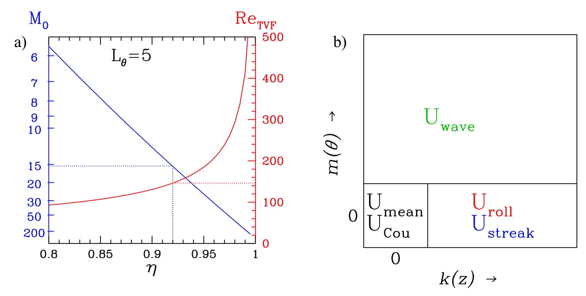
which diverges as the narrow-gap (or plane Couette) limit $\eta\rightarrow 1$ is approached [19]. The dependence of the critical Reynolds on $\eta$ is shown in Fig. 1(a), together with the relationship between $M_{0}$ and $\eta$ for $L_{\theta}=5$ . For $\eta=0.92$ , Taylor vortices appear above $Re_{\rm TVF}\approx 146$ . For these values of $\eta$ , $L_{z}$ , and $M_{0}$ , Taylor-vortex flow remains stable until $Re_{\rm WVF}\approx 201$ , above which the flow becomes unstable to wavy Taylor vortices. Figure 2(a) shows the Taylor-vortex flow while Fig. 3 shows the wavy-vortex flow, both computed at $Re=300$ .

Refer to caption — Figure 1: (a) Dependence of critical Reynolds number $Re^{\rm TVF}$ on the radius ratio $\eta$ for transition to Taylor-vortex flow (right scale). Also shown is the relationship between azimuthal wavenumber $M_{0}$ and $\eta$ for circumferential wavelength $L_{\theta}=5$ (left scale). Our chosen parameter values are $\eta=0.92$ and $M_{0}=15$ . (b) Schematic decomposition of flow into $\mathbf{U}_{\rm Cou}$ , $\mathbf{U}_{\rm mean}$ , $\mathbf{U}_{\rm roll}$ , $\mathbf{U}_{\rm streak}$ , $\mathbf{U}_{\rm wave}$ according to axial and azimuthal Fourier modes $k$ and $m$ .

III Analysis in terms of Self-Sustaining Process

We begin our analysis by introducing notation. Flow fields $\mathbf{U}$ can be decomposed as follows; see Fig. 1(b).


$\displaystyle\mathbf{U}$	$\displaystyle=$	$\displaystyle\sum_{k}\sum_{m}\left(\hat{U}^{k,m}_{r}(r)\mathbf{e}_{r}+\hat{U}^{k,m}_{\theta}(r)\mathbf{e}_{\theta}+\hat{U}^{k,m}_{z}(r)\mathbf{e}_{z}\right)e^{i(kz/L_{z}+mM_{0}\theta)}\qquad$	(6a)
	$\displaystyle=$	$\displaystyle\mathbf{U}_{\rm Cou}+\mathbf{U}_{\rm mean}+\mathbf{U}_{\rm roll}+\mathbf{U}_{\rm streak}+\mathbf{U}_{\rm wave}$	(6b)

where


$\displaystyle\mathbf{U}_{\rm Cou}$	$\displaystyle\equiv\left(Ar+\frac{B}{r}\right)\mathbf{e}_{\theta}$	(7a)
$\displaystyle\mathbf{U}_{\rm mean}$	$\displaystyle\equiv\hat{U}^{0,0}_{\theta}(r)\mathbf{e}_{\theta}-\mathbf{U}_{\rm Cou}$	(7b)
$\displaystyle\mathbf{U}_{\rm roll}$	$\displaystyle\equiv\sum_{k\neq 0}\left(\hat{U}_{r}^{k,0}(r)\mathbf{e}_{r}+\hat{U}_{z}^{k,0}(r)\mathbf{e}_{z}\right)\>e^{ikz/L_{z}}$	(7c)
$\displaystyle\mathbf{U}_{\rm streak}$	$\displaystyle\equiv\sum_{k\neq 0}\hat{U}_{\theta}^{k,0}(r)\mathbf{e}_{\theta}\>e^{ikz/L_{z}}$	(7d)
$\displaystyle\mathbf{U}_{\rm wave}$	$\displaystyle\equiv\sum_{k}\sum_{m\neq 0}\hat{\mathbf{U}}^{km}(r)e^{i(kz/L_{z}+mM_{0}\theta)}$	(7e)

Note that (7b) defines $\mathbf{U}_{\rm mean}$ to be the $(\theta,z)$ -independent deviation from laminar Couette flow $\mathbf{U}_{\rm Cou}$ , in contrast to Waleffe [22, 23, 24] whose mode ${\rm M}$ includes the laminar Couette solution (7a). In terms of this decomposition, Taylor-vortex flow and wavy-vortex flow take the form


$\displaystyle\mathbf{U}_{\rm TVF}$	$\displaystyle=\mathbf{U}_{\rm Cou}+\mathbf{U}_{\rm mean}+\mathbf{U}_{\rm roll}+\mathbf{U}_{\rm streak}$	(8a)
$\displaystyle\mathbf{U}_{\rm WVF}$	$\displaystyle=\mathbf{U}_{\rm Cou}+\mathbf{U}_{\rm mean}+\mathbf{U}_{\rm roll}+\mathbf{U}_{\rm streak}+\mathbf{U}_{\rm wave}$	(8b)

Waleffe’s Self-Sustaining Process [22, 23, 24] describes three steps involving the components $\mathbf{U}_{\rm roll}$ , $\mathbf{U}_{\rm streak}$ , and $\mathbf{U}_{\rm wave}$ :
A) $\mathbf{U}_{\rm roll}\Longrightarrow\mathbf{U}_{\rm streak}$ . This is a statement of kinematic advection of the azimuthal velocity.
B) $\mathbf{U}_{\rm streak}\Longrightarrow\mathbf{U}_{\rm wave}$ . This is described by Waleffe as a linear instability.
C) $\mathbf{U}_{\rm wave}\Longrightarrow\mathbf{U}_{\rm roll}$ . The nonlinear interaction of the wave with itself reinforces the rolls.

III.1 Rolls to streaks

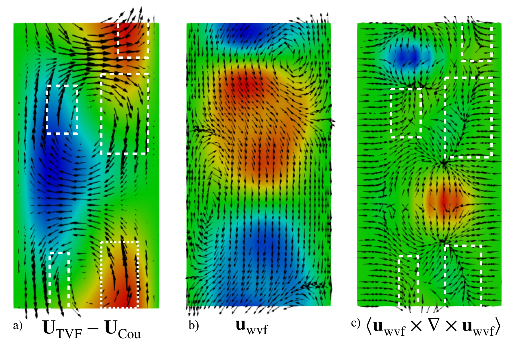
The SSP begins with streamwise invariant rolls $\mathbf{U}_{\rm roll}$ and considers the development of streaks from these rolls. Rolls transport fluid with high azimuthal velocity from the inner cylinder towards the outer cylinder and vice versa, causing the azimuthal velocity profile to vary along $z$ with the axial periodicity of the rolls. In plane Couette flow, or Waleffe’s free-slip version [24] now sometimes called Waleffe flow [28, 29, 30, 33, 34], rolls are not themselves an equilibrium state. Hence in the planar case it is necessary to initiate the SSP by inserting rolls into the flow and observing the resulting streak development. Permanent rolls and streaks have been produced in variants of plane Couette flow by including a spanwise-oriented wire or ribbon experimentally [35, 36, 37] or numerically [38]. For the Taylor-Couette problem, however, this phase is straightforward. The rolls and the streaks that they generate are contained in Taylor-vortex flow, which bifurcates supercritically and exists as a stable nonlinear equilibrium. In Fig. 2(a), calculated at $Re=300$ , the rolls are the meridional-plane flow indicated by arrows. The streaks are the axial variation in the azimuthal flow driven by the rolls and are seen as the colored patches.

III.2 Streaks to waves

We now turn to the second stage of the SSP in which the streaks become unstable to waviness. Once again, the situation in the Tayor-Couette problem is much more clear cut than in the planar case. The onset of waviness is a distinct supercritical instability – the transition from Taylor-vortex flow $\mathbf{U}_{\rm TVF}$ to wavy-vortex flow $\mathbf{U}_{\rm WVF}$ . In the $\mathbf{U}_{\rm WVF}$ state shown in Fig. 3, the flow has azimuthal variation (waviness) and is an azimuthally travelling wave. In 1985, Jones [10] suggested that the instability arose from the streaks, i.e. the axial variation of the azimuthal flow, which he called azimuthal jets. Thirty years later, Martinand, Serre and Lueptow [39] confirmed this idea by constructing the linear operator governing the wavy instability and showing that the eigenvalues of the portion of the operator arising from the azimuthal shear, i.e. the streaks, best matched the eigenvalues of the entire operator. They also demonstrated a number of common features between the transition to wavy vortex flow and the Kelvin-Helmholtz instability, notably a phase speed intermediate between that of the two cylinders and the multiplicity of possible azimuthal wavenumbers.

We show this by a different procedure, carrying out linearization about $\mathbf{U}_{\rm TVF}$ and about $\mathbf{U}_{\rm TVF}-\mathbf{U}_{\rm roll}$ , i.e. the Taylor vortex flow without its radial or axial components; see Eqs. (8). Fig. 4 compares the eigenvectors and growth rates resulting from these two linearizations. Since omitting $\mathbf{U}_{\rm roll}$ from the base flow barely changes the eigenvector or eigenvalue, it is clear that it plays no role in the instability. In contrast, linearization about $\mathbf{U}_{\rm TVF}-\mathbf{U}_{\rm streak}$ , i.e. omitting the axial dependence of the azimuthal flow, leads to eigenvalues with very small growth rate and eigenvectors with no resemblance to those of $\mathbf{U}_{\rm TVF}$ . (These results are not displayed.) These numerical experiments confirm that the instability mechanism responsible for the transition of $\mathbf{U}_{\rm TVF}$ to $\mathbf{U}_{\rm WVF}$ is the axial variation of the azimuthal velocity.

In addition to linearization, we examine the energy content in the flow components of the nonlinear states. We decompose both Taylor-vortex flow $\mathbf{U}_{\rm TVF}$ and the wavy-vortex flow $\mathbf{U}_{\rm WVF}$ into components given in Eqs. (6)-(8) and compute the energy of each. Fig. 5(a) shows the variation of the energy components as a function of Reynolds number. (The much larger energy of $\mathbf{U}_{\rm Cou}$ and a contribution combining ${\bf U}_{\rm Cou}$ and ${\bf U}_{\rm mean}$ are not shown.) $\mathbf{U}_{\rm TVF}$ appears at $Re=146$ and $\mathbf{U}_{\rm WVF}$ appears at $Re=201$ . It can be seen that ${\rm E}^{\rm WVF}_{\rm streak}$ , the energy of the streaks in ${\mathbf{U}}_{\rm WVF}$ , is substantially decreased from the analogous quantity ${\rm E}^{\rm TVF}_{\rm streak}$ in $\mathbf{U}_{\rm TVF}$ . This decrease is almost exactly counterbalanced by the energy in the waviness, ${\rm E}^{\rm WVF}_{\rm wave}$ , suggesting that the energy in the waviness is extracted from the streaks. The energy in the rolls is small and is almost the same in the two states. Thus, in addition to the linear instability mechanism, the comparison between the energy content of the saturated nonlinear states with and without waves shows that streaks feed the waves. As stated by Waleffe [24], it is not the rolls but the streaks whose energy is drained by the waves.

III.3 Waves to rolls

The key novelty of the SSP is the positive feedback of the waviness on the rolls. To study this in Taylor-Couette flow, we calculate the eigenvector $\mathbf{u}_{\rm wvf}$ responsible for the bifurcation to wavy vortices, shown in Fig. 2(b). (This complex eigenvector is shown here at one spatial or temporal phase.) We then compute the nonlinear interaction of $\mathbf{u}_{\rm wvf}$ with itself, in the form $\mathbf{u}_{\rm wvf}\times\nabla\times\mathbf{u}_{\rm wvf}$ . Since $\mathbf{u}_{\rm wvf}\sim e^{\pm iM_{0}\theta}$ , this quadratic term leads to azimuthal dependence of the form $e^{\pm 2iM_{0}\theta}$ (second harmonic) and $1$ (constant). We are interested in the constant contribution which has the form:

{\bf NL}\equiv\langle\mathbf{u}_{\rm wvf}\times\nabla\times\mathbf{u}_{\rm wvf}\rangle\equiv\mathbf{u}_{\rm wvf}^{R}\times\nabla\times\mathbf{u}_{\rm wvf}^{R}+\mathbf{u}_{\rm wvf}^{I}\times\nabla\times\mathbf{u}_{\rm wvf}^{I}

(9)

This term feeds back on the $\theta$ -independent contributions $\mathbf{U}_{\rm roll}$ , $\mathbf{U}_{\rm streak}$ and $\mathbf{U}_{\rm mean}$ . A visualization of this vector quantity is shown in Fig. 2(c). On a qualitative level, by comparing the arrows of Fig. 2(c) with those of Fig. 2(a), one can see the feedback of this term on $\mathbf{U}_{\rm roll}$ . The white-dashed boxes highlight regions in which the axial component of the Taylor-vortex flow is strong and aligned with the axial component of ${\bf\rm NL}$ . The resemblance is especially strong on near-axial curves in ${\bf NL}$ converging towards saddles above and below regions with high azimuthal component shown in red.

A more quantitative picture of the feedback is presented in Fig. 5(b). Shown is the normalized inner product between ${\rm NL}$ and each of $\mathbf{U}_{\rm roll}$ , $\mathbf{U}_{\rm streak}$ and $\mathbf{U}_{\rm mean}$ defined by:

\displaystyle\langle{\bf NL},{\bf U}_{---}\rangle

\displaystyle=\int_{0}^{L_{z}}dz\int_{r_{1}}^{r_{2}}r\>dr\>{\bf NL}(r,z)\cdot{\bf U}_{---}(r,z)

(10)

where ${\bf U}_{---}$ is any of $\mathbf{U}_{\rm roll}$ , $\mathbf{U}_{\rm streak}$ and $\mathbf{U}_{\rm mean}$ . It can be seen that ${\bf NL}$ has a positive overlap with ${\bf U}_{\rm roll}$ , meaning that indeed, the nonlinear interaction of $\mathbf{u}_{\rm wvf}$ with itself acts as a driving mechanism for rolls. ${\bf NL}$ also drives $\mathbf{U}_{\rm mean}$ . In contrast, ${\bf NL}$ has a negative overlap with ${\bf U}_{\rm streak}$ and hence this term tends to suppress the streaks.

IV Conclusion

According to the self-sustaining process (SSP) of [24], the building block of transition to turbulence in plane Couette flow and other wall-bounded shear flows, rolls induce streaks, which in turn undergo an instability to waviness, whose nonlinear interaction feeds the rolls. In plane Couette flow, laminar flow (the analogue of ${\bf U}_{\rm Cou}$ ) is stable for all Reynolds numbers; there is no equivalent of the steady Taylor-vortex flow. For Taylor-vortex flow, however, most of the steps of the SSP are already in place. Vortices (rolls) induce streaks (axially periodic variation of the azimuthal flow) kinematically via advection, as in plane Couette flow. We have confirmed that the instability to wavy-vortex flow is due to this variation [39]. In addition, we have shown that the energy of the waves in nonlinear wavy-vortex flow compensates almost exactly for the decreased energy in the streaks, as compared to the energy in the streaks of nonlinear Taylor-vortex flow. The third step is the feedback of the waves on the rolls, which is crucial for the SSP since in plane Couette flow the rolls do not arise from a linear instability leading to a nonlinear equilibrium. We have shown that this feedback mechanism exists in Taylor-Couette flow and that it is the rolls that are fed and not the streaks. The nonlinear self-interaction of the waves generates localized regions with strong axial forcing: this is the nature of the feedback on the Taylor vortices which closes the SSP.

Acknowledgements.

This research was partly supported by the grant TRANSFLOW, provided by the Agence Nationale de la Recherche (ANR).

References

[1] G.I. Taylor, “Stability of a viscous liquid contained between two rotating cylinders,” Phil. Trans. R. Soc. Lond. A 223, 289–343 (1923).
[2] Lord Rayleigh, “On the dynamics of revolving fluids,” Proc. R. Soc. Lond. A 93, 148–154 (1916).
[3] Donald Coles, “Transition in circular Couette flow,” J. Fluid Mech. 21, 385–425 (1965).
[4] Michael Gorman and Harry L Swinney, “Spatial and temporal characteristics of modulated waves in the circular Couette system,” J. Fluid Mech. 117, 123–142 (1982).
[5] Gregory P. King, Y. Li, W. Lee, Harry L. Swinney, and Philip S. Marcus, “Wave speeds in wavy Taylor-vortex flow,” J. Fluid Mech. 141, 365–390 (1984).
[6] C. David Andereck, S.S. Liu, and Harry L. Swinney, “Flow regimes in a circular Couette system with independently rotating cylinders,” J. Fluid Mech. 164, 155–183 (1986).
[7] J.J. Hegseth, G.W. Baxter, and C. David Andereck, “Bifurcations from Taylor vortices between corotating concentric cylinders,” Phys. Rev. E 53, 507 (1996).
[8] Steven T. Wereley and Richard M. Lueptow, “Spatio-temporal character of non-wavy and wavy Taylor-Couette flow,” J. Fluid Mech. 364, 59–80 (1998).
[9] C.A. Jones, “Nonlinear Taylor vortices and their stability,” J. Fluid Mech. 102, 249–261 (1981).
[10] C.A. Jones, “The transition to wavy Taylor vortices,” J. Fluid Mech. 157, 135–162 (1985).
[11] Philip S. Marcus, “Simulation of Taylor-Couette flow. part 1. numerical methods and comparison with experiment,” J. Fluid Mech. 146, 45–64 (1984a).
[12] Philip S. Marcus, “Simulation of Taylor-Couette flow. part 2. numerical results for wavy-vortex flow with one travelling wave,” J. Fluid Mech. 146, 65–113 (1984b).
[13] W.S. Edwards, S.R. Beane, and S. Varma, “Onset of wavy vortices in the finite-length Couette-Taylor problem,” Phys. Fluids 3, 1510–1518 (1991).
[14] J. Antonijoan and J. Sanchez, “On stable Taylor vortices above the transition to wavy vortices,” Phys. Fluids 14, 1661–1665 (2002).
[15] Masato Nagata, “Three-dimensional finite-amplitude solutions in plane Couette flow: bifurcation from infinity,” J. Fluid Mech. 217, 519–527 (1990).
[16] Hristina Hristova, Sébastien Roch, Peter J. Schmid, and Laurette S. Tuckerman, “Transient growth in Taylor-Couette flow,” Phys. Fluids 14, 3475–3484 (2002).
[17] Álvaro Meseguer, “Energy transient growth in the Taylor-Couette problem,” Phys. Fluids 14, 1655–1660 (2002).
[18] A. Prigent, G. Gregoire, H. Chate, O. Dauchot, and W. van Saarloos, “Large-scale finite-wavelength modulation within turbulent shear flows,” Phys. Rev. Lett. 89, 014501 (2002).
[19] Holger Faisst and Bruno Eckhardt, “Transition from the Couette-Taylor system to the plane Couette system,” Phys. Rev. E 61, 7227 (2000).
[20] Liang Shi, Marc Avila, and Björn Hof, “Scale invariance at the onset of turbulence in Couette flow,” Phys. Rev. Lett. 110, 204502 (2013).
[21] Grégoire Lemoult, Liang Shi, Kerstin Avila, Shreyas V. Jalikop, Marc Avila, and Björn Hof, “Directed percolation phase transition to sustained turbulence in Couette flow,” Nature Physics 12, 254–258 (2016).
[22] Fabian Waleffe, “Hydrodynamic stability and turbulence: Beyond transients to a self-sustaining process,” Stud. Appl. Math. 95, 319–343 (1995).
[23] James M. Hamilton, John Kim, and Fabian Waleffe, “Regeneration mechanisms of near-wall turbulence structures,” J. Fluid Mech. 287, 317–348 (1995).
[24] Fabian Waleffe, “On a self-sustaining process in shear flows,” Phys. Fluids 9, 883–900 (1997).
[25] Philip Hall and Frank T. Smith, “On strongly nonlinear vortex/wave interactions in boundary-layer transition,” J. Fluid Mech. 227, 641–666 (1991).
[26] Philip Hall and Spencer Sherwin, “Streamwise vortices in shear flows: harbingers of transition and the skeleton of coherent structures,” J. Fluid Mech. 661, 178–205 (2010).
[27] Hugh M Blackburn, Philip Hall, and Sherwin J Sherwin, “Lower branch equilibria in Couette flow: the emergence of canonical states for arbitrary shear flows,” J. Fluid Mech. 726, R2 (2013).
[28] Cédric Beaume, Edgar Knobloch, Gregory P. Chini, and Keith Julien, “Exact coherent structures in an asymptotically reduced description of parallel shear flows,” Fluid Dyn. Res. 47, 015504 (2014).
[29] Cédric Beaume, Gregory P. Chini, Keith Julien, and Edgar Knobloch, “Reduced description of exact coherent states in parallel shear flows,” Phys. Rev. E 91, 043010 (2015).
[30] Cédric Beaume, Edgar Knobloch, Gregory P. Chini, and Keith Julien, “Modulated patterns in a reduced model of a transitional shear flow,” Phys. Scr. 91, 024003 (2016).
[31] Thomas Duriez, Jean-Luc Aider, and José Eduardo Wesfreid, “Self-sustaining process through streak generation in a flat-plate boundary layer,” Phys. Rev. Lett. 103, 144502 (2009).
[32] Lukasz Klotz and José Eduardo Wesfreid, “Experiments on transient growth of turbulent spots,” J. Fluid Mech. 829, R4 (2017).
[33] Matthew Chantry, Laurette S. Tuckerman, and Dwight Barkley, “Turbulent–laminar patterns in shear flows without walls,” J. Fluid Mech. 791, R8 (2016).
[34] Matthew Chantry, Laurette S. Tuckerman, and Dwight Barkley, “Universal continuous transition to turbulence in a planar shear flow,” J. Fluid Mech. 824, R1 (2017).
[35] Olivier Dauchot and Francois Daviaud, “Finite amplitude perturbation and spots growth mechanism in plane Couette flow,” Phys. Fluids 7, 335–343 (1995).
[36] Sabine Bottin, Olivier Dauchot, and Francois Daviaud, “Intermittency in a locally forced plane Couette flow,” Phys. Rev. Lett. 79, 4377 (1997).
[37] Sabine Bottin, Olivier Dauchot, Francois Daviaud, and Paul Manneville, “Experimental evidence of streamwise vortices as finite amplitude solutions in transitional plane Couette flow,” Phys. Fluids 10, 2597–2607 (1998).
[38] Dwight Barkley and Laurette S. Tuckerman, “Stability analysis of perturbed plane Couette flow,” Phys. Fluids 11, 1187–1195 (1999).
[39] Denis Martinand, Eric Serre, and Richard M. Lueptow, “Mechanisms for the transition to waviness for Taylor vortices,” Phys. Fluids 26, 094102 (2014).