copyrightbox
Composite Hashing for Data Stream Sketches
Abstract
In rapid and massive data streams, it is often not possible to estimate the frequency of items with complete accuracy. To perform the operation in a reasonable amount of space and with sufficiently low latency, approximated methods are used. The most common ones are variations of the Count-Min sketch. By using multiple hash functions, they summarize massive streams in sub-linear space. In reality, data item ids or keys can be modular, e.g., a graph edge is represented by source and target node ids, a 32-bit IP address is composed of four 8-bit words, a web address consists of domain name, domain extension, path, and filename, among many others. In this paper, we investigate the modularity property of item keys, and develop more accurate, composite hashing strategies, such as employing multiple independent hash functions that hash different modules in a key and their combinations separately, instead of hashing the entire key directly into the sketch.
Our problem of finding the best hashing strategy is non-trivial, since there are exponential number of ways to combine the modules of a key before they can be hashed into the sketch. Moreover, given a fixed size allocated for the entire sketch, it is hard to find the optimal range of all hash functions that correspond to different modules and their combinations. We solve both problems with theoretical analysis, and perform thorough experiments with real-world datasets to demonstrate the accuracy and efficiency of our proposed method, MOD-Sketch.
I Introduction
In many domains such as real-time IP traffic, telephone calls, text data from email/SMS/blog/social media, web clicks and crawls, measurements from sensors and scientific experiments, rapid and massive volume of data are generated as a stream [10, 21]. In order to process fast streaming data, a growing number of applications relies on devices such as network interface cards, routers, switches, cell processors, FPGAs, and GPUs [25]; and usually these devices have very small on-chip memory. Whether in specialized hardware or in conventional architectures (e.g., static RAM, such as CPU cache), efficient processing of fast and large stream data requires creation of a succinct synopses in a single pass over that stream [8]. These summaries must be updated incrementally with incoming items. They should also support online query answering, e.g., estimating the frequency of an item in a long stream. Due to smaller summary sizes compared to the original stream, it is often not possible to answer queries with complete accuracy — reducing summary size increases the efficiency, but also reduces the accuracy.
We study frequency estimation queries over data streams: Given a data item as a query, we estimate the frequency count of that item in the input stream. In the literature, sketch data structures [11, 9, 3, 6, 16, 20] have been employed for frequency estimation queries. By using multiple hash functions, they summarize massive data streams within a limited memory space. For example in Figure 1(a), we depict the Count-Min sketch, having pairwise independent hash functions and each hash function with range . The key of every data item is hashed directly into the sketch.


In various settings, item keys are modular, i.e., consisting of multiple ordered parts. Many domains of stream data such as graph edges (e.g., web graphs, transportation networks, and social networks), IP addresses, telephone numbers, web addresses belong to this category. This enables us with more optimization scopes for hashing, such as one can hash different modules in a key and their combinations separately (i.e., composite hashing). In Figure 1(b), we illustrate an item key having modularity two, and the two parts are hashed via two independent hash functions separately, the first hash function with range and the second one with range . To allocate the same amount of space as Count-Min, we ensure that , and the sketch (referred to as the MOD-Sketch, an abbreviation for modular sketch) uses such pairs of hash functions. Two immediate questions that arise are as follows: (1) How does one select the optimal values of and ? (2) Between Count-Min and MOD-Sketch, which one results in more accuracy?
Our problems are non-trivial — answers to both questions depend on underlying properties of the stream and parameters of the sketch. For example, consider the case: ==, and a stream of graph edges in the form . Here, represents a directed edge from the source node to the target node , with frequency . Next, consider the edges having the same source node. MOD-Sketch maps the source node to same hash values, resulting in more collisions across edges having the same source node. This problem is exacerbated when the number of source nodes is more than that of target nodes in the graph stream. However, such skewness also allows us to find better MOD-Sketch parameters, e.g., . Similar optimization, on the contrary, is not possible for Count-Min. We find optimal values of and in a data-dependent manner: By sampling 11 1 Sampling a portion of the stream for estimating better sketch parameters has been considered earlier, e.g., in gSketch [32] and FCM [30]. It is worth noting that similar to those works, we assume that a sample of the original stream is available, which retains its important characteristics, e.g., distribution of high-frequency items. a small portion of the stream, and analyzing out-degrees of source nodes and in-degrees of target nodes in this sample. Furthermore, we decide the best choice between Count-Min and MOD-Sketch, again by sampling a small portion of the stream, and then based on the standard deviation of the values stored in different cells of these two sketches. We discuss our solutions with theoretical analyses, and demonstrate their performance with empirical results.
After studying the optimal hashing strategy for keys with modularity two, we focus on generalizations where keys can have higher modularity, e.g., a 32-bit IP address has modularity four (composed of four 8-bit words), thus opening the stage to a wider scope of optimizations. This problem is more complex due to two reasons. (1) There are exponential number of ways to combine the modules of a key before they can be hashed into the sketch. (2) Given a fixed , it is hard to find the optimal ranges of all hash functions that correspond to different modules and their combinations. We propose greedy heuristics, and empirically demonstrate that our method achieves higher accuracy compared to several baselines.
Our contribution and roadmap. We summarize our contributions below.
- •
We investigate the fundamental problem of constructing more accurate, composite hashing for sketches over data streams (§ III).
- •
We devise scalable, effective, and data-dependent solution for finding the optimal hashing ranges for different modules of an item key, with theoretical analyses (§ IV).
- •
We further generalize our algorithm to find good-quality hashing strategies for keys with modularity higher than two (§ V).
- •
We perform detailed experiments to demonstrate the accuracy, efficiency, and throughput of our developed MOD-sketch, comparing it with several baselines including Count-Min [9] and Equal-Sketch [19, 29], while also demonstrating its generalizability by implementing MOD-Sketch on top of the FCM sketch [30] (§ VI).
II Related Work
Data stream sketches. The problem of synopsis construction has been studied extensively [8] in the context of a variety of techniques such as sampling [15, 5] (including graph stream sampling, e.g., [24, 2]), wavelets [18, 14], histograms [17], sketches [11, 9, 3, 6, 16, 20], and counter-based methods, e.g., Space Saving [22] and Frequent [7]. Sketches and counter-based approaches are widely used for stream data summarization. Sketches are typically used for frequency estimation, which is the focus of this paper. Sketches keep approximate counts for all items, counter-based approaches maintain approximate counts only for the top- frequent items.
Among various sketches [9, 3, 6, 12, 13, 16, 20], Count-Min [9] is widely studied, it achieves good update throughput in general, as well as very high accuracy on skewed distributions. Several approaches have been proposed to further improve its accuracy, e.g., frequency-aware hashing (FCM [30], gSketch [32], and ASketch [26]), and non-uniform counter sizes (Cold Filter [34]). However, they do not consider the modularity of item keys unlike ours.
In the domain of graph edge stream, Count-Min has been extended to gMatrix [19] and TCM [29], which separately hash the source and target node ids corresponding to an edge. These approaches follow composite hashing. However, unlike ours, they allocate the same hashing range to both source and target nodes. Moreover, they do not address the problem of hashing data items with modularity higher than two. Composite hashing over IP data (i.e., having modularity four) is discussed in [28]. Once again, they allocate the same hashing range to all 4 bytes of the IP address. For generality, in this paper we refer to these prior works as Equal-Sketch. Based on detailed experiments, our proposed Mod-Sketch results in higher accuracy compared to Equal-Sketch.
Data-dependent and other composite hashing. Recently, data-driven learning methods for advanced hash functions (i.e., learning to hash) have become popular, particularly in the context of nearest neighbor queries (for a survey, see [31]). Composite hashing for nearest neighbor queries has been studied in [33]. While we select ranges of our composite hash functions in a data-dependent manner, our focus is sketches for data stream summarization. This is different from existing work on learning to hash for nearest neighbors.
III Preliminaries
The incoming data stream contains tuples , , , , . Here, denotes the arrival of the -th tuple with item having an associated positive count . In many applications, the value of is set to one, though we assume an arbitrary positive count in order to retain the generality of our model. As an example, in a telecommunication application, the frequency count may denote the number of seconds in the -th phone conversation. An item may appear multiple times in the stream, i.e., it is possible that , for . When we issue a query, e.g., finding the frequency of an item , we are looking for the aggregate count of that item in the stream so far. While sketch-based methods including ours can be adapted for time-window queries [1], as well as for removal of items [7] (i.e., a negative-count-update can be performed in the same way as a positive-count-update, so long as the overall count of an item never becomes negative), we do not consider them in this work. Furthermore, we use the notation interchangeably to denote an item as well as its key, because a key uniquely identifies an item.
An item key is often modular, that is, composed of ordered parts: . Here, denotes the generic representation of the -th module (i.e., co-ordinate) of a key. For an item key , we represent its modules as: Clearly, denotes the specific value in the -th module for item . As an example, in case of telecommunication network, each item is a communication (edge) from source to target users (nodes). The domains of source and target nodes are generally known apriori, and the edges between them arrive continuously in the stream. In case of modular keys, we assume that each module of a key can be from a predefined set of integers. This holds in reality, e.g., for a 32-bit IP address which consists four 8-bit words, each word can be from 000 to 255.
In this paper, we shall discuss our framework, MOD-Sketch (an abbreviation for modular sketch) as a composite hashing strategy on top of the Count-Min, one of the most widely-studied sketches. Nevertheless, the MOD-Sketch framework is generic, and it can be applied in combination with several other sketches. In our experiments in § VI-E, we also demonstrate the performance of MOD-Sketch when it is constructed with other underlying sketches. Next, for ease in the presentation, we introduce the standard Count-Min sketch.
III-A Count-Min
In Count-Min, a hashing approach is employed to approximately maintain the frequency counts of a large number of distinct items in a stream (Figure 1(a)). We use pairwise independent hash functions, each of which maps onto uniformly random integers in the range , where is the base of the natural logarithm, and are terms to define the error and the probabilistic error guarantee, respectively, which we shall introduce shortly. The data structure consists of a -dimensional array with cells of length and width . Each hash function corresponds to one of -dimensional arrays with cells each. Next, consider a data stream with items drawn from a massive set of domain values. When an item is received, we apply each of the hash functions to map onto a number in . The count of each of these cells is incremented by . To estimate the count of an item, we determine the set of cells to which each of the hash-functions maps, and compute the minimum value among all these cells. Let be the true value of the count being estimated. We note that the estimated count is at least equal to , since we are dealing with non-negative counts only, and there may be an over-estimation because of collisions in hash cells. It has been shown in [9] that for a data stream with arrivals, the estimate is at most with probability at least . In the event that the items have frequencies associated with them, we increment the corresponding count with the appropriate frequency. The same bounds hold in this case, except that we define as the sum of the frequencies of the items received so far.
For Count-Min to be effective, the hash functions are required to be pairwise independent. Following the Count-Min work [9], we select modular hash functions as follows.
| (1) |
Here, is a prime number larger than the maximum value of any key id , and is the range of the hash function. We select and uniformly at random from sets and , respectively.
III-B Hashing Keys with Modularity Two
We next introduce our problem for hashing keys with modularity two, i.e., . The hashing problem for higher modularity keys will be discussed in § V.
As we demonstrated in Figure 1, there are two possible choices for hashing the keys with modularity two. (1) Concatenate two ordered integer modules, construct a single integer id, i.e., , and hash it directly in the Count-Min. To distinguish between the keys such as and , we first consider the domains of the modules before concatenating them. For example, if the domain of each module is the set of integers , then is concatenated as , whereas is concatenated as . (2) Employ two independent hash functions that hash two modules of the key separately in MOD-Sketch. In total, MOD-Sketch uses such pairs of hash functions. All hash functions need to be pairwise independent, which is ensured by modular hash functions as in Equation 1. Let the range of the hash functions in Count-Min be , whereas for MOD-Sketch the ranges are and . To ensure the same amount of space, we have: . The other parameter, i.e., the number of hash functions, remains the same for both sketches, as the probability of the error bound is determined by , whereas the actual error bound depends on the range of the hash functions: , , .
Probabilistic accuracy guarantee. We now derive the accuracy guarantees for Count-Min and MOD-Sketch. It is important to note that one may not directly compare the error bounds of these two sketches, since the hashing strategies are different (i.e., Count-Min hashes concatenated keys, whereas MOD-Sketch performs composite hashing). In § IV-B, we shall introduce a more practical approach to select the best choice between them for a specific data stream.
Theorem 1.
Let the total frequency of items received so far in the stream be denoted by . Let be the true frequency of the item . Let be a very small fraction. Consider Count-Min with hash function range and width . Then, with probability at least , the estimated frequency is related to the true frequency by the following relationship:
| (2) |
The proof of Theorem 1 can be found in the Count-Min paper [9]. In Equation 2, the error term is relatively small if the true frequency is a significant fraction of the aggregate frequency . For real-world streams, which often has a skew [21], this holds for the high-frequency items.
Theorem 2.
Let the total frequency of items received so far in the stream be denoted by . Let be the true frequency of the item . Let be the sum of frequencies of the items having the first module as , and the sum of frequencies of the items having the second module as . Let be a very small fraction. Consider MOD-Sketch with hash function ranges and , as well as width . Then, with probability at least , the estimated frequency is related to the true frequency by the following relationship:
| (3) |
Proof.
Any incoming item, for which the ordered modules are neither nor , is equally likely to map onto one of cells of a hash function. The probability that any incoming item maps onto a particular cell is given by . Therefore, the expected number of spurious items for which the modules are neither nor , yet they get mapped onto the cell is given by . Let the number of such spurious items for the -th hash function be denoted by the random variable . Then, by the Markov inequality:
| (4) |
Next, we examine the case of spurious items for which the first module is . The number of such items is and the expected number of such items which map onto the entry is given by . Let be the random variable representing the number of such items. Then, by using the Markov inequality, we get:
| (5) |
Similarly, we denote by the random variable the number of items for which the second module is . The number of such items is and the expected number of such items which map onto the entry is given by . With Markov inequality, we have:
| (6) |
By combining the three above inequalities with the following rule , we get:
| (7) |
Taking the smallest estimate gives the best estimator, and the probability that this estimate violates the inequality in Equation 7 is the probability that all estimates exceed this error. The probability that this is true is given by at most . The result follows. ∎
For the above probability to be less than 1, we require . As earlier, since occurs in the exponent, the robustness of the above result can be magnified for modest values of .
III-C Problem Statement
We state our problems for hashing keys with modularity two as follows.
Problem 1.
For a data stream and a pre-defined length , find the most accurate MOD-Sketch range parameters and such that .
Problem 2.
For a data stream and a pre-defined length , select the most accurate sketch between Count-Min and MOD-Sketch having the same size, i.e., .
IV Algorithms for Modularity Two
IV-A Finding High-Quality MOD-Sketch Parameters
We set to find high-quality hashing ranges and for MOD-Sketch, by comparing its accuracy guarantee with that of a baseline technique. For the baseline method, we consider a special version of MOD-Sketch, referred to as the Equal-Sketch, where . Given a fixed and for a data stream, we select and such that the error of MOD-Sketch is as small as possible, compared to the error produced by Equal-Sketch. We note that the approach itself does not ensure finding optimal values of and . However, based on our empirical results, hashing ranges and found in this manner are of high-quality, and the accuracy of MOD-Sketch, in fact, becomes comparable to that of an exhaustive method which experimentally finds the best choice of hash function ranges corresponding to two modules of the key.
Theorem 3.
Consider an item with its estimated frequency via MOD-Sketch and Equal-Sketch as and , respectively. Let be the sum of frequencies of the items having the first module as , and the sum of frequencies of the items having the second module as . We denote by be the ratio: , and by the ratio: . Let be a very small fraction. Then, with a high probability, is smaller than by the largest margin when . Formally,
| (8) |
The difference of from is maximized when .
Proof.
We denote by the true frequency of the item . Let the total frequency of items received so far in the stream be . From Theorem 2, we get:
| (9) |
| (10) |
Given a pre-defined and a data item in the stream, Theorem 3 helps us to compute high-quality values of and for MOD-Sketch. For example, if we observe that is two times larger than , then we estimate as . Hence, compared to an Equal-Sketch with , the MOD-Sketch with and is expected to produce the least amount of error. Our result is intuitive, since suggests that there are generally large number of distinct source nodes than that of distinct target nodes, and this results in .
In Theorem 3, we compute a high-quality value of for a specific item in the stream. For a data stream, we assume that an apriori stream sample is available [32, 30], which retains important characteristics of the original stream, e.g., distribution of high-frequency items. For every item present in the sample, we estimate its related from the sample. Next, we employ an aggregate operator (e.g., minimum, maximum, median, average, etc.) to compute the aggregated . We finally derive as . We illustrate our method with an example below. Based on our detailed empirical evaluation over several real-world stream datasets, we find that about 24% initial stream sample, together with the median aggregate of , is generally sufficient to estimate a high-quality value of .
Example 1.
Assume from the initial stream sample, we obtained items: with aggregated frequency , respectively. We compute values for these items: . Analogously, we find , . We compute the median of these values, i.e., median of the multi-set consisting of for times, for times, and for times. Thus, .
IV-B Choice between MOD-Sketch & Count-Min
We next consider Problem 2: For a data stream and a pre-defined length , select the most accurate sketch between Count-Min and the optimal MOD-Sketch having the same size, i.e., . Unlike Theorem 3, we may not directly compare the error bounds of these two sketches, since the hashing strategies are different. We design a more practical approach by computing the standard deviation of the count values stored in different cells of these sketches. Theorem 13 states that the sketch with the smaller standard deviation generally results in less error for the frequency estimation.
Theorem 4.
Consider two sketches and having the same size: , such that the standard deviations of count values stored in different cells of these sketches are and , respectively. Assume . Let us consider an item with its estimated frequency via and as and , respectively. Assume . Then, with probability at least , the following holds:
| (13) |
Proof.
Let the total frequency of items received so far in the stream be . Let the values stored in the cells of be denoted by the random variable . The expected value of is , which is the mean value of the counts in the sketch. By using the Cantelli’s inequality, with , the possibility of the lower bound of can be measured as follows.
| (14) |
Analogously, let the values stored in the cells of be denoted by the random variable . The expected value of is . By employing the Cantelli’s inequality, we have:
| (15) |
The above inequality can be written as follows.
| (16) |
Combining two inequalities in Equations 14 and 16, we get:
| (17) |
This completes the proof. ∎
Hence, by comparing the variance of two sketches with the same and (but with different hashing techniques), one can predict which sketch would result in less frequency estimation error for the given data stream. In practice, we consider an initial sample of the incoming stream, and store it in the two sketches having same . Then, based on the standard deviation of the values stored in different cells of these sketches, we decide which sketch we shall use.
V Algorithms for Modularity Two
In this section, we consider the generalization of our problem for item keys with modularity higher than two. Two natural baselines for hashing such keys are: (1) Count-Min, i.e., concatenate ordered modules of the key and hash it directly with a hash function of range , and (2) Equal-Sketch, i.e., separately hash modules with independent hash functions, each having equal range . However, a more accurate MOD-Sketch could combine some modules of the key and hash them together, and could separately hash the remaining modules. Therefore, it raises the problem of how to design a more accurate MOD-Sketch for a given key with modularity higher than two, considering modules might be combined or kept separate as necessary.
V-A An Exact Strategy
Let us consider keys of modularity , i.e., . There are exponentially large number of ways to combine the modules — also known as the “Bell number”, which counts the possible partitions of a set. We denote by the total number of ways one can combine different parts of a key having modularity . Then, we have:
| (18) |
with base cases: . .
| 2 | 5 | 15 | 52 | 203 | 877 | 4140 | 21147 | 115975 | |
| 4 | 8 | 16 | 32 | 64 | 128 | 256 | 512 | 1024 |

Proof.
We shall assume that , since the base cases for and are already given. Let us consider the first module in order, i.e., . Clearly, the number of ways remains as a separate module is . Next, we consider the number of ways can be combined with exactly one of the remaining modules. The number of remaining modules is , and after is combined with exactly one of the remaining modules, e.g., , we have total possible ways. In general, when is combined with exactly of the remaining modules, where , total number of possible ways is . By combining all these counts as they are mutually exclusive, the result follows. ∎
Notice that for , (Table I). We observe that , in fact, increases at a much higher rate than . Therefore, an exact method to verify all possible ways of combining the modules and thereby finding the best option would be extremely time consuming. In this paper, we keep open the complexity of finding an exact solution for our problem having modularity greater than two. Instead, we develop a more scalable, greedy approach.
V-B Greedy Solution
We discuss our algorithm in two phases.
V-B1 Range Ratio Computation
Our first problem is: Given a total length and a specific way of combining the modules, how shall we find the optimal range of all hash functions that correspond to different (combined) parts of the key? In particular, consider modules: , and a specific way of combining them, i.e., , where each is a singleton, or a combination of some modules that are hashed together. For , and do not have a common module. Moreover, and are separately hashed for all . Clearly, , and each key is hashed using independent hash functions. Given a length parameter , we aim at finding the optimal ranges of these hash functions, where .


Recall that for keys having modularity two, we developed our solution in § IV-A. We now generalize our method for keys with modularity more than two with a recursive strategy as follows. We start by measuring the range ratio between (corresponding to the last hash function) and the rest. Formally, we take the parts as a combined part, then we calculate the ratio of ranges , where . We compute with our method in § IV-A, that is, . We measure , .
Next, we recursively calculate the ratio where . We repeat this process until we find the ratio .
Our recursive steps are illustrated in Figure 2. The time complexity to compute the optimal values of by our method is , where , being the number of modules. We next discuss the details of the greedy approach.
V-B2 Greedy Algorithm
Our greedy algorithm works by traversing the search space in a depth-first manner until a path of length has been found covering all the modules. In Figure 3, we demonstrate our method with keys of modularity : . We start with the first module in order, which is , and verify four possibilities, that is, hashing separately (denoted by the dotted arrow between and ), or combining with one of the remaining modules, , , or (denoted by solid arrows between these nodes). Among these four possibilities, we greedily find the best strategy, e.g., in Figure 3 we already selected the best strategy as to hash separately.
By traversing the dotted edge from to , we arrive at the current module . At this intermediate stage, we have three choices: Hashing separately (denoted by the dotted arrow between and ), or combining with one of the remaining modules, or (denoted by solid arrows between these nodes). Again, we greedily find the best strategy, e.g., in Figure 3 we already selected the best strategy as to combine and .
In particular, at any intermediate stage (), we have computed the configuration with modules, and next we have to select from choices in a greedy manner. For example in Figure 3, we decided the configuration among three modules , , , i.e., to keep separate and to combine , . Now, we have two choices: Further combine with , or keep them separate. We make a greedy selection between these two choices, and finally terminate our method.
Our complete procedure is given in Algorithm 1. Note that by greedy selection, we only consider choices for combining the modules, as opposed to the exact number of ways in which the modules can be combined. We have shown in Table I that increases at a higher rate compared to , and this demonstrates the scalability of our algorithm. Moreover, at any intermediate stage , since we do not change the optimal configuration with modules obtained previously, some of the optimal range ratio estimations from earlier stages could be re-used. For example, assume in Figure 3, out of two hashing options, the best one selected is to separate and . Thus, the three separate parts of the key are , , and . To find the optimal hashing ranges due to these three parts by following our recursive method in Section V-B1, one needs to compute the range ratio of the parts and . However, this ratio has been already computed in Figure 3, and therefore, can be re-used. Such re-using of range ratio estimation further improves our efficiency.
VI Experimental Results
VI-A Environment Setup
VI-A1 Datasets
We consider six real-world stream datasets from two sources. (1) Twitter Communication Stream: We obtain the Twitter graph dataset from https://snap. stanford.edu/, which consists of all public tweets during a 7-month period from June 1, 2009 to December 31, 2009. Each edge (directed) in our dataset represents a communication between two users in the form of a re-tweet. The edge frequency is defined as the number of communications between the corresponding source and target users. Clearly, every item (i.e., an edge) in this dataset has modularity two, consisting of a source and a target node. (2) IPv4 Trace Stream: We use two IP trace streams from the IPv4 Routed /24 Topology dataset (http://www.caida.org/data/overview/), which contains the raw IPv4 team-probing data from January 1, 2008 to December 31, 2008 by CAIDA. We obtain two datasets of IP address streams from source-to-destination and source-to-respond traces, and refer to them as IPv4-1 and IPv4-2, respectively. Each item in both datasets contains two 4-bytes IP addresses. Therefore, both IPv4-1 and IPv4-2 have modularity eight, denoted as IPv4-1#8 and IPv4-2#8. Next, we generate modularity-two datasets from IPv4-1#8 and IPv4-2#8 by hashing each IP address to one integer id, thereby obtaining datasets IPv4-1#2 and IPv4-2#2. Similarly, we generate modularity-four datasets by hashing each IP address with two integer ids — the first integer corresponds to the first 2-bytes of the IP address, and the second one corresponds to the next 2-bytes of the IP address. In this way, we obtain another two datasets IPv4-1#4 and IPv4-2#4, having modularity four.
In Table II, the flat stream size represents the total stream size that contains repetition of items. The compressed stream size, in contrast, is defined as the size of all distinct items that have nonzero frequency, along with their frequency counts. Both flat stream and compressed stream can answer our queries with complete accuracy. We shall demonstrate in our experiments that MOD-Sketch, though a small fraction of the flat and compressed stream representations, achieves reasonably high accuracy.
In Table III, we show additional statistics for our three datasets with modularity two.
| Datasets | Modul | # Distinct | Agg. item | Max. item | Flat | Compressed |
| -arity | items | frequency | frequency | stream | stream | |
| (GB) | (GB) | |||||
| 2 | 78 508 963 | 151 | 17 149 | 3.69 | 0.15 | |
| IP-1 | 2 | 94 820 182 | 6 204 | 123 614 | 7.23 | 1.72 |
| IP-1 | 4 | 94 820 182 | 6 204 | 123 614 | 9.50 | 2.26 |
| IP-1 | 8 | 94 820 182 | 6 204 | 123 614 | 13.42 | 4.19 |
| IP-2 | 2 | 94 890 903 | 6 562 | 106 956 | 17.98 | 1.81 |
| IP-2 | 4 | 94 890 903 | 6 562 | 106 956 | 22.79 | 3.29 |
| IP-2 | 8 | 94 890 903 | 6 562 | 106 956 | 30.35 | 5.05 |
| Datasets | #Source nodes | #Target nodes |
|---|---|---|
| 4 790 726 | 15 062 341 | |
| IP-12 | 7 234 121 | 665 279 |
| IP-22 | 8 352 656 | 697 121 |
VI-A2 Comparing methods
We compare MOD-Sketch with three following methods. (1) Count-Min [9], i.e., concatenate ordered modules of the key and hash it directly with a hash function of range . We use such pairwise independent hash functions. (2) Equal-Sketch, i.e., separately hash modules with independent hash functions, each having range . We use such pairs of hash functions. In the context of graph edge stream (i.e., having modularity two), similar methods were explored, e.g., TCM [29] and gMatrix [19]. (3) Exhaustive, i.e., empirically evaluate all possibilities of combining the modules of a key (the exact value of can be obtained from Table I). For each possibility, experimentally find the best choice of hash function ranges corresponding to different (combined) parts of the key. Finally, select the best option that minimizes the frequency estimation error. Clearly, the Exhaustive approach is very expensive, and it does not scale well beyond modularity .
VI-A3 System description
We implement our code in Python, and perform experiments on a single core of 2.40GHz Xeon server. Each experiment uses less than 1GB of the main memory, and our empirical results are averaged over 10 runs.


VI-A4 Evaluation metrics
We present the accuracy of frequency estimation queries using observed error [9], which is measured as the difference between the estimated frequency and the true frequency, accumulated over all the items queried. The observed error is expressed as a ratio over the aggregate true frequency of all the items queried.
We generate two types of query sets: (1) Top- query consists of the top- high frequency items. (2) Random- query consists of randomly selected items from the data stream.
VI-B Results for Modularity Two
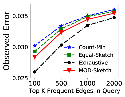
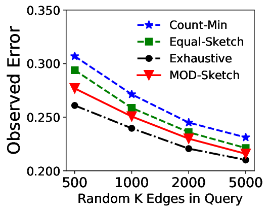
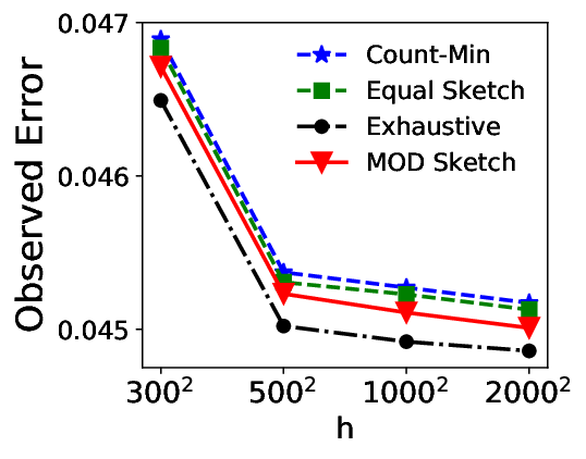
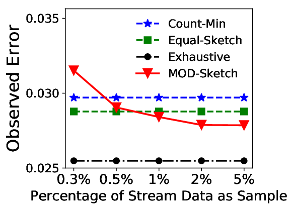
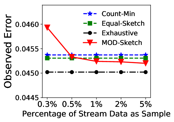
In Figures 4 and 5, we show the accuracy of edge frequency queries over our datasets with modularity two, under varying of both top- and random- queries, and for different range parameter . We notice that in all experiments, MOD-Sketch obtains smaller observed error compared to Count-Min and Equal-Sketch. As an example, in Twitter, MOD-Sketch with and has a relatively lower observed error, compared to Count-Min of one combined range and Equal-Sketch of two equal ranges . Compared to Exhaustive, which empirically finds the optimal parameters: and , the setting of MOD-Sketch is very similar. Further delving into the Twitter dataset, we find that the distinct number of target nodes is more than that of source nodes. This justifies why our method MOD-Sketch, as well as Exhaustive report in the optimal setting. We find similar observations with IPv4-1 and IPv4-2.
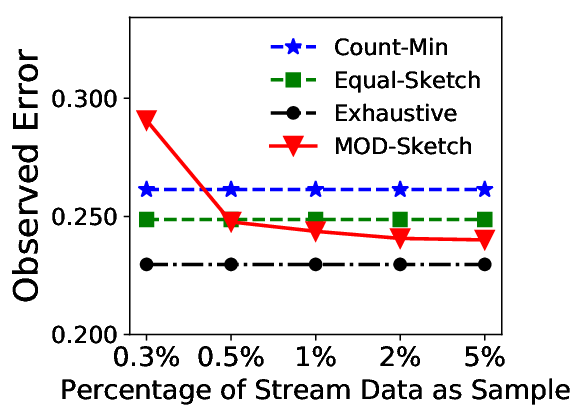
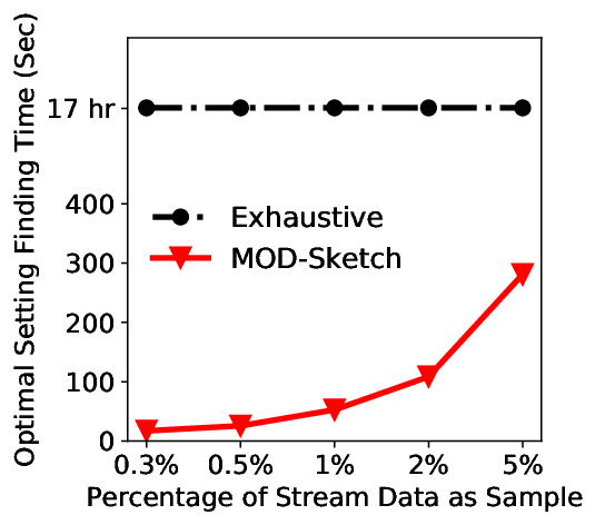
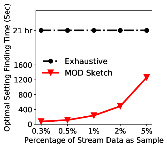
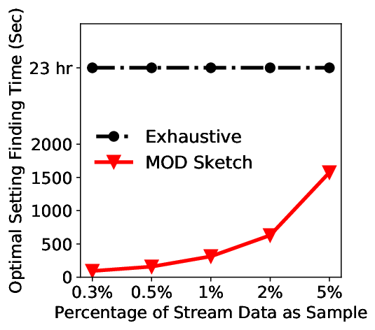
While Exhaustive produces the least observed error, finding the optimal parameters experimentally by considering various combinations requires about 20 hours, which is not affordable (Figure 6). In comparison, MOD-Sketch requires a few minutes (520 minutes) to find good-quality and values that result in comparable accuracy with Exhaustive. Moreover, the observed error of MOD-Sketch reduces when the size of the data sample for its parameter estimation increases. We find that with about 2% of the stream, the observed error converges (Figure 5), therefore in our experiments, we use 2% of the stream for parameter estimation.
VI-C Results for Modularity Two
We analyze the accuracy of edge frequency estimation over our datasets with modularity 4 and 8, and with varying (Figure 7). The observed error increases with higher modularity. However, the observed error of MOD-Sketch is always smaller than that of Equal-Sketch and Count-Min, and is also comparable to Exhaustive. In fact, for modularity 8, the observed error of MOD-Sketch is almost half of that due to Count-Min and Equal-Sketch.
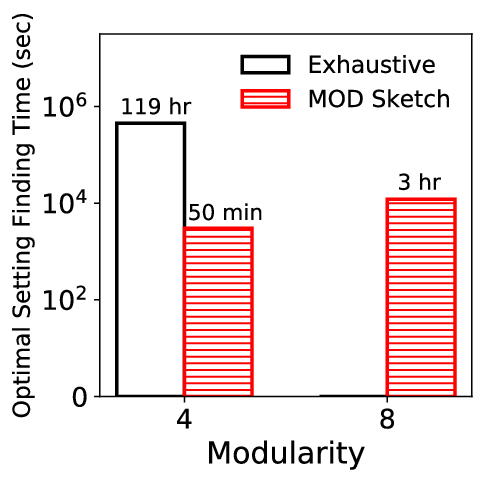
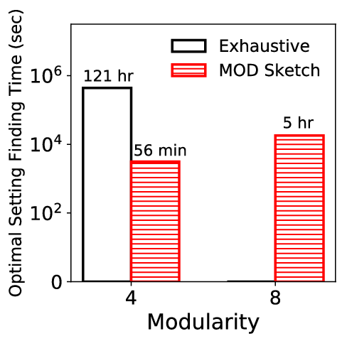
Moreover, the running time to find the optimal parameters using Exhaustive is at least two orders of magnitude higher than that of MOD-Sketch for modularity 4. In fact, with modularity 8, Exhaustive does not complete within 100 hours (Figure 9). These results demonstrate the efficiency and scalability of MOD-Sketch over highly-modular data streams.
VI-D Stream Processing Throughput
The throughputs of MOD-Sketch, Count-Min, and Equal-Sketch are close when the modularity is small (Figure 8). For streams with higher modularity, the throughput of MOD-Sketch is lower than that of Count-Min, but higher than that of Equal-Sketch. This can be explained as follows. For an item with modularity , Count-Min uses hash functions, whereas Equal-Sketch employs hash functions. Since MOD-Sketch optimally combines some modules of the key, the number of hash functions used by it is less than , but more than . In all our experiments, the throughput of MOD-Sketch varies between 30K90K items second.
VI-E Generalizability
We evaluate the generalizability of MOD-Sketch by implementing it on top of the FCM sketch [30]. FCM improves the accuracy of Count-Min by employing different number of hash functions for high-frequency and low-frequency items, detected by an additional Misra-Gries counter [23]. FCM first applies two separate hash functions to compute an offset and a gap, which determines the subset of hash functions to be used for hashing the item. Then, it utilizes the selected hash functions to hash the item into the sketch. We refer to our implementation of MOD-Sketch on top of FCM as FMOD (Figure 10). As expected, FCM reduces the observed error compared to Count-Min. However, our designed FMOD further reduces the observed error even compared to FCM. These results demonstrate the generalizability of MOD-Sketch.
VI-F Effectiveness of Median Aggregate
In Figure 11, we demonstrate the effectiveness of our median aggregate for selecting the parameter , compared to other aggregates: minimum, maximum, and average. The median aggregate produces less observed error, this is because the estimations from maximum and average (minimum) are greatly affected by a few sampled items with extremely large (small) frequency in a skewed distribution. In contrast, the median estimate avoids such issues.
VII Conclusions


We present MOD-Sketch to improve the accuracy of sketches by employing multiple independent hash functions that hash different modules in a key and their combinations separately. We develop scalable algorithms that sample a small portion of the stream, and find the optimal strategy to combine different modules of the key before they are hashed into the sketch. Furthermore, we compute good-quality hashing ranges for various combined parts of the key. Based on our empirical results over six real-world data streams, MOD-Sketch outperforms several baselines including Count-Min, and it can be used together with more sophisticated sketches, e.g., FCM to further improve the frequency estimation accuracy. In future work, it would be interesting to consider how to update MOD-Sketch parameters when the distribution of the items in the stream change over time.
References
- [1] C. Aggarwal, J. Han, J. Wang, and P. Yu, “A Framework for Clustering Evolving Data Streams”, VLDB, 2003.
- [2] N. K. Ahmed, N. Duffield, T. L. Willke, and R. A. Rossi, “On Sampling from Massive Graph Streams”, PVLDB, vol. 10, no. 11, pp. 1430–1441, 2017.
- [3] N. Alon, Y. Matias, and M. Szegedy, “The Space Complexity of Approximating the Frequency Moments”, STOC, 1996.
- [4] B. H. Bloom, “Space/time Trade-offs in Hash Coding with Allowable Errors”, Comm. of ACM, vol. 13, issue 7, pp. 422–426, 1970.
- [5] E. Cohen, “Stream Sampling for Frequency Cap Statistics”, KDD, 2015.
- [6] M. Charikar, K. Chen, and M. Farach-Colton, “Finding Frequent Items in Data Streams”, ICALP, 2002.
- [7] G. Cormode and M. Hadjieleftheriou, “Finding Frequent Items in Data Streams”, PVLDB, vol. 1, no. 2, pp. 1530–1541, 2008.
- [8] G. Cormode and M. Garofalakis and P. J. Haas and C. Jermaine, “Synopses for Massive Data: Samples, Histograms, Wavelets, Sketches”, Foundations and Trends in Databases, vol. 4, no. 1–3, pp. 1–294, 2012.
- [9] G. Cormode and S. Muthukrishnan, “An Improved Data-Stream Summary: The Count-min Sketch and its Applications”, J. of Algorithms, vol. 55, no. 1, 2005.
- [10] G. Cormode, T. Johnson, F. Korn, S. Muthukrishnan, O. Spatscheck, and D. Srivastava, “Holistic UDAFs at Streaming Speeds”, SIGMOD, 2004.
- [11] A. Dobra, M. Garofalakis, J. Gehrke, and R. Rastogi, “Processing Complex Aggregate Queries over Data Streams”, SIGMOD, 2002.
- [12] C. Estan and G. Varghese, “New Directions in Traffic Measurement and Accounting: Focusing on the Elephants, Ignoring the Mice”, ACM Trans. Comput. Syst., vol. 21, no. 3, pp. 270–313, 2003.
- [13] M. Fang, N. Shivakumar, H. Garcia-Molina, R. Motwani, and J. Ullman, “Computing Iceberg Queries Efficiently”, VLDB, 1998.
- [14] M. Garofalakis and P. B. Gibbons, “Wavelet Synopses with Error Guarantees”, SIGMOD, 2002.
- [15] S. Ganguly, P. B. Gibbons, Y. Matias, and A. Silberschatz, “Bifocal Sampling for Skew-Resistant Join Size Estimation”, SIGMOD, 1996.
- [16] A. C. Gilbert, Y. Kotidis, S. Muthukrishnan, and M. Strauss, “How to Summarize the Universe: Dynamic Maintenance of Quantiles”, VLDB, 2002.
- [17] S. Guha, N. Koudas, and K. Shim, “Data-streams and Histograms”, STOC, 2001.
- [18] A. C. Gilbert, Y. Kotidis, S. Muthukrishnan, and M. Strauss, “Surfing Wavelets on Streams: One-Pass Summaries for Approximate Aggregate Queries”, VLDB, 2001.
- [19] A. Khan and C. Aggarwal, “Toward Query-Friendly Compression of Rapid Graph Streams”, Social Netw. Analys. Mining, vol. 7, no. 1, pp. 23:1–23:19, 2017.
- [20] B. Krishnamurthy, S. Sen, Y. Zhang, and Y. Chen, “Sketch-based Change Detection: Methods, Evaluation, and Applications”, IMC, 2003.
- [21] N. Manerikar and T. Palpanas, “Frequent Items in Streaming Data: An Experimental Evaluation of the State-of-the-art”, Data Knowl. Eng., vol. 68, no. 4, pp. 415–430, 2009.
- [22] A. Metwally, D. Agrawal, and A. E. Abbadi, “Efficient Computation of Frequent and Top-k Elements in Data Streams”, ICDT, 2005.
- [23] J. Misra and D. Gries, “Finding Repeated Elements”, Science of Computer Programming, vol. 2, no. 2, pp. 143–152, 1982.
- [24] A. Pavan, K. Tangwongsan, S. Tirthapura, and K.-L. Wu, “Counting and Sampling Triangles from a Graph Stream”, PVLDB, vol. 6, no. 14, pp. 1870–1881, 2013.
- [25] O. Rottenstreich, Y. Kanizo, and I. Keslassy, “The Variable-Increment Counting Bloom Filter”, IEEE/ACM Trans. Netw., vol. 22, no. 4, pp. 1092–1105, 2014.
- [26] P. Roy, A. Khan, and G. Alonso, “Augmented Sketch: Faster and More Accurate Stream Processing”, SIGMOD, 2016.
- [27] F. Rusu and A. Dobra, “Sketches for Size of Join Estimation”, ACM TODS, vol. 33, no. 3, pp. 15, 2008.
- [28] R. Schweller, Z. Li, Y. Chen, Y. Gao, A. Gupta, Y. Zhang, P. A. Dinda, M.-Y. Kao, and G. Memik, “Reversible Sketches: Enabling Monitoring and Analysis over High-speed Data Streams”, IEEE/ACM Trans. Netw., vol. 15, no. 5, pp. 1059–1072, 2007.
- [29] N. Tang, Q. Chen, and P. Mitra, “Graph Stream Summarization: From Big Bang to Big Crunch”, SIGMOD, 2016.
- [30] D. Thomas, R. Bordawekar, C. Aggarwal, and P. S. Yu, “On Efficient Query Processing of Stream Counts on the Cell Processor”, ICDE, 2009.
- [31] J. Wang, W. Liu, S. Kumar, S.-F. Chang, “Learning to Hash for Indexing Big Data - A Survey”, Proceedings of the IEEE, vol. 104, no. 1, pp. 34–57, 2016.
- [32] P. Zhao, C. Aggarwal, and M. Wang, “gSketch: On Query Estimation in Graph Streams”, PVLDB, vol. 5, no. 3, pp. 193–204, 2011.
- [33] D. Zhang, F. Wang, L. Si, “Composite Hashing with Multiple Information Sources”, SIGIR, 2011.
- [34] Y. Zhou, T. Yang, J. Jiang, B. Cui, M. Yu, X. Li, and S. Uhlig, “Cold Filter: A Meta-Framework for Faster and More Accurate Stream Processing”, SIGMOD, 2018.