Use Of Vapnik-Chervonenkis Dimension in Model Selection
by
Merlin T. Mpoudeu
A DISSERTATION
Presented to the Faculty of
The Graduate College at the University of Nebraska
In Partial Fulfillment of Requirements
For the Degree of Doctor of Philosophy
Major: Statistics
Under the Supervision of Professor Bertrand Clarke
Lincoln, Nebraska
August, 2017
Use Of Vapnik-Chervonenkis Dimension in Model Selection
Merlin T. Mpoudeu, Ph.D.
University of Nebraska, 2017
Acknowledgements
I would especially like to thank my advisor Bertrand Clarke. Without his insight, encouragement, probing questions, excitement, and suggestions, this thesis would have ended up much differently. I am very proud of this work, and I owe him a tremendous amount for helping it to become something valuable. I would also like to thank Professor Kent M. Eskridge for the help that he provided through his Friday consulting group.
I would like to thank Dr. Jennifer Clarke, Dr. Yumou Qiu and Dr Stephen Scott for being my graduate committee members and reviewing my dissertation. Their help and suggestions have been invaluable on both academic and personal levels.
I am grateful to my friends (Cyrile Nzouda, Salfo Bikienda, and Kismiantini); you have been with me since the beginning, and your support through the last four years has been invaluable.
I would like to express my gratitude to my parents, Mbialeu Charles and Siewe Philomene, and my brother and sisters for their encouragement throughout this graduate school process. I would also like to thank two and most import people in my life: My fiancee Anne Mbenya and my 20 month old son Charles Mpoudeu for their support and patience.
INTRODUCTION
Given a dataset of size , there are different dichotomies of the observations. If we have a collection of functions so that given any dichotomy of the dataset, there is a function that is consistent with the dichotomy then we say that generates the datasets. The Vapnik-Chervonenkis Dimension (VCD) is the maximum value of data points all whose dichotomies can be generated by . This measures the richness of .
The earliest usage of what we now call the VCD seems to be in Vapnik and Chervonenkis (1968). A translation into English was published as Vapnik and Chervonenkis (1971). The VCD was initially called an index of a collection of sets with respect to a sample and was developed to provide sufficient conditions for the uniform convergence of empirical distributions. It was extended to provide a sense of dimension for function spaces, particularly for functions that represented classifiers. After two decades of development this formed the foundation for the field of Statistical Learning Theory, summarized in Vapnik (1999) and extensively treated in Vapnik (1998). An intuitive treatment of VCD from the classification perspective can be found in Moore (2001). Aside from the development in statistical learning, VCD plays an important role in various real analysis settings. For instance, VCD defines VC classes of functions that have relatively small covering numbers, see Pollard (1984), Devroye (1996), Van der Waart (1998), and van de Geer (2000) amongst others. At the risk of oversimplification, the VCD of a space of functions is currently seen mostly as a parameter characterizing bounds of cumulative risks in term of the size of the function class.
One of our goals is to estimate the true value of the VCD (noted ) of a data generator (DG) by, say, and use as the estimated complexity of the model class; e.g, linear models. Given , the next step is to perform model selection. In fact, we use the notion of ‘consistency at the true model’ to do so. We define ‘consistency at the true model’ to be
- 1.
consistency at the true model in the usual sense of the term, basically we expect that in probability as the sample size increases, coupled with
- 2.
some kind of identifiable bad behaviour away from the true model, getting worse as the wrong model moves further from the true model.
If we have a list of non-nested models with nested VCD’s denoted by , and we would like to perform model selection, we can estimate by setting
| (1) |
where is some set of models and is calculated using model . Writing , we see that is a function of the VCD of the conjectured model and in (1) removes this dependence. In the special case that ’s are linear i.e. , we will see that (here, ). In practice we an approximate form of (1) by thresholding the difference within the ; see (3.6) in Subsec. 3.4.2.
We can also order the inclusion of the covariates using a shrinkage method such as SCAD (see Fan and Li (2001)) or the correlation (see Fan and Lv (2008)) and the use to pick a model. We also upper bounded the true but unknown risk by an expression that depends on . We used that expression for model selection. In fact, for each model on the list, we estimate a VCD for it and use the estimate in an upper bound of the unknown risk. Then we pick the model with the smallest upper bound on its risk. Asymptotically, the chosen model should perform well with higher probability. This technique is called Empirical Risk Minimization and is suitable for non-nested model lists.
While VCD is not in general equivalent to the real dimension, in the special case of linear models VCD and the real dimension are the same. Thus, at a minimum, with linear models, we can cut down the plausible models to those that have at least parameters – and hopefully not too many more.
The estimation of is done in three steps: first we find the Expected Maximum Difference Between Two Empirical Losses (EMDBTEL). This value depends on the model class (the class of linear models for this case), the design points, the number of bootstrap samples we draw from our data, and the number of intervals used to discretrize the loss function. In fact, if the number of the design points is , we will have different values of the EMDBTEL. Since, the bound on the EMDBTEL is not tight, the next step is to find the best factor on the RHS of (2.21) i.e. the value of that will minimize the upper bound. The final step is the estimation of . This is done by minimizing the squared distance between the EMDBTEL (the LHS of (2.21)) and the upper bound (the RHS of (2.21)). The intuition is that this minimum corresponds to the decision problem, or more precisely the model class, that has the fastest convergence to zero of its expected supremal difference of cumulative empirical losses and hence would be the ‘right’ problem for us to solve if only we knew it. Therefore, even though the model class is only implicitly defined, we can take its or empirically, , as a lower bound on the VCD of model classes. in the examples presented here our objective function has a unique minimum that can be taken as an estimate of . In practice, for finite sample sizes this is best regarded as a lower bound on . Indeed, in practice, we can estimate several values of , take their average and standard deviation as a way to get what is effectively a bootstrap confidence interval for .
Our contribution rests on two pioneering earlier contributions. First using zero-one loss functions, Vapnik and collaborators Vapnik et al. (1994) developed the asymptotic expected supremal difference of the cumulative empirical losses in classification problems. Thus, it focused more on probabilities than expectations. The asymptotic expression they obtained had three terms combined in an ad hoc way. We did not use the asymptotic form that they obtained to estimate . Nevertheless, our derivation of an asymptotic upper bound for the expected supremal difference of empirical cumulative losses is based on their work. However, our derivation is more complex e.g., to allow for continuous loss functions, and we use the cross-validation form of the error. McDonald McDonald (2012) Chaps. 2 and 3 provides a lucid discussion on this. Secondly, McDonald et al. McDonald et al. (2011) examine the technique from Vapnik et al.Vapnik et al. (1994) and tried to establish consistency of for , again in the classification context. The key result in their proof rested on a result from van de Geer (2000). However, this result does not correctly fill the gap in their proof. Our simulations with the objective function in Vapnik et al. (1994) leads us to believe that consistency will be very hard to prove – if in fact it is true.
Our main contributions in this dissertation are:
- •
We re-derive the Vapnik et al. (1994) bounds for the regression case (not classification).
- •
We correct errors in the earlier derivation so we obtain a single objective function to estimate .
- •
We improve the objective function by using a cross validation form of the errors.
- •
We improve the objective function by optimizing over a constant that appears in it.
- •
We correct the original Vapnik et al. (1994) algorithm for our case.
- •
We verify that our works well in simulation and for three datasets.
The motivation of this dissertation comes from the fact that in statistics, there are many different model selection techniques that have been developed. These include best subset selection, forward and backward model selection, Bayesian Information Criterion (BIC), Smoothly Clipped Absolute Deviation, Adaptive Least Angle Shrinkage Selector Operator, etc. However, none of these techniques use the complexity of the data generator (DG).
The remainder of this dissertation is structured as follows. In chapter 1, we discuss the notion of complexity in the VCD sense in general. We give two definitions of the notion of VCD. We also prove that for the case of linear regression, VCD is just the number of parameters in the saturated model. We also present summaries of Vapnik et al. (1994) and McDonald et al. (2011). In Chapter 2 we present the main theoretical work we have accomplished to date. It rests on discretizing bounded loss functions so that upper bounds for the distinct regions of the expected supremal difference of empirical losses can be derived in Sec. 2.1. In Chapter 3 we implement the theory developed in Chapter 2 on synthetic datasets. In Chapters 4 and 5 we implement the theory developed in Chapter 2 on three real datasets namely the Tour De France, the Abalone and the Wheat data. In Chapter 6, we conclude our work, and we present ideas for future work, in particular what we can do to improve our estimator for .
Chapter 1 VAPNIK-CHERVONENKIS DIMENSION, COVERING NUMBER AND COMPLEXITY
There are a variety of intuitive concepts in Statistics that have been formalized in ways that make good sense to those who are familiar with them but are often impenetrable to those who are not. As example, we have information. A series of incisive articles including Soofi (1994), Ebrahimi et al. (1999) and Ebrahimi et al. (2010) develop this concept admitting its ‘intangibility’. Another example is model uncertainty. This topic has been addressed in many settings but remains relatively hard to quantify see Draper (1995) (and discussion) for one of the earliest contributions, Clyde and George (2004) for a more recent contribution from the Bayes perspective, and Berk et al. (2013) for a treatment of the effect of model uncertainty on inference. A third example, and the subject of this review, is complexity.
The aim of this chapter is to give some background on the notion of complexity. In fact, there are many ways to measure the complexity or the richness of a class of functions. In Statistical Learning Theory, the indexes to measure the richness of a collection of function are VCD, ND Covering Number, in Information Theory the notion of code length is used and this is an extension of Shannon Entropy and mutual information. The remainder of this chapter will be developed as follows: In Sec. 1.1, we will give two definitions of the notion of VCD. In Sec. 1.2, we will show that VCD for the class of linear models is just the number of parameters. In Sec. 1.3, we will talk about Covering Number, Entropy, Growth Function and how they are related.
1.1 Definition of VCD
The aim of the VCD is to measure the richness or capacity, the complexity of a collection of functions. There are at least three distinct ways to approach the definition of VCD: geometric, combinatorial, and via covering numbers. We will begin with the geometric definition and then proceed to the combinatorial definition. For the sake of simplicity, we only present here the first two definitions of VCD.
1.1.1 Geometric definition of VC dimension
Let be a collection of classifiers on some domain . The domain of is usually a finite dimensional space. Let be an integer, and let . A dichotomy of is a partition of into two disjoint sets. We say that is identified by if and only if for any dichotomy of , there exists a function consistent with the dichotomy. That is let be any dichotomy of , there exists such that and , . Thus when we have a class of subsets of , we will say that the class of subset is generated by if each element of the collection can be identified by . Succinctly, the VCD of is the largest for which every single element of the power set of () can be identified by in other words, is generated by . An infinite VC dimension means that maintains full richness for all sample sizes.
Before giving some examples on how to calculate the VCD using the geometric definition, we will first emphasize some aspects of VCD. Note that, in the definition of VCD we did not say that for all sets of size , their power set should be generated by . It’s enough to show that there exist a set of size such that its power set can be generated by , then we say that the VCD is at least . So a simple way to prove that the VCD of a collection of function is can be done in two steps. First prove that the collection of functions can generate any set of size less or equal to . Second prove that for any set of size , we cannot identify a dichotomy for that set. The following examples are toy examples that will serve for illustrative purposes.
Let and let be a collection of indicator functions of the intervals in the real line of the form for some . That’s
The VCD is at least . Let’s select a sample of one point and position it on the real line. We want to show that there are ’s which generate . By taking , identifies and identifies . Now the question becomes: is there any set of size that can be generated by ? Choose two points , we have . Let’s assume without loss of generality that . In fact, we cannot find any that identifies alone thus; the VCD of this collection of functions is .
Let and let be a collection of indicator functions of the intervals in the real line of the form for some . That’s
From the previous case, we can say that the VCD is at least . Let’s choose two points , we have . Let’s assume without loss of generality that . We need to show that there are values of which identify each element of . The following functions , , respectively identify . Now to show that the VCD is at most two, we need to show that any set of three points cannot be generated by . It is sufficient to show that one of the dichotomies is not identifiable. Let and assume without loss of generality that . There is no that identifies . Since the choice of points was arbitrary, we say that the VCD is .
Another interesting example that is more related to Statistics is the case of half space in the plane. Let and is the collection of functions (half plane) of the form where . For this case, the VCD is at least 3 because any 3 non co-linear points in can be generated by . In fact, the power set will have 8 different sets (dichotomies) where four of them are the mirror of the other four. By placing one point on one side of the line (half plane) and the other two on the other side of the line we can identify 3 dichotomies and by placing all three points on one side of the plane we identify the fourth dichotomy. The other four are just a mirror image of what we just did. So we can identify them just by symmetric. Now we just have to prove that there is not any set of four points that can be generated by our collection of functions. Here, there are two cases to be considered. Firstly, let’s assume without loss of generality that that the four points lie in the convex hull generated by them. In this case, the labelling which assigns a positive sign to the pair on one diagonal and a negative sign on the other diagonal cannot be identified by a straight line. Secondly, let’s assume that three of the points form a convex hull and the fourth point is an interior point. The dichotomy where the points on the convex hull are all positives and the interior point is negative cannot be identified by a half space. So the VCD is 3.
VCD can be extended to ’s containing functions that assume values in by looking at level sets. In fact, we will define level sets as the collection of points in the domain of for which where . Let
| (1.1) |
be the collection of indicator functions generated by . Now, one can set .
As an example of this consider the densities where is the density of a distribution. The collection of points for which i.e., the level set is symmetric intervals around zero, i.e., . By reasoning similar to that above, has VC dimension one. (There is no set of two distinct points on the real line that has a that can be generated by the sets in but any can be generated.) Extending this, let where is the density of a distribution. Now, consists of all closed intervals of the form in . In this case, .
Now consider , densities of two independent normal with different means. Then consists of all circles in . In this case, the circle will classify everything inside the circle as positive and everything outside aas negative. It is easy to see that any set of three points in the plane that forms a non-degenerate triangle gives a that can be generated by . However, no set of four points gives a that can be generated by . Hence, .
Analogously, we can see that if the variances are not equal, i.e., consists of all ellipses, then it is possible to produce five distinct points whose can be generated by . However, there is no set of six points in the plane giving a that can be generated by . So, .
It is left to the reader to work out the VCD of the full set of normals in the plane, i.e., . (It is not hard to produce six points in the plane whose can be generated from . Arguing that no set of seven points leads to a that can be generated by is harder.)
Looking back to the examples studied so far, one might think that there is a one-to-one relationship between VCD of a collection of functions and the number of parameters in the model require to represent the class of functions. In fact, this observation is not always true. A one dimensional family can have infinite VCD. Here is an example.
Let ,
For any number that you give, I will always find a number such that the bit in the binary representation is 1, for instance , in this case, and the binary representation of . Thus every can be generated by , therefore
1.1.2 Combinatorial definition of VCD
In Subsec. 1.1.1 the VCD was associated with a collection of functions . In this section, we will look at the VCD of a collection of measurable sets.
Let be a collection of measurable subsets of a space and let be a set of points in the same space. Consider the collection of sets . As before, we say a subset of can be identified by if there exists such that , and is generated by if and only if , there exists such that . In statistical learning jargon, they use the terminology ‘picked out’ for identified and shattered for generated. As before, the VC dimension of the class of sets is the smallest for which no set of size can be generated by .
Formally, Van Der Vaart and Wellner (1996) defines
| (1.2) |
so that the VCD is
| (1.3) |
The infimum over an empty set can be defined to be zero, so the VCD of a set is only infinity when can generate for arbitrarily large . Devroye et al. Devroye et al. (2013) Chap. 12.4 uses a slight generalization of this by defining
so that noting that if there is an for which then for all , . The VC dimension is then the last time equality holds, that is, the largest for which .
Checking whether a subset of can be identified (or ‘picked out’) by some is much like checking whether the indicator function for a set gives the right pattern of zeros and ones – ones for the ’s in the set identified and zero on the other ’s. Consider the equivalence relation on sets defined by saying that two sets in a class of sets are equivalent if and only if they identify the same subsets of . Then, the number of equivalence classes in depends on . For fixed , the equivalence classes heuristically are like a data driven sub--field from the field generated by . Thus the combinatorial interpretation of VC dimension is an effort to formalize the idea that finitely many data points only permits finitely many events to be distinguished.
Let be a class of measurable functions on a sample space and let . The subgraph of is
| (1.4) |
Now, is called a VC class if and only if the collection of sets has finite VC dimension as defined by 1.3. When is a collection of indicator functions, it is straightforward to see that is a VC class with in the sense of 1.3 if and only if has VC dimension in the geometric sense in Subsec. 1.1.1. Simply note that the subgraphs from a collection of indicator functions is a class of sets that can generate a particular in the geometric sense if and only if it satisfies 1.3, i.e., generates all the sets in the class by using to pick them out. More generally, results in Van Der Vaart and Wellner (1996) Sec. 2.6.5 suggest that in general the definition of a VC class of functions (in terms of 1.3) is equivalent to the geometric definition by using the indicator functions in 1.1.
Part of the reason 1.3 is regarded as combinatorial is from the following intuition and result. By definition, a VC class of functions with identifies fewer than subsets from any when . It is intuitive that as increases the smaller the fraction of the possible sets that can identify. That is, if then even though could identify sets the actual number is polynomial as increases not exponential with a smaller exponent, i.e., the dropoff in how many sets can be identified as increases is fast. This surprising fact is called Sauer’s Lemma, see Sauer (1972). Let be a class of functions and define the ‘shatter’ function
The shatter function is the largest number of subsets that can identify from an -tuple of points. It is naturally compared with , the cardinality of the power set from points. If a set of size is generated by then and . If there is no such set then and . Sauer’s Lemma gives a polynomial bound on . In particular, Sauer’s Lemma gives that if a collection of sets has VC dimension bounded by then any set of elements can only be split ways. The proof requires recognizing can be represented as a sum of binomial coefficients to which an inductive argument can be applied
Theorem 1.1.1.
If , then .
Proof.
This sort of sudden qualitative change in will be seen in other quantities such as the growth function, see Sec. 1.3.
1.2 VC dimension in statistics
In section 1.1 we gave two definitions of VC dimension and we went through some examples of VCD where we derive the VCD of various sets of functions. In this section, we will formally prove the VCD of some collection of functions. In fact,we will derive the VC dimension of the class of linear functions.
1.2.1 VCD for Regression
The VCD is a quantity that is defined for a collection of functions. It is the largest number of points the collection of functions can separate in all possible ways or equivalently the largest for which the growth function is . Note that we really mean the largest number of points the collection of functions can separate and all possible ways; this does not imply that every set of points can be separate in possible ways by our collection of functions. Our goal here is to prove the following theorem:
Theorem 1.2.1.
Let , and let
where and . Then a set is generated by if and only if the set is linearly independent in . It follows that VCdim()=
Proof.
The proof of this Theorem will follow the same stream of reasoning as the proof of in Anthony and Bartlett (2009). We will prove this theorem in two steps. Let’s assume that if is generated by , then is linearly independent in . We will prove this by contradiction, that’s we assume that is generated by but is linearly dependent in . Let be the total number of partitions. is generated by means that such that
Since are linearly dependent, one can expresses one element of this vector as the linear combination of the others, that is
Using this, the coordinate of any dichotomy can be expressed as follows
Let’s assume that with and let for all . Let and let , we will prove that this dichotomy is not identifiable. , which is a contradiction since . Then it follows that .
For the second part, we assume that is linearly independent and prove that can be generated by . Because of the linear independence assumption, the matrix
has row-rank , therefore, for any , there is a unique solution to the following equation
Thus it follows that can be generated by , this implies that . These two results together imply that . ∎
We comment that the VCD for the regression function in a recursive partitioning model, i.e., a tree, can be readily worked out as a function of the number of splits in the tree. If there are, say, splits, it is easy to verify that the VCD is . Analogous results for neural networks – even single hidden layer neural networks – are not so easy to derive. Nevertheless, in the 1990’s there were many efforts, chiefly by computer scientists, to evaluate the VCD of classes of neural networks particularly in a classification context. While many of these results were helpful in general terms, it is not clear how they can be used in our present context of regression because often only bounds or asymptotic expressions for the VCD in terms of the number of hidden nodes were obtained.
1.3 Covering Numbers, Entropy, Growth Function and VC-dimension
The goal is to assign a class of functions a measure that generalizes the concept of real dimension. This will necessitate defining covering numbers, their finite sample analogs called random entropy numbers, and then generalizations of entropy numbers called the annealed entropy and the growth function. The VCD will emerge from a key shape property of the growth function. This section is largely a revamping of parts of Vapnik (Vapnik (1998), Chap.3).
To start, recall the simplest measure of the size of a set is its cardinality, but since is typically uncountable that’s no help. What is a help is the concept of a covering number since it is also a measure of size. Since is a subset of a normed space with norm , given an one can measure ’s size by the minimal number of balls of radius required to cover . This is called the covering number and is written . The -entropy of , or the Boltzmann entropy, is , its natural log. The covering number of a class of indicator functions is related to the number of subsets that can be picked out from by the functions in . Indeed, write so that is the class of sets whose indicator functions are in . Now, a complicated argument based on Sauer’s Lemma gives a bound on the covering number for . The result is that there is a universal constant so that for and , if is the (geometric) VCD of then
where is the Lebesgue space with -th power norm with respect to , see Van Der Vaart and Wellner (1996) (Chap. 2.6).
The more typical definition of the entropy, also called the Shannon entropy, is minus the expected log of the density; this is the expectation of a sort of random entropy. The log density plays a role similar to the Boltzmann entropy because both represent a codelength.
While the relationships among the -entropy of , the VCD of , and other quantities are deep, all of these are population quantities. So, given a finite sample, it is important to have an analog of covering number. This is provided by counting the number of sets a sample of size can distinguish. Define two events as distinguishable using a sample ,…, , if and only if there is at least one that belongs to one event and not the other. It is immediate that not all sets in a large class are distinguishable given a sample; different samples can have different collections of distinguishable sets; and the number of distinguishable sets can depend on the sample as well.
The next task is to identify which sets it is important for a sample to be able to distinguish. For a set of indicator functions with support sets and , consider the vector of length
For fixed , is a vertex of the unit cube in . As ranges over , hops from vertex to vertex. Let be the number of vertices lands on. Then, is the number of sets the sample ,…, can distinguish.
Let the be IID. Then, is a random variable bounded by for given . The random entropy of the set of indicator functions for is and the entropy of is
The entropy of real valued functions in general is similar to the indicator function case, but uses the concept of a covering number more delicately. First consider a set of bounded real valued functions defined by
Again can be used to generate a region in the dimensional cube of side length . The random covering number of for a given is giving as the random -entropy. (To define the covering number, the norm must be specified as well as the and region to be covered. In this case, the natural choice is the metric .) The -entropy (not random) for is
Equipped with the entropy, it is easy to specify two closely related quantities that will arise in the bounds to be established that involve the VCD. First, the annealed entropy is
and, second, the growth function is
Clearly, , the result of Jensen’s inequality on the entropy and taking the supremum of the integrand.
The growth function does not depend on the probability measure; it is purely data driven.
The key theorem linking VCD to a collection of indicator functions is the following. It provides an interpretation for separate from its definition in terms of shattering. Although arises in the argument by using the geometric definition of shattering, in principle, there is no reason not to use the result of this Theorem as a third definition for . Let be the number of combinations of items from items.
Theorem 1.3.1.
Vapnik (1998)The growth function for a set of indicator functions , is linear-logarithmic in the sense that
Comment: If then the second case in the bound never applies so . The essence of the result is that if a set of functions has finite VCD, then its growth function is initially linear, meaning that the amount of learning per datum accumulated is proportional to the sample size, up to the VCD, after which the learning per datum drops off to a log rate.
1.4 Review of Vapnik et al. (1994) and McDonald et al. (2011)
In this section we will present the work of Vapnik et al Vapnik et al. (1994) that leads to the empirical estimation of VCD. We will also present the work of McDonald et al. (2011) who tried to argue that using the procedure of Vapnik et al. (1994), the estimated will concentrate around the true value.
Let’s first set the stage and notation that Vapnik used in his 1994 paper. is the set of binary classifiers. The sample pairs where , is The probability of error between and is
The expectation is taken with respect to the joint distribution between , and . Since is unknown, we use the empirical error
In Vapnik Vapnik and Chervonenkis (1991), it was shown that a function that minimizes the empirical risk will be consistent if and only if the following one sided uniform convergence holds
In the 1930’s Kolmogorov and Smirnov found the law of distribution of the maximum deviation between a distribution function and the empirical function for any random variable. This can be stated as follows: for the collection of functions the equality
holds for large where and .
In Vapnik Vapnik (1998), it was shown that
As before, this inequality does not depend on the probability distribution. Using these results, Vapnik et al. in Vapnik et al. (1994) showed that the expected maximum difference between two empirical losses can be bounded by a function which depends only on the VCD of the classifier. For comparison purposes we present this argument next.
Let and be two independent identically distributed copies of . Let and be the empirical risk using and . Vapnik et al Vapnik et al. (1994). claims the following bound on the expectation of the maximum difference between ,
| (1.6) |
Equation (1.6) can be bounded by
| (1.7) |
The constants and are claimed to be universal and given in Vapnik et al. (1994). These constants can be used for estimation of VCD for other classes of functions; they represent the trade off error between small and large . The constant was chosen so that , although it is unclear what this means. If the LHS of (1.6) were known, we would just solve for and get an estimate . Because we do not have that information, we estimate numerically. The algorithm proposed for estimation in Vapnik et al. (1994) is as follows.
- •
A collection of classifiers ;
- •
A set of design points ;
- •
An integer for the number of bootstrap samples;
- 1.
Generate a random sample of size ;
- 2.
Divide the random sample into two groups; and ;
- 3.
Flip the class labels for the second set: ;
- 4.
Merge the two sets to train the binary classifier;
- 5.
Separate the sets and flip the labels on the second set back again;
- 6.
Calculate the training error of the estimated classifier respectively on and with the correct labels;
- 7.
Calculate
- 8.
Repeat steps 1-7 times
- 9.
Calculate
Having enough values of we can use nonlinear regression to estimate via
where has mean zero and an unknown distribution. Now we estimate by
One of the problems with this method is that the derivation of uses a conditioning argument in which the conditioning set has probability going to zero so the derivation of is in question. Moreover, in our work with algorithm 1 (not shown here) we have found it to be unstable.
McDonald et al. (2011) tried to prove the algorithm in Vapnik et al. (1994) for estimating was consistent. Their main result was the following
Theorem 1.4.1.
Let and suppose that . Then and so that
This result as stated is not true although the parts of the proof that are correct are a tour-de-force. What makes the proof incomplete is a gap in a sequence of upper bounds. One of the bounds that look intuitively reasonable does not in fact follow from the covering number argument the authors advance. So we believe that a version of Theorem 1.4.1 is true but will required a more careful treatment. Appendix A provides some details.
Finally for this chapter we credit these results for motivating us and providing us with a framework for our contributions. In particular, we have borrowed literally from the technique of proof of these results. However, we also remind readers that our results are for regression not classification; we have change the mathematical form of the error and adding an extract optimization, amongst other improvements. In short, we think we have taken a technique whose rudiments had been identified, have refined them, have assembled and have shown how to use the overall result for analysis.
Chapter 2 BOUNDS ON EXPECTED SUPREMAL DIFFERENCE OF EMPIRICAL LOSSES
We are going to bound the Expected Maximum Difference Between Two Empirical Losses (EMDBTEL) for the case of regression. In fact, we convert the regression problem into classification problems by discretizing the empirical loss. We will use this bound to derive an estimator of the VCD for the class of linear functions. In Sec: 2.1, we will present the extension of Vapnik bounds and in Sec: 2.2, we will present adjustment in the computation of the EMDBTEL.
2.1 Extension of Vapnik-Chervonenkis Bounds
Let be a pair of observations and write be a vector of independent and identically distributed (IID) copies of . Let
be a bounded real valued loss function, where , an index set, and assume for some . Consider the discretization of using disjoint intervals (with union ) given by
| (2.1) |
and takes values from to . For , . Now, consider indicator functions for being in an interval of the same form. That is, let
| (2.2) |
and write
for the number of data points whose losses land inside the interval in the first and second half of the sample of size , respectively.
Proposition 2.1.1.
The sequence of measurable functions converges to a.e. in the underlying probability of the measure space.
Proof.
we want to prove that , there exists such that whenever , . Let . there exists such that
∎
Let
be the first and second half of the sample of size , respectively, and write
for the empirical risk using on the first and second half of the sample, respectively for the interval. Also, let
be the empirical risk function using on the first and second half of the sample, respectively.
To begin to control the expected supremal difference between bounded loss functions, let and define the events
| (2.3) |
Since is defined on the entire range of the loss function and we want to partition the range into intervals, let
so that
Let suprema over within be achieved at
Next, for any fixed , and any given , form the vector
of the middle values of the intervals , for . For any and , write
So, for any fixed it is seen that is an equivalence relation on and therefore partitions into disjoint equivalence classes. Denote the number of these classes by and write
We define values as the canonical representatives of the equivalence classes where is the equivalence class. Clearly, and is treated simply as an index set.
To make use of the above partitioning of , consider mapping the space onto itself using distinct permutations . Then, if is integrable with respect to the distribution function of , its Riemann-Stieltjes integral satisfies
and this gives
| (2.4) |
To make use of 2.4 we need the following results from Vapnik (1998).
Theorem 2.1.1.
In this theorem, we put together some background results from Vapnik Vapnik (1998).
- 1.
Let denote the annealed entropy and be the growth function. Then
- 2.
Let where the summation is over so that
where and are arbitrary positive integers. Note that
Then, so that
- 3.
Let for be a set of real-valued(not necessary bounded) non-negative functions and let be the annealed entropy of the level sets for . Then, for any , and a constant to be defined later, we have that
Proof.
Clause 1 is proved in Theorem 4.3 in Vapnik (1998), p. 145; Clause 2 is proved in Sec. 4.13 of Vapnik (1998), p. 163, and Clause 3 is proved in Sec. 5.4 Vapnik (1998) p. 195. ∎
To present our first important result let
We have the following.
Proposition 2.1.2.
Let , , and , and be the sample size. If is finite, then
Proof.
First, by elementary manipulations we have
Continuing the equality gives
| (2.5) | |||||
Let the equivalence classes in under be denoted . Then, the equivalence classes for the ’s provide a partition for . That is, because and hence . In addition, is the maximum value of in the equivalence class. So,
| (2.6) | |||||
where
Now, using 2.6, 2.5 is bounded by
| (2.7) | |||||
The expression in square brackets in 2.7 is the fraction of the number of the permutations of for which is closed under for any fixed equivalence class . It is equal to
where
Here, is the probability of choosing exactly sample data points whose losses fall in interval respectively in the first and second half of the sample such that holds. is the number of data points from the first and the second half of the sample whose losses landed inside interval . Using Theorem 2.1.1, Clause II, we have . So, using this in equation 2.7 gives is upper bounded by
| (2.8) | |||||
Since Theorem 2.1.1, Clause I gives
Using this times in 2.8 gives the Proposition. ∎
Proposition 2.1.1 gives us an upper bound on the expected supremal difference. We will use this upper bound to bound the unknown true risk in the following proposition. Let be the true unknown risk at and be the empirical risk at .
Proposition 2.1.3.
With probability , the inequality
| (2.9) |
holds simultaneously for all functions , .
This inequality suggests that, the best model will be the one that minimizes the RHS of inequality 2.9. The use of inequality 2.9 in model selection is called Empirical Risk Minimization (ERM).
Proof.
To obtain inequality (2.9), we have to equate the RHS of Proposition 2.1.2 to some positive number . That’s
and solve it for , one will get
| (2.10) |
Proposition 2.1.3 can be obtained from the additive Chernoff bounds, expression in Vapnik (1998) as follows
| (2.11) |
Proposition 2.1.4.
With probability , the inequality
| (2.12) |
holds simultaneously for all functions in the set , .
As we said before, this inequality suggests that, the best model will be the one that minimizes the RHS of 2.12. The use of inequalities (2.1.3) and (2.12) in model selection are called Empirical Risk Minimization (ERM).
Proof.
Let . Then, inequality (4.18) in Vapnik (1998) gives, with probability at least , that
Routine algebraic manipulations and completing the square give
Taking the square root on both sides and re-arranging gives
Using (2.10) in the last inequality completes the proof of the Proposition. ∎
The next Theorem will bound the EMDBTEL using proposition 2.1.1
Theorem 2.1.2.
Let , be the number of discretized intervals, be the sample size. If , we have
Proof.
Now, we turn our attention to developing a second upper bound on the expected supremal difference. We begin with two elementary lemmas.
Lemma 2.1.1.
Let . The probability of the supremal difference between two empirical losses is bounded by
Proof.
The left hand side is bounded by
∎
Lemma 2.1.2.
Let be a nonnegative function. Then,
Proof.
The LHS is
∎
Proposition 2.1.5.
Let , where is unbounded, be the sample size. If , and
where is some fixed parameter, we have
| (2.15) |
where .
Proof.
By Lemma 2.1.1, we have
| (2.16) |
To bound the RHS of 2.16, use Lemma 2.1.2 to observe that
| (2.17) |
Each probability on the right hand side of (2.17) can be bounded. Since is a maximum, we have . Thus, for either the positive or negative parts in (2.17) we have
Letting and using Theorem 2.1.1, Clause 3, the last inequality gives
| (2.18) |
Using (2.18), both terms on the right in (2.17) can be bounded. This gives
| (2.19) |
The presence of in the the exponent of the annealed entropy will not change the validity of Clause I of Theorem 2.1.1, so we have, therefore, Using this in (2.19) gives
Recalling the extra factor of 2 in Inequation (2.16) gives the statement of the Proposition. ∎
Theorem 2.1.3.
Let where is unbounded, is the sample size. If , and
where is some fixed parameter, we have
| (2.20) |
Proof.
Using the integral of probabilities identity, the left-hand side of (2.20) equals
Choosing
gives the statement of the Theorem. ∎
Finally, we summarize the results of Theorem 2.1.2, and 2.1.3. It identifies the conditions under which the tightest upper bound we are able to derive for the expected supremal difference holds.
Theorem 2.1.4.
Assume that , , , ,
here , we have that
| (2.21) |
Proof.
In Chap. 3, we will see that this more or less direct extension of Vapnik’s bounds performs badly because, typically the bound is far too loose. This happens because the error criterion is too ”small”. So, in the next sub-section we change the error criterion to make it ’bigger’ while preserving the structure of the derivation of the upper bounds in Proposition 2.1.2, and in Theorem 2.1.2, 2.1.3 and 2.1.4. This makes the upper bound tighter and as we will see in Chap. 3, we can optimize over the constant factor in the upper bound of Theorem 2.1.4 to get a better estimate for .
2.2 Change in the Expected Maximum Deviation Quantity
The numerical effect of the change in the calculation of EMDBTEL will be observed in Sec. . In this section, we will restate all results using a cross-validation form of error. Here, we will present only the main changes. In fact, the computation of the maximum difference is done with the idea of cross-validation in mind. Thus, the losses whose difference we take are found using data that was not used to build the model. Moreover, instead of using one model, we use two, one for each half sample. The two models are identical in that they have the same covariates.
The stream of reasoning used to develop the results in the previous section will remain the same here. However, there are some changes in detail that will be noted.
Here we identify main changes so that the remainder of the proof will follow. Let be a pair of observations and write and two vectors of independent and identically distributed (IID) copies of Z. Let
be two bounded real valued loss functions where , an index set, and assume for some , . Consider the discretization of using disjoint intervals (with union ) given by
| (2.25) |
Where . Now, consider indicator functions for being in an interval of the same form. That is, let
| (2.26) |
and write
for the number of data points whose losses land inside the interval in the first and second half of the sample of size , respectively. The empirical loss for each model will now be written as follows:
We see that in the computation of the empirical loss, we use datasets that were not used to fit the model. The event will now be defined as
| (2.27) |
Since is defined on the entire range of our loss function, and we want to partition the range into disjoint intervals, let
where . The suprema over within will be achieved at
Every development done in page 2.4 will stay unchanged. Using the cross-validation form of the error and using two different models will not affect Theorem 2.1.1. However, since the use of these changes are intense in the proof of Proposition 2.1.2, we will restate it and redo the proof taking into account these changes.
Proposition 2.2.1.
Let . If is finite, then
| (2.28) |
This proposition is very similar in spirit to Proposition 2.1.2. The difference is mainly in the setting. This being so, in our proof of Proposition 2.2.1, we will emphasize the steps where changes to the argument are important.
Proof.
Let , where and . Using some manipulations, we have
Continuing the equality gives that the RHS equals
| (2.29) | |||||
Let the equivalence classes in under be denoted . Then, the equivalence classes for the ’s provide a partition for . That is, because and hence . In addition, is the maximal value of and in the equivalence class. So,
| (2.30) | |||||
where
Now, using (2.30), (2.29) is bounded by
| (2.31) | |||||
The expression in square brackets in (2.31) is the fraction of the number of the permutations of for which is closed under for any fixed equivalence class . It is equal to
where
Here, is the probability of choosing exactly sample data points whose losses fall in interval respectively in the first and second half of the sample such that holds. is the number of data points from the first and the second half of the sample whose loss land inside interval . Using Theorem 2.1.1 Clause II, we have . So, using this in 2.31 gives is upper bounded by
| (2.32) | |||||
Since Theorem 2.1.1 Clause I gives
Using this times in (2.32) gives the Proposition. ∎
Because changes mentioned in the computation of the EMDBTEL do not affect Propositions 2.1.3, 2.1.4 and Theorems 2.1.2, 2.1.3, and 2.1.4, we restate them here for convenience.
Proposition 2.2.2.
- 1.
With probability , the inequality
(2.33) holds simultaneously for all functions in the set .
- 2.
With probability , the inequality
(2.34) holds simultaneously for all functions in the set .
Theorem 2.2.1.
- 1.
If , we have
(2.35) - 2.
If , and
where is some fixed parameter, we have
(2.36) - 3.
Assume that , , , , and
where . Then we have that
(2.37)
The expression in the RHS of inequality (2.37) is a decreasing function of for fixed and an increasing function of for fixed . This observation is confirmed in figure (2.1) Now that we have all the results that we want, we can estimate the VCD and use it in model selection. We show how to do this for simulated and real dataset in Chap. 3.
Chapter 3 SIMULATION STUDIES
Our goal here is to implement the theory developed in Chapter 2. We start by giving a definition of what we call ‘consistency at the true model’ in Sec. 3.1. In Sec. 3.2, we implement Theorem 2.1.4 computationally. We develop this implementation in the simulation setting of Subsec. 3.2.1. The model class we use for simulated data is the class of linear models. In Subsec. 3.2.2, we begin by using the original algorithm of Vapnik et al., Vapnik et al. (1994) to estimate the LHS of Theorem 2.1.4 and see that often it does not give satisfactory results. In particular we will see that the estimates are not accurate. We also see a sense in which Vapnik et al., Vapnik et al. (1994) original algorithm –Algorithm 1 in Chap. 1– might not be too bad.
We can do better.
Specifically, we suggest that the inaccuracy in the estimate of VCD using Vapnik’s original algorithm 1 arises from insufficient variation in the computation of the Maximum Difference Between Two Empirical Losses and from the fact that in equation (1.7) were chosen in sub-optimal ways. To correct for these, we use a data-driven estimate for a constant in the RHS of (2.21) from Theorem 2.1.4. We also use a cross-validated form of the error, and instead of taking the maximum difference, we take the mean difference between two empirical losses. This is done in Secs. 3.2 and 3.3. In Sec. 3.4, we present cases where our method from Sec. 3.3 works properly. In Subsec. 3.4.3, we look at cases where our method does not work and show how tuning some parameters dramatically improves our estimates.
3.1 Definition of ‘consistency at the true model’
Definition 3.1.1.
We define ‘consistency at the true model’ to be
- 1.
consistency at the true model in the usual sense of the term i.e in probability coupled with
- 2.
some kind of identifiable bad behaviour away from the true model, usually getting worse as the wrong model moves further from the true model.
We argue that the clause is important because if we are in the unfortunate case of having a wrong model, clause 2 can help us move toward a better model. Moreover, since in practice no models are correct to infinite precision, clause 2 is essential for good modeling. Our proposed methodology for using estimate of is based on this definition. We begin by assuming that there is a true model. The model need not be true to infinite precision, but hopefully it is plausible enough that when we try to discredit it, it will not in fact be discredited.
For any model, we can evaluate the LHS of equation (2.21) from Theorem 2.1.4 by Algorithm 2 below. Then, we can use nonlinear regression in (3.5) to get . So, it is seen that is a function of the conjectured model. In principle, for any given model class that we might take as true, the VCD can be found. This is particularly easy for linear models. – Theorem 1.2.1 shows that the VCD for linear models is just the number of parameters for a saturated model.
Since our goal is to estimate the true VCD, when a conjectured model is linear, we expect . By the same logic, if is far from the true model, we expect or . That is, there are conditions that would satisfy clause 2 of our definition of ‘consistency at the true model’. Taken together, clause 1 and two of 3.1.1 suggest that we estimate by seeking
| (3.1) |
where is some set of models and is calculated using model . In the case of linear model, with explanatory variables, we get
| (3.2) |
where is the estimated VCD for model of size . Note that (3.1) can identify a good model even when consistency at the true model fails. The reason is that (3.1) only requires a minimum at the VCD not convergence to the true VCD. That is, (3.1) is a slightly weaker condition than consistency at the true model in that clause 1 need not be satisfied. Indeed, clause 1 can be regarded as what we what, while (3.1) is what we can find. Both criteria narrow the search for the true model.
It would be seen in the simulation that, often, clause 2 is not perfectly satisfied. For instance there may be two values of which achieve (3.1) at least approximately. For instance if the true value is , there may be a larger value (see the four panels in Fig. 3.11). In these cases, usually the smallest value of that approximately achieves the is usually the best choice. This means that from a strictly pragmatic standpoint, imposing some level of parsimony on the model selection is helpful – whence the introduction of a threshold in (3.1) or (3.2) as used in (3.6). For ease of exposition, we usually drop the explicit use of the threshold . However, in practice, we must remember that taking a precise is sub-optimal compared to allowing a little flexibility via .
3.2 Implementation of Theorem 2.1.4
Before presenting our simulations, let’s first re-examine Theorem 2.1.4. In fact, Theorem 2.1.4 has two parts. The Left-Hand Side (LHS) that represents the Expected Maximum Difference Between Two Empirical Losses (EMDBTEL) and the Right-hand side (RHS) that represents the upper bound of the EMDBTEL. The connection between these two quantities is the VCD that we would like to estimate. The VCD appears explicitly in the expression of the RHS of (2.21) from Theorem 2.1.4, whereas in the LHS of (2.21) from Theorem 2.1.4, the VCD is implicit in the computation. More details on the calculation of the LHS of (2.21) from Theorem 2.1.4 are given in Sect 3.3.
Our objective is to find the value of VCD that will minimize the squared distance between the RHS and the LHS of (2.21) of Theorem 2.1.4.
After many simulations, we observed that the RHS bound of (2.21) from Theorem 2.1.4 was neither tight nor stable. This finding was the same as McDonald et al. (2011). So, to make the bound tighter, instead of taking (the constant factor at the RHS of (2.21) from Theorem 2.1.4), we replace it by , and use our data to find a value of that makes the upper bound as tight as possible. This approach is different from Vapnik et al., Vapnik et al. (1994) who asserted (without justification) that the constants in the objective function were universal.
Our estimation of has three steps. The first step is to estimate the Expected Maximum Difference Between Two Empirical Losses (EMDBTEL) i.e the RHS of (2.21) in Theorem 2.1.4. This step requires that we define the model class and hence its complexity in VCD. We also need to choose the number of design points (). Design points represent different sample sizes that will be used to compute each value of the EMDBTEL use in the non-linear regression see (3.5). They are chosen so they will cover roughly uniformly, where is the sample size. Thus, we have used a uniform grid, and this has worked well in our examples. However, we note that Shao et al. Shao et al. (2000) proposed a design procedure for specifying the ’s and the number of repeated experiments at a given sample size. We have not assessed how well their recommendations perform; we leave this as future work. Also, in this first step, we use the number of disjoint intervals as defined in Chap. 2 to convert our regression problem into classification problems.
The second step is the calculation of . This step is very important because a good value of will make the bound tighter and the probability of getting a good estimate will be higher. To find , we define a relatively fine grid of values, e.g. let range from to , in steps of size . For each value of , we compute the squared distance between the RHS and the LHS of Theorem 2.1.4, and pick the that gives the minimum squared distance. This is possible because we have a predefined model complexity.
The third step is to find . Once we have calculated the LHS of Theorem 2.1.4 and we have the value of , the only unknown value in Theorem 2.1.4 is . To estimate the assumed true value of , we find the value that minimizes the squared distance between the RHS and the LHS of Theorem 2.1.4 by non-linear regression.
The point of the rest of this section is to argue that the algorithm proposed by Vapnik et al. Vapnik et al. (1994), i.e Algorithm 1, to estimate the LHS of (2.21) from Theorem 2.1.4 and thereby estimate the VCD can behave poorly even on simulated data. In fact, as we said before, to estimate the VCD we first need to find a good way to estimate the LHS of inequality (2.21) in Theorem 2.1.4. For our first set of simulations, using the computational procedure of Vapnik et al. Vapnik et al. (1994) i.e Algorithm 1 EMDBTEL in the regression setting gives minimally adequate results that we can improve. In particular Algorithm 1 does not show variability in the estimate of VCD across a wide range of models.
3.2.1 Simulation Settings
Here, our simulations are based on linear models, since for these, we know the VCD equals the number of parameters in the model. To establish notation, we write the regression function as a linear combination of the covariates , ,
Given a dataset, , the matrix representation is
and is an n-dimension column vector of mean zero. Now, the least squared estimator is given by
Our simulated data is analogous. We write
and are all independent We center and scale all our variables including the response. Initially, we use a nested sequence of model lists. If our covariates are highly correlated, what we can do before applying our method is to de-correlated our variables by studentized or sphere the data. If our interest in only on prediction, we will not be interested in VCD, however, we can use VCD to narrow down the class of predictors we have to consider.
3.2.2 Direct Extension of the Algorithm in Vapnik et al. Vapnik et al. (1994)
The objective here is to argue that direct implementation of Theorem 2.1.4 using Algorithm 1 to estimate the LHS of (2.21) in Theorem 2.1.4 often gives poor results on simulated datasets. Later, in Sec. 4.2, we also show this for the real datasets. Indeed, we were unable to replicate the simulation results given in Vapnik et al. Vapnik et al. (1994) using their computational technique. To implement Theorem 2.1.4, we took the constant to be , since it does not affect the minimization over .
We implemented simulations for two different model sizes . For both model sizes, we implemented two sets of models. The first set of models used only a subset of variables that was used to generate our response. For instance, out of explanatory variables used to generate our response, our modeling started by using only of them. We added covariates one at a time with their corresponding parameters. Once we get to explanatory variables, we were at the true model. So the explanatory variables added after this were decoys and have corresponding true coefficients zero. More formally, we started with models of the form
where and is the number of parameters used to simulate the data. When we proceeded to include decoys explanatory variables, we used models of the form
Taken together, this gives a simple nested sequence of models in which the correct terms are added first. In practice, we suggest that, any collection of models built using the same explanatory variables can be ordered by any shrinkage method such as ALASSO Efron et al. (2004), SCAD Fan and Li (2001), elastics net Zou and Hastie (2005), etc. that satisfies the oracle property.
Thus for , we fitted different models centered at the true model and each time we estimated the VCD. In Table 3.1(a), the first model used out of the covariates, and we added covariates one at a time up to 15. For the second group of models, we used all covariates and adding decoys one at a time. In Table 3.1(a), the first model in the second group has the correct covariates and one decoy. Later models used more decoys. The left column represents the model size used to estimate the VCD. The right column shows the estimate of VCD.
| Model size | |
|---|---|
| 50 | |
| 50 | |
| 50 | |
| 50 | |
| 50 | |
| 50 | |
| 2 | |
| 2 | |
| 2 | |
| 2 | |
| 2 | |
| 2 | |
| 2 | |
| 2 | |
| 2 |
| Model Size | |
|---|---|
| 75 | |
| 75 | |
| 75 | |
| 75 | |
| 75 | |
| 75 | |
| 75 | |
| 2 | |
| 2 | |
| 2 | |
| 2 | |
| 2 | |
| 2 | |
| 2 | |
| 2 | |
| 2 |
From Table 3.1(a), we observe that, there is no variability in the estimate of , except for the large sudden decrease at the true model . For the cases where the conjectured model is a subset of the true model, is just equal to the minimum value of the design points and is far from the true value (). When adding decoy covariates in the model, the estimate that we get is the same () for all model sizes. We performed the analogous simulation for . Results of these simulations are contained in Table 3.1(b). The observations are qualitatively the same as for .
From Tables 3.1(a) and 3.1(b), we can also observe that the estimated equals for subsets of the true model and suddenly drops to a much lower value that is different from when the conjectured model is exactly equal to the true model and is constant thereafter. Moreover, neither the large nor the small values of are true. Thus, even though we can identify the location of the drop as the point where the true model occurs, is not a direct estimate of the VCD, and so is not consistent at the true model. Otherwise put, merely permits us to locate the true model on a nested list of models, contrary to the claims made by Vapnik et al.,Vapnik et al. (1994).
Overall, the implementation of Theorem 2.1.4 on synthetic data faces problems such as lack of variability and inaccuracy. The lack of variability merely makes it hard to tell in a complex setting whether the true model is more or less complicated than the conjectured model. That is, clause 2 fails. The inaccuracy is obvious in that estimates of were far from the true number of parameters. On the positive side, we do retain the ability to identify a true model and the true value of is within the range of values of found by Vapnik et al.’s method. In an effort to improve the Vapnik et al. Vapnik et al. (1994) technique, we consider an alternative formulation in the next section.
3.3 An Estimator of the VCD
Recall that from Theorem 2.1.4, the upper bound is
| (3.3) |
This is slightly different from the form derived in Vapnik et al. (1994) and studied in McDonald et al. (2011). Moreover, although does not affect the optimization, it might not be the best constant for the inequality in (2.21). So, we replace it with an arbitrary constant and optimize over it to make our upper bound as tight as possible. In contrast to Vapnik et al. Vapnik et al. (1994), our computation of is data driven not ‘universal’. We let vary from to in steps of size . However, we have observed in practice, the best value of is usually between and . The technique that we use to estimate is also different from that in Vapnik et al. Vapnik et al. (1994). Indeed, our Algorithm 2 below accurately encapsulates the way the LHS of (2.24) is formed unlike Algorithm 1. In particular, we use two large bootstrapping procedures, one as a proxy for calculating expectations and the second as a proxy for calculating a maximum. In Vapnik et al.’s algorithm (Algorithm 1), to account for the maximum variability they have to change the label of the second data. In our case we use cross-validation and bootstrapping. In fact, we split the data into two groups, using the first group of data, we fitted model I and with the second group of data we fitted model II. To estimate the error from the first model, we compared the predictions from the first model and the second group of data and the other way around for the second model. We comment that Jun Shao et al. Shao (1993) suggested in a cross-validation context that as much as data as possible should be reserved for testing rather than fitting.
To explain how we find our estimate of the RHS of (2.21) from Theorem 2.1.4, we start by replacing the sample size in (3.3) with a specified value of design point, so that the only unknown is . Thus, formally, we replace (3.3) by
where is the optimal data driven constant. If we knew the LHS of (2.24) even computationally, we could use it to estimate . However, in general we don’t know the LHS of (2.24). Instead, we generate one observation of
| (3.4) |
for each design point by bootstrapping. In (3.4), we assume has a mean zero but an otherwise unknown distribution. We can therefore obtain a list of values of for the elements of . To generate for each our algorithm uses a cross-validation error defined in step 5. We use our computation procedure for finding the LHS of (2.24) as in algorithm 2.
- •
A collection of regression models ;
- •
A dataset;
- •
Two integers and for the number of bootstrap samples;
- •
Integer for the number of disjoint intervals use to discretize the losses;
- •
A set of design points .
- 1.
For each do;
- 2.
Take a bootstrap sample of size (with replacement) from our dataset;
- 3.
Randomly divide the bootstrap data into two groups of size each;
- 4.
Fit two models one for and one for ;
- 5.
The mean square error of each model is calculated using the covariate andthe response from the other model, thus: For instance
- 6.
Discretize the loss function ie discretize into disjoint intervals;
- 7.
Estimate and using respectively for each interval;
- 8.
Compute the difference
- 9.
Repeat steps times, take the mean intervalwise and sum it across all intervals so we have:
- 10.
Repeat step times and calculate
- 11.
End for.
Note that this algorithm is parallelizable because different can be sent to different nodes to speed up the process of estimating for all . After obtaining for each value of , we estimate by minimizing the squared distance between and . Our objective function is
| (3.5) |
We comment that optimizing (3.5) does not in general lead to closed form solutions. For instance, differentiating (3.5) with respect to yields
Setting this equal to zero only leads to an implicit expression for that can only be solved numerically. Doing this would give our estimate of the VCD. However, for ease of computation, we use grid search on (3.5) to estimate , even though a quadratic optimization might be more efficient. To evaluate the performance of our , we first present some simulation studies using linear models.
3.4 Analysis of Synthetic data
The simulations in this section are based on the setting in Sec. 3.2.1. As required for any valid estimation, the technique that we use to estimate the VCD does not require knowledge of the true number of parameters in the model. In Subsec. 3.4.1, we present simulation results to show that our estimator for VCD is consistent for the VCD of the true model. Of course, since our results are only simulations, we do not get clause 1 of consistency at the true model perfectly on all occasions: sometimes our is off by one. (As noted later, this can often be corrected if the sample size is larger.) So we are led to believe that, with enough data our is consistent in the sense of Def. 3.1.1. On the other hand, for the sake of good prediction, it may sometimes be good to add one or two explanatory variables beyond what a model selection or principle identifies as optimal. In Subsec. 3.4.3, we will look at simulations where results do not initially appear to be consistent with the theory. Roughly, we show that for larger values of , larger values of are needed. Also, as increases, we must choose ’s that are properly spread out over . These studies help us calibrate the estimating procedure for given and a reasonable range for the number of parameters. We suggest this is necessary because (3.3) is only an upper bound (see Theorem 2.1.4) that tightens as increases.
To recap: Our estimation procedure has three steps. First, we obtain ’s; The algorithm for its estimation was given in Sec. 3.3. Second step we find the value of by minimizing (3.5). This is possible because is known in the conjectured model. It is the complexity of the model used to estimate . Third, we find the value of that minimizes (3.5).
3.4.1 Simulation cases where our proposed method works
Simulations are implemented for model sizes and we present the results for all cases. For , the choice of parameters in our simulation are all the same. When the sample size is ; the design points are ; ; and the number of bootstrap samples is . For , the choice of the parameters in our simulation is all the same. When the sample size is ; the design points are ; ; and the number of bootstrap samples is . For these cases, we fitted two sets of models, the first set uses a subset of our covariates to estimate the VCD, and in the second set, we added some decoys (their corresponding in the generation of the response are zeros). Outputs of simulations are given in Figures 3.1-3.5. We emphasize that we use Def. 3.1.1 for our . and use the point where the sharpest decreases occurs, and is simply minimized to identify a good model.


By examining Figures 3.1 to 3.5, we see that, for each given true model of pre-specified size, we fitted a list of nested models. We start with models that used a subset of covariates to generate the response, we added one variable at a time up to the correct size of the model, and after that, we added decoys. These tables also contain information on the upper bound of the true unknown risk implemented using Proposition 2.1.3 () and Proposition 2.1.4 (), and also the Bayesian Information Criterion (BIC) of the corresponding model. We comment that and are the standard style of probabilistic upper bounds for the empirical risk under two senses of distance, one is additive (additive Chernoff bound Vapnik (1998)) and the other is multiplicative (multiplicative Chernoff bounds Vapnik (1998)). Note that and from Propositions 2.1.3 and 2.1.4 are of exactly the same form as would be derived using our cross-validated form of the errors namely the clause 1 and 2 from Proposition 2.2.2.
To ensure , and will fit on the same graph, we have scaled their values. Their exact values are recorded in the tables of Appendix .
We see that when the size of the conjectured model is strictly less than that of the true model, the estimated VCD is equal to the minimum value of the design points, and the values of the , and are extremely high. Furthermore, these latter values typically decrease as the conjectured models become similar to the true model. For this range of model sizes, when the conjectured model exactly matches the true model, the estimated VCD () is closest to the true value. The biggest discrepancy (of size 2) occurs for ; by contrast, for every other case the difference between the true value and the estimated VCD is at most one.
From Figures 3.1-3.4,
the behaviour of , or is the same. In fact, when the conjectured model is a subset of the true model, we see a consistent and substantial decrease of , or ; and a sudden drop of these statistics when the conjectured model perfectly matches the true model. This sudden drop can be considered as an indicator of the true model. After this point, usually flatlines; in fact, does not have the ability to discriminate well over models in the sense of clause 2 of Def. 3.1.1. However, can still identify the true model since its smallest value occurs at the sudden drop. Also, often increases (albeit slowly) from its minimum as increases, thereby often satisfying clause 2 of Def. 3.1.1 at least in a minimal sense. We also see that
has good power of discrimination since its smallest values occur at the true model thereafter, when we add decoys the values of are bigger than those of the true model although sometimes not by much.
Finally, the smallest discrepancy between the size of the model () and usually occurs at the true model. This indicates that satisfies clause 1 of Def. 3.1.1, i.e appears to be consistent for the true model.
In addition, generally increases as the size of the model becomes bigger although pass a certain point it may flatline as well. The problem with flatlining or even decreasing past a certain value of is worse when is not large enough relative to .
In Figure 3.5, , and behave as before. In fact, we observe a decrease as the conjectured model becomes similar to the true model and there is a big drop as the conjectured model exactly matches the true model. However, at the true model, there is a big discrepancy between and the size of the true model. We suggest that this discrepancy occurs because the sample size is too small comparatively to and the choice of the design points is poor. In Sec. 3.4.3 we will observe the effect of the sample size and make tentative recommendations for how to choose design points well.
For the present, we note that Figure 3.5 gives us the estimates of and when the sample size is , and takes on values from to in steps of size . We observe that and have a very low power of discrimination between models in the sense of clause 2 of Def. 3.1.1. However, from Figure 3.17 where the sample size is and , we see that after the sudden drop in the estimate of and , (that is an indicator of the true model), that tends to discriminate better than .
| Fig. 3.1(b) | Fig. 3.2(b) | Fig. 3.3(b) | Fig. 3.4(b) | Fig. 3.5(b) | |
|---|---|---|---|---|---|
| 27 | 13 | 15 | 12 | 10 |
Table 3.2 gives the ratio of the sample size to the size of the model. In fact, from Fig 3.1(b) to Fig 3.5(b), we see that as increases, we have a good estimate of and clause 2 of Def. 3.1.1 seems to be satisfied better. That is, the higher is, the better clause 2 of Def. 3.1.1 is satisfied. From Fig. 3.1(b) to Fig. 3.3(b), we see that clause 2 of Def. 3.1 is satisfied, in Fig. 3.4(b), clause 2 is minimally satisfied, and in Fig. 3.5(b), clause 2 is not satisfied.
We argue that estimating VCD directly is better than using or . There are several reasons. First, the computation of and requires . It also requires a threshold be chosen (see Proposition 2.2.2) and is more dependent on than is. Being more complicated than , , will break down faster than . This is seen, for instance in Table , where identifies the correct model (even if it does not estimate accurately due to small sample sizes) while fails clause 2 of Def. 3.1.1. behaves better than because the former is multiplicative (a stronger criterion) but can still give smaller values for larger model sizes, see Table . In these cases when or performs poorly, successfully identifies the true model and usually gives a value a value relatively close to the correct VCD. As a further point, Tables and show that often performs notably worse than or , and this may be attributed to the design points. More generally, we propose the following based on efficiency.
Specifically, we argue that , and break down faster than (under Def. 3.1.1) with increasing , if the sample size is held constant. Otherwise put, and are inefficient compared to , in that to do as well as or () for fixed , the sample size for and must be larger. We see this phenomenon in Tables - where we let , and while ranges from 400 to 600. In these cases we see that the inefficiency makes and less variable, though they still oscillate somewhat when decoys are included. So , and do not satisfy clause 2 of consistency at the true model very well in contrast to using (3.2).
3.4.2 Changes in simulation settings
Our goal in this subsection is to see how our estimates will behave when we change some of our simulation settings. In fact, we change the values of from 0.4 to 0.8. We also change and and we estimate when the size of the conjectured model exactly matches the true model. We repeated this 67 times and each time we only changed the seed used to simulate the response and the covariates. (We want to do this 100 times, but time did not allow this.) By doing this, we can see how our estimates will vary given different seeds.


Figs 3.9 to 3.10 give the estimate of , , , and when we increase form 0.4 to 0.8, the true number of parameters is and respectively. Figs 3.10(a) and 3.9(a) are the graphs of , and against the sizes of the conjectured model. Again, the behaviour of , and is pretty much the same of before; in fact, we observe a big drop in their values when the size of the conjecture model exactly matches the size of the true and do not discriminate well when the size of the conjectured model passes the size of true model.
Figs 3.10(b) and 3.9(b) are graphs of the difference between and the size of the conjectured model for and respectively with . We observed that the minimum distance between the size of the conjectured model and occurs at models of size 15 and 25 when the true and a model of size when the true . However, at the true model and respectively for and . We comment that a parsimony argument possibly using a threshold as in (3.6) applied to Fig. 3.9(b) could lead to the choice .

Fig 3.11 is the graph of the estimated for using different seeds in the simulate of the X’s. In these case, we retain , and . We observe that when we change the seed, the model that we pick using is not always the true model. For instance, when the seed is 2, the minimum discrepancy between and the size of the conjectured model occurs when the size of the conjectured model is 35. When the seed is 3, the minimum discrepancy between and the size of the conjectured model occurs at either 30 or 35. Again, we observe that parsimony arguments may improve our selection of i.e., make reliably closer to

Fig. 3.12 estimates of when the standard deviation used to simulate the covariates increases from 2 to 10. We observe that with a small variability in our covariates our method still picks the true . (the small discrepancy between and the size of the conjectured model occurs at the true model.) However, we note that as increases, we may have to invoke parsimony to make closer to . Indeed, the right panel of Fig. 3.12 shows that when there is a high variability in the covariates the method does not discriminate well – the method did not discriminate amongst models of size 15, 23, 24, and 25.


Fig. 3.13 gives the estimate of at the true model when the seed used to simulate the response and covariates varies from 1 to 67. Fig. 3.13(a) shows a sampling distribution for . Here, there is no change in the simulation settings, we merely computed different values of with the seed changing from 1 to 67. We observe that most of the estimates of are around 30. The average value of is 29.07 with a standard deviation of 0.94. Fig. 3.13(b) gives the same observation, albeit with a little more variability. In fact, the average value of is 29.07 with a standard deviation of 0.97. Again, Fig. 3.13(c) is a sampling distribution for for . The analysis is as before. The average value of is 29.09 with a standard deviation of 0.94. For the case of varying , we expect at most only slight change we have studentized the covariates.

In Fig. 3.14, we set . We see that does not discriminate well. In fact, does not detect a difference between models of size 15, 23, 24, and 25. As in other settings, we suggest parsimony arguments and thresholding can improve the performance of . In the present case, simply choosing the smallest value of (parsimony) identifies the true model.
Based on our simulation results, we suggest that in practice, be chosen by a criterion of the form
| (3.6) |
for some reasonable threshold . Often can be taken to be 0, but not always. In practice, we recommend .
3.4.3 Dependency on The Sample Size and Design Points
Our goal here is to show how we can improve the quality of our estimate by increasing or tuning the design points. At the beginning of this section, we started observing the effect of sample size on the quality of our estimates. Here, we emphasize both the sample size and the effect of design points. We perform simulations for model sizes . For , the sample size is set to be , design points vary from , to , by , everything else is still the same as in the previous subsection. To observe the effect of sample size and design points on , and we set the sample size to be and for either or and keep everything else unchanged.
Figures 3.5 and 3.15 give estimates of , the upper bound of the true unknown risk using Propositions 2.1.3 () and 2.1.4 (), and the as before, for small sample sizes and their corresponding design points. Given that the size of the conjectured model is strictly less than the size of the true model, is equal to the smallest design point. However, when the conjectured model exactly matches the true model, underestimates . When the conjectured model is more complex than the true model, we see that still underestimates in most cases. Our observations about , and are still the same as before.
Figure 3.16 gives estimates of , , and when , , and and the model size is . We see that ; this estimate is closer to the true value than that from Figure 3.5. We do not observe any change in the qualitative behaviour of , and . This shows that small changes in sample size or design points may have large numerical effects on the values of , and and .
Figure 3.17 is qualitatively the same as Figure 3.5. The difference is the sample size and design points. In fact, in Figure 3.17, the sample size is , design points are , whereas in Figure 3.5, , design points vary from to in steps of . The behaviour of , , and are still the same as previously described. We infer from this that as the sample size increases, moves closer to its true value. In these figures, the design points have also shifted. This leads us to suggest that to get the optimal estimate , not only must increase, the value design points must also increase so that the range of values in the set of design points covers .
When comparing Figure 3.18 to Figure 3.5, the difference is that in Figure 3.18 , whereas (in Figure 3.5, ). We observe that when there is a big enough increase in relative to the design points ( being constant, but small compare to sample size) converges to the true value, but at a lower rate even though only moved from 48 to 50, in both cases, the model identified is very close to the true model. Indeed, in Figure 3.5, identifies or and in Figure 3.18, identifies .
Figure 3.16 and Figure 3.19 are almost the same despite the substantial increase in . In Figure 3.19, the sample size is , and in Figure 3.16 the sample size is , design points for the two figures. We observe that the qualitative behaviour of , and is unchanged and at the true model is nearly the same for both simulations and close to the true VCD. In both cases, the model identified by is qualitatively the same and close to the true model. tends to increase as the size of the wrong model increases i.e clause 2 of Def. 3.1.1 is approximately satisfied. This comparison suggests that if the design points are large relative to then can be found accurately without necessitating large sample sizes, i.e., for well chosen design points, will be sufficient. (Usually, the rule of thumb in parameter estimate is to set 10 datas per parameter. Here, we recommend a higher sample size because we are doing model selection as well as parameter estimation. Often, this method will not work with smaller sample sizes. However, few model selection techniques work with small sample sizes outside very restricted settings)
These observations show that, with enough data points, and by choosing design points well (usually half of the size of the data), we can obtain good estimates of . Therefore, we can do model selection using clause 1 of Def. 3.1.1 and a form of clause 2. Usually, with this adjustment, will perform better than either or . In contrast to , for a given sample size, our method performs roughly as well as BIC for model selection when the design points are well chosen, but also provides an estimate of the VCD.
We leave the question of optimally choosing the design points as future work even though we have conjectured that design points should broadly cover with more design points in the upper half of the interval as increases, i.e the size of the design points should track . We also recommend that a set of design points be chosen so that the shape of the objective function (2.21) vs VCD is convex and has a well defined minimum.


Summary
In Subsect. 3.2.2 we looked at Vapnik’s method for Theorem 2.1.4 on synthetic datasets. We observed that this did not give good results reliably. We assume that this inaccuracy on the estimate of is due first to the lack of variability in the error criterion, second to the fact that the bound is not tight enough. To fix these problems, we used the estimator of in Sec. 3.3 that accounts for these. In Sec. 3.4, we estimated using our new estimator , and our estimates were closer to the true value. To understand the behaviour of our method, we introduced the concept of ‘consistency at the true model’. We also observed how , and decrease as the conjectured model moves closer to the true model and how they drop suddenly when the two models are equal. In Subsect. 3.4.3, we investigated how we can tune the design points and the sample size to improve the estimate of . We observed that, given a sample size, if we choose a good set of design points we can improve the estimation of by . We also saw that as the sample size increases, is consistent for the true VCD, and this may be independent of the selection of the design points. So, we suggest that the Theorem in McDonald et al. (2011) is true, but at a very slow rate and only when and for a cross-validated form of the error is used. We also note that the design points must also be uniformly chosen such that its range cover the size of the dataset, and more design points are better than fewer design points.
Chapter 4 ANALYSIS OF TOUR DE FRANCE DATASET
After estimating on synthetic datasets, the natural question is: How do we estimate with real data and use it for model selection? We will see that the estimate of and the upper bounds of Propositions 2.1.3 and 2.1.4 will guide our way to the choice of the best model. Since the goal of this chapter is to evaluate our method on a real dataset, we have chosen Tour De France.11 1 Tour De France Data was collected by Bertrand Clarke. More information can be found at http://www.letour.fr/
We start this chapter by giving some information about our dataset in Sec. 4.1. Then, in Sec. 4.2 we analyze our dataset using two classes of models with a model list based on and ; the first class is a sequence of nested models and the second class consists of non-nested models. We evaluate our method by comparing to , and . In the last Section, we look at the effect of outliers in the estimates , and . In Sec. 4.3 we re-analyze the data using a model list made up of variables , , of the winner and won. A natural question is why not combine the two model lists into one. The answer is that the resulting model would have 9 variables, but our dataset would have size 103 (including outliers) or 99 (with outliers removed). Thus, we would have enough data for parameters estimation, but not for model selection, which is the point of using .
We admit that in the present context, the Tour De France dataset is a toy dataset, because it is small in terms of the number of observations compared to the number of quantities that we will be computing from it. However, the results seem reasonable and this chapter is important mostly to demonstrate how can be used and compared to other methods. In Chap. 5 we will use much larger datasets and avoid problems with over-analysis.
4.1 Descriptive Analysis of Tour De France Data
The full data set has dependent data points. The data points in the set are dependent because many cyclists competed in the Tour for more than one year. Indeed, one may argue that it is better analyzed as an auto-regressive time series. Here we ignore the dependence structure for the sake of comparing our method with independent data. Each data point has a value of the response variable, the average speed in kilometer per hour (km/h) of the winner (Speed) of the Tour from 1903 to 2016. However during World War 1 and 2 there was no Tour De France, so we do not have data points for those periods of time. We also see the effect of World War 1 on the speed of the winner of the tour. The lowest speeds were after World War 1. This is probably due to the death of the young men. These data points are potential outliers. After World War 2, there was also a decrease in average winning speed, but the decrease was less than that after World War 1. From Fig. 4.1(a), we see that there is a curvilinear relationship between Speed and Year (Y). In Fig. 4.1(b), we see that there is a linear relationship between Speed and Distance and that the variability of speed increases with the Distance (D). The four observations labeled 1-4 that are away from the bulk of the data are from the early years of the Tour and are also considered as potential outliers. The Tour De France dataset also has information on the Age of the winner (A), the number of stages won by the winner (S), and the distance (Km) (D) of the Tour De France. We use these data in a separate analysis with a different model list in Sec. 4.3.
| Speed | Year | Distance | Stages | Age | |
|---|---|---|---|---|---|
| Speed | 1 | 0.94 | -0.69 | -0.18 | 0.07 |
| Year | 0.94 | 1 | -0.63 | -0.22 | 0.21 |
| Distance | -0.69 | -0.63 | 1 | 0.11 | -0.08 |
| Stages | -0.18 | -0.22 | 0.11 | 1 | -0.20 |
| Age | 0.07 | 0.21 | 0.08 | -0.20 | 1 |
| Year:Distance | |||
|---|---|---|---|
| Speed | -0.53 | -0.24 | 0.02 |
Tables 4.1 and 4.2 give us Pearson correlation between our variables. We see that there is a strong correlation between Speed and Year (0.94). There is a negative but strong linear relationship between speed and distance (-0.69) and weak linear relationship between speed and stages won (-0.18), whereas, there is a positive and very weak relationship between speed and Age of the winner (0.07). We also notice that the correlation between speed and the squared distance is not strong (-0.53), quite weak between speed and and almost absent between speed and the interaction between Year and distance . Tables similar to 4.1 and 4.2 can be computed using Kendall’s for instance; the results are qualitatively the same.
From Figure 4.2, we see that most of the winners of the tour had age ranging from 25 to 30 years and the number of stages that they won ranged between 0 and 1. This suggest that the winners were the ones who went fast enough to do well but not so as to over exert themselves, becoming tired or injured as a result.
4.2 Analysis of a nested and non-nested collection of model lists of Tour De France
4.2.1 A nested model list
We identify a nested model list using , , , and as covariates. Because the size of the dataset is small, we can only use a small model list. We order the variables using the Smoothly Clipped Absolute Deviation (SCAD) Fan and Li (2001) shrinkage method because it perturbs parameter estimates the least and satisfies an oracle property.
Under SCADFan and Li (2001), the order of inclusion of variables is , , , , and . We therefore fit five different models.
| Model | ||||
|---|---|---|---|---|
| 20 | 316.74 | 495.22 | 419.14 | |
| 20 | 218.11 | 451.06 | 411.13 | |
| 20 | 176.09 | 317.27 | 365.68 | |
| 20 | 172.75 | 312.89 | 368.24 | |
| 20 | 172.05 | 311.97 | 372.43 |
| Model | ||||
|---|---|---|---|---|
| 4 | 16.42 | 44.95 | 79.67 | |
| 4 | 15.10 | 42.83 | 71.66 | |
| 4 | 11.21 | 36.37 | ||
| 4 | 11.09 | 36.16 | 28.77 | |
| 4 | 32.96 |
The estimate of VCD requires that we choose some values to use in the analysis. Since the size of our dataset is 103, we set , we choose to vary from to by . And, we set the number of bootstrap samples to be .
Tables 4.3 and 4.4 give us estimates of , , and of the nested models using Algorithm 1 and Algorithm 2 respectively. It is seen that Vapnik’s original method is helpful only if it is reasonable to surmise that there are exactly missing variables. Our method uniquely identifies one of the models on the list. Even though there is likely no model for Tour De France dataset that is accurate to infinite precision, our method is giving a useful result.
From Table 4.3, we observe that , the smallest design point. This indicates that the objective function used to estimate did not give a useful answer. This is the problem that we face most of the time we directly implement Algorithm 1 to estimate the LHS of 2.21 in Theorem 2.1.4.
In Table 4.4, we see no matter which model is chosen. This indicates that we need 4 explanatory variables to explain our response. Thus, the best model is the one with , , , and . However, if we use for model selection we select the model with , , and . We prefer the model chosen by because there does not appear to be as strong a curvilinear relationship between speed and distance as there appears to be between speed and Year e.g via . We attribute the lesser performance of to the fact that its derivation rests heavily on the assumption that the data are independent. Minimizing and leads to the model with five parameters. There is nothing a priori wrong with this, but a smaller model (of size 4 using ) is preferred when justifiable. Alternatively, we may regard the difference among the , and models as trivial for , , so they effectively lead to the model with , and as terms, since and both have a large decrease from the term to the 3 term model. That is, they give the same result as which we think is inferior to the model chose by .
4.2.2 The non-nested cases
Now, we replicate what we did above, but without using SCAD to nest the models. Since VCD and real dimension of the parameters in the regression function coincide for linear models, we considered all first and second order terms for this case. We fitted different models, models with only two variables, with variables, with variables, with variable and with variables. For each model in the set, we estimate , the upper bound of Propositions 2.1.3 and 2.1.4 and .
| Model Size | BIC | |||
|---|---|---|---|---|
| 4 | 16.42 | 44.95 | 79.67 | |
| 4 | 59.05 | 105.39 | 239.79 | |
| 4 | 78.08 | 130.13 | 270.86 | |
| 4 | ||||
| 4 | 59.05 | 105.39 | 239.79 |
| Model Size | BIC | |||
|---|---|---|---|---|
| 4 | 15.10 | 42.83 | 71.66 | |
| 4 | 16.42 | 44.95 | 79.67 | |
| 4 | 15.10 | 42.83 | 71.66 | |
| 4 | ||||
| 4 | 46.46 | 88.51 | 217.12 | |
| 4 | 35.86 | 73.83 | 186.69 | |
| 4 | 46.14 | 88.07 | 216.30 | |
| 4 | 100.97 | 159.03 | 298.92 | |
| 4 | 100.91 | 158.96 | 303.50 | |
| 4 | 78.03 | 130.06 | 275.42 |
| Model Size | BIC | |||
|---|---|---|---|---|
| , , | 4 | 12.91 | 37.90 | 40.16 |
| , , | 4 | 24.82 | 57.86 | 145.74 |
| , , | 4 | 13.78 | 40.67 | 61.87 |
| , , | 4 | 14.26 | 41.46 | 67.33 |
| 4 | 13.48 | 40.17 | 58.25 | |
| 4 | ||||
| 4 | 14.51 | 41.86 | 70.05 | |
| 4 | 34.91 | 72.49 | 188.12 | |
| 4 | 23.79 | 56.31 | 140.20 | |
| 4 | 77.59 | 129.50 | 279.43 |
| Model Size | BIC | |||
|---|---|---|---|---|
| 4 | ||||
| 4 | 11.20 | 36.35 | 30.67 | |
| 4 | 11.99 | 37.70 | 43.09 | |
| 4 | 19.03 | 49.06 | 114.79 | |
| 4 | 11.93 | 39.12 | 45.79 |
Next, we compare , , and , for the case of non-nested model lists of size . We emphasize here that for the cases of non-nested model lists, common practice is to make and as small as possible. For all these cases, Tables 4.5-4.8 show how , , and behave. From Tables 4.5-4.8, we observe that, for any model in this set of models, the estimated VCD is . This indicates the robustness in the estimated VCD for this dataset. We can also see that the behavior of the estimated upper bounds from using either Propositions 2.1.3 or 2.1.4 ( or ) are the same within each model size. More specifically within each size class, the minimum of and occurs at the same model. We note that the overall minima of and occurs for , , , , (See the last line of Table 4.4, 11.06 and 36.11 respectively.), but the minimum of the models of size four (see Table 4.8 is 11.09 and 36.16 respectively) are nearly the same and nearly lead to the same model as in the nested case (See Table 4.4 where the values are 11.09 and 36.16 respectively.).
The behavior of the is similar to that of the estimated upper bounds and . The smallest BIC model always matches the model with the smallest estimated upper bound, for each model size. However, the smallest over all model sizes occurs for a model of size three, namely and . This is not the case when we look at or . As observed before, if we look at graph (a) on Figure 4.1, we see that there is a curvature when we regress Speed on Year; this indicates that the best model should be non-linear in Year. So the best model appears to be the model given by , or (since they give nearly identical values for the model of size 5 and the best model of size 4) not . We can improve the result from and if we eliminate the extra term that they include. Looking at Table 4.2, the correlation between and the average speed is nearly zero. So adding this information to or improves them to by allowing us to eliminate the extra term . In simulations, we argued that was better than , . For efficiency reason; here we argue that is more robust against deviation from independence than .
4.2.3 Analysis of The Tour De France dataset with outliers removed for nested and non-nested cases.
The observations just after World War One may be outliers. Our goal is to see how our estimate will behave after we remove these observations.
As before, we analyze this reduced dataset in two steps. In the first step, we identify the nested model lists by SCAD Fan and Li (2001). Then, for each model in the class, we will estimate , and obtain , and . In the second step, without defining any structure, we fit all models of size 1, 2, 3, 4, and 5.
| Speed | Year | Distance | Stages won | Age | |
|---|---|---|---|---|---|
| Speed | 1 | 0.96 | -0.56 | -0.24 | 0.37 |
| Year | 0.96 | 1 | -0.57 | -0.25 | 0.40 |
| Distance | -0.56 | -0.57 | 1 | 0.15 | -0.15 |
| Stages won | -0.24 | -0.25 | 0.15 | 1 | -0.18 |
| Age | 0.37 | 0.40 | -0.15 | -0.18 | 1 |
| Year:Distance | |||
|---|---|---|---|
| Speed | -0.5 | -0.38 | -0.08 |
We first investigate the correlation between the average speed and our covariates before and after removing observations after world war one. Table 4.9 gives us the same information as Table 4.1, but with outliers removed. When comparing the two tables, we see that the correlation between Speed and Year, Speed and Stage won, and between speed and Age increases when outliers are removed. However, it decreases between speed and Distance. Moreover, when we look at correlation between Speed and (-0.53), we see a slight decrease when outliers are removed, and a slight increase on the correlation between speed and (-0.38, Table 4.10). We still did not have much correlation between speed and the interaction between Year and Distance(-0.08).
| Model Size | BIC | |||
|---|---|---|---|---|
| 4 | 12.87 | 40.72 | 44.55 | |
| , | 4 | 12.01 | 39.26 | 37.84 |
| , , | 4 | 11.66 | 38.36 | 37.41 |
| , , , | 4 | 11.48 | 38.34 | 39.20 |
| , , , , | 4 | 11.35 | 38.13 | 41.83 |
| Model Size | BIC | |||
|---|---|---|---|---|
| 4 | ||||
| 4 | 69.60 | 121.45 | 246.36 | |
| 4 | 85.40 | 141.85 | 267.20 | |
| 4 | 98.61 | 158.60 | 281.68 | |
| 4 | 75.14 | 128.66 | 254.21 |
| Model Size | BIC | |||
|---|---|---|---|---|
| , | 4 | 12.83 | 40.64 | 48.57 |
| , | 4 | 12.39 | 39.91 | 43.04 |
| , | 4 | 12.76 | 40.52 | 47.69 |
| , | 4 | |||
| 4 | 49.11 | 94.14 | 214.56 | |
| 4 | 52.92 | 99.31 | 222.46 | |
| 4 | 44.22 | 87.43 | 203.35 | |
| 4 | 84.23 | 140.35 | 270.36 | |
| 4 | 74.07 | 127.27 | 257.29 | |
| 4 | 75.14 | 128.65 | 258.75 |
| Model Size | BIC | |||
|---|---|---|---|---|
| , , | 4 | 12.09 | 39.40 | 43.54 |
| , , | 4 | 12.76 | 40.52 | 52.22 |
| , , | 4 | |||
| , , | 4 | 23.93 | 58.24 | 138.23 |
| 4 | 40.50 | 82.25 | 198.38 | |
| 4 | 73.98 | 127.15 | 261.72 | |
| 4 | 11.83 | 38.94 | 39.80 | |
| 4 | 32.26 | 71.26 | 174.88 | |
| 4 | 11.95 | 39.16 | 41.57 | |
| 4 | 12.34 | 39.81 | 46.79 |
| Model Size | BIC | |||
|---|---|---|---|---|
| , , , | 4 | |||
| , , , | 4 | 11.93 | 39.12 | 45.79 |
| , , , | 4 | 21.99 | 55.28 | 132.40 |
| , , , | 4 | 11.66 | 38.66 | 41.97 |
| 4 | 11.81 | 38.90 | 44.02 | |
| 4 |
Under SCADFan and Li (2001), the order of inclusion of our covariates is: , , , and . This order is different from when we use all data points. Recall that, when we used all data points, was included before and was included after . With this new ordering we fit 5 different models.
From Table 4.11, if we choose a model using , we get the same answer as in Sec. 4.2.1, the model with four variables: , , , . The interaction between Year and distance (Y:D) is not included because of the low correlation between Speed and (-0.08). Also as before, indicates a model of size 3 having , , as covariates and and chose a model of size 5. The reasoning in Subsec. 4.2.1 for why we think that the chosen model is best continues to hold.
Next, we turn to the non-nested cases. Tables 4.12-4.15 give analogous results to those in Tables 4.5–4.8 and our observations about , , and are unchanged. In fact, we see that removing outliers did not affect , however, there is a change in the values of , and ; this suggests that may be relatively robust against outliers; Alternatively it may only reflect that must be an integer.
For the non-nested case, if we use either or for model selection, we will choose the model with the smallest value. Now, from Tables 4.12-4.15, it is seen that both and pick the most complex model with all five parameters. continues to choose , . Again we invoke the argument of Subsec. 4.2.1 to argue that the model chosen using is the best.
4.3 Analysis of a nested and non-nested collection of model lists of Tour De France using different covariates
4.3.1 Outliers retained
In this Subsection, we use as covariates, estimate , obtain , and using for two cases: When covariates are nested and when they are not.
We start by identifying the nested structure of the covariates. Under SCAD Fan and Li (2001), the order of inclusion is , , and . With this order, we fit 4 different models. For the non-nested case, we fit models. In this list, we fit with variables, with variables, with variable and with all four variables.
In Table 4.16, we have the nested models. We see that for all models. This indicates that a model with all four variables should give good predictions of the average speed of the winner of the Tour. However, if we use , or , the best model will have , and as covariates. However, on panel (a) of Figure 4.2, we see that most of the winners of the Tour won between zero and one stage, so stages won is nearly constant. This suggests that the model chosen by , or is better than the one chose by .
| Model Size | BIC | |||
|---|---|---|---|---|
| 4 | 44.95 | 79.67 | ||
| , | 4 | 14.79 | 42.32 | 68.45 |
| , , | 4 | |||
| , , , | 4 | 14.31 | 41.22 | 70.33 |
| Model Size | BIC | |||
|---|---|---|---|---|
| 4 | ||||
| 4 | 59.05 | 105.39 | 239.79 | |
| 4 | 103.70 | 162.43 | 301.81 | |
| 4 | 106.42 | 165.82 | 304.62 |
| Model Size | BIC | |||
|---|---|---|---|---|
| 4 | 15.10 | 42.82 | 71.66 | |
| 4 | 16.36 | 44.85 | 83.79 | |
| 4 | ||||
| 4 | 57.85 | 103.80 | 242.12 | |
| 4 | 57.32 | 103.09 | 241.08 | |
| 4 | 103.54 | 162.23 | 306.28 |
| Model Size | BIC | |||
|---|---|---|---|---|
| 4 | 15.06 | 42.77 | 75.91 | |
| 4 | ||||
| 4 | 14.79 | 42.32 | 73.07 | |
| 4 | 56.64 | 102.19 | 244.35 |
| Model Size | BIC | |||
|---|---|---|---|---|
| 4 | 14.31 | 41.22 | 70.33 |
For the non-nested case, we see from Tables 4.17 – 4.20 that, for any conjectured model, the estimated VCD for the Tour de France data is . Thus, if we choose a model using , the model that we will choose will again contain Year, Distance, Stages won and Age as covariates. behaves as before, and suggests that the best model can either have three parameters , and , or four parameters , , and , since both models have same value for . and confirm the smallest model, i.e with , and .
4.3.2 Analysis of Tour De France dataset with outliers removed using Y, D, S, and A as covariates
Recall that the outliers are the observations just after World War One. As we did earlier, we find the best model using this set of covariates in two settings. First, we use SCAD Fan and Li (2001) to order the inclusion of variables into the model. Second, we fit all models of size 1, 2, 3, and 4. Under SCAD, the order of inclusion is , , , and the number of . This order is different from that with all observations where we found . With this order, we fit 4 models.
| Model Size | BIC | |||
|---|---|---|---|---|
| 4 | 16.42 | 44.95 | 79.67 | |
| , | 4 | 12.83 | 40.64 | |
| , , | 4 | 52.89 | ||
| , , , | 4 | 57.41 |
From Table 4.21, as before, we observed . So the best model under has , , , and the number of Stages won (). and do not discriminate between model of size three and four since they have the same value. In fact, on physical grounds, we can choose the model with since most of the winners of the Tour won between zero and one stage. The picks the model with and , omitting and . In fact, under , , , the model with , , is probably the best since cannot be very important and the value for it for , , and are very similar. The model with and as variables means in particular that and have little effect. This is likely true for (see Fig 4.2 (a)) but less so for (see Fig 4.2 (b)). Thus in these cases, , , lead with some extra reasoning to the same model . Since , are derived using , this is not particularly surprising.
| Model Size | BIC | |||
|---|---|---|---|---|
| 4 | 86.32 | 143.10 | 268.35 | |
| 4 | 93.64 | 152.33 | 276.50 |
| Model Size | BIC | |||
|---|---|---|---|---|
| , | 4 | |||
| , | 4 | 12.84 | 40.67 | 48.79 |
| , | 4 | 12.87 | 40.71 | 49.09 |
| , | 4 | 67.16 | 118.26 | 247.25 |
| , | 4 | 61.88 | 111.30 | 238.80 |
| , | 4 | 83.38 | 139.26 | 269.33 |
| Model Size | BIC | |||
|---|---|---|---|---|
| , , | 4 | |||
| , , | 4 | 53.11 | ||
| , , | 4 | 60.62 | 109.62 | 241.21 |
| , , | 4 | 12.85 | 40.67 | 53.31 |
| , , , | 4 | 57.41 |
Thus, with and without outliers, analysis from Table 4.22 to 4.24 is qualitatively the same as the one we have done before.
Summary
In this chapter – Chapter 4 we implemented our theory on Tour de France data. We fitted two set of models. The first set is based on the following covariates , and , the second contains , and . Whichever of the two model lists is chosen, . The best model to predict the average speed of the winner of the Tour De France dataset should have variables.
Table 4.25 puts together the best model for each size across all sizes when using Year, distance and their combination as covariates. Table 4.26 gives us the same information but with outliers removed. A closer look at these tables informs us that outliers did not have any effect on , whereas it did have an effect on , and since models of size one and two differ from both tables. Over those two tables, picks the model with 3 covariates, whereas , and pick the biggest model. Note also that with , and there is a graduate decrease not a sudden drop to indicate the location of the true model.
Table 4.27 and Table 4.28 respectively put together the best model for each size across all sizes when using and as covariates with and without outliers removed. We see that outliers did not have any effect on , however, it did have an effect on , and since models of size two differ from both tables. Over those two tables, picks the model with only as covariate. When outliers are not removed, picks the model of size 3, whereas when outliers are removed, did not discriminate between models of size three and four. Across both tables, did not discriminate between models of size three and four, its values are the same. We do note, however, that the nesting in Tables 4.27 and 4.28 may indicate a sensitivity to outliers of SCAD.
If we have to choose between the best models from both set of models, with or without outliers, and base our choice either on or , we will have to choose the best model from the first set, since or is smaller than that of the second set; this suggests that we will need explanatory variables to predict the Average speed of the winner of the Tour, and those variables are: . and . Moreover, the correlation between the average speed of the winner of the tour and is almost not existent, also because there is not a big difference between models of size four and five (with and without outliers) in and . We will say that the best model is the model with – The model chosen by using in the nested case.
Concerning the second model class , with outliers (see Table 4.16), , and pick the model containing , and . However, when outliers are removed (see Table 4.21), and did not discriminate between models containing , , and the model containing , , and . Since, on physical ground, stages won is just like a decoy, we will say that the model containing , , and is the one that we should choose and we can use to get this model by invoking the extra information that speed is independent of stages won.
We conclude that the best model is the model chosen by with the following variables: , , , .
| Model Size | BIC | |||
|---|---|---|---|---|
| 4 | 14.56 | 41.94 | 65.96 | |
| , | 4 | 14.56 | 41.94 | 65.96 |
| , , | 4 | 11.21 | 36.37 | 26.21 |
| , , , | 4 | 11.09 | 36.16 | 28.77 |
| , , , , | 4 | 11.06 | 36.11 | 32.96 |
| Model Size | BIC | |||
|---|---|---|---|---|
| 4 | 12.87 | 40.72 | 44.55 | |
| , | 4 | 12.01 | 39.26 | 37.84 |
| , , | 4 | 11.66 | 38.66 | 37.41 |
| , , , | 4 | 11.48 | 38.34 | 39.20 |
| , , , , | 4 | 11.35 | 38.13 | 41.83 |
| Model Size | BIC | |||
|---|---|---|---|---|
| 4 | 16.42 | 44.95 | 79.67 | |
| , | 4 | 14.79 | 42.32 | 68.45 |
| , , | 4 | 14.11 | 41.22 | 65.71 |
| , , , | 4 | 14.31 | 41.22 | 70.33 |
| Model Size | BIC | |||
|---|---|---|---|---|
| 4 | 12.87 | 40.72 | 44.55 | |
| , | 4 | 12.82 | 40.64 | 48.57 |
| , , | 4 | 12.81 | 40.61 | 52.89 |
| , , , | 4 | 12.81 | 40.61 | 57.41 |
Chapter 5 ANALYSIS OF MORE COMPLEX DATASETS
In Chapter 3, we used synthetic datasets to look at the implementation of theories developed in Chapter 2. In that context, we estimated VCD for different sizes of linear models and we observed some variability in the estimate of VCD. The biggest discrepancy occurred when the size of the true model was . However, this discrepancy was reduced when was increased. In Chapter 4, we followed essentially the same steps for the Tour De France data. We argue that the Tour de France data set was a toy data because the size (103 observations) was small compared to the number of models that we fitted. In this chapter, we will use larger and more complex datasets to demonstrate the effectiveness of our new methodology.
We start by analyzing the Abalone dataset Aba (1996) in Sec. 5.1. We compare the model chosen by our method to that of SCAD Fan and Li (2001), ALASSO Zou (2006) and BIC. We will also replicate what we have done on Tour de France dataset in Chapter 4 on the Wheat dataset in Sec. 5.2. In Sec.5.2.1, we describe the wheat dataset. In Sec. 5.2.2 we estimate the VCD using phenotype covariates by location. In Sec. 5.3, we pool together all location and perform the analysis. In Sec. 5.4, we add variables representing the design structure of the dataset to estimate .
5.1 Analysis of the Abalone dataset Aba (1996)
The dataset has been widely used in statistics and in machine learning as a benchmark dataset. It is known to be very difficult to analyze as either a classification or as a regression problem. Our goal in this section is to see how our method will perform on the data set and compare the result to other model selection techniques such as SCAD Fan and Li (2001), Adaptive Lasso (ALASSO) Zou (2006), and BIC.
5.1.1 Descriptive Analysis of Abalone dataset

| 1 | 0.99 | 0.83 | 0.93 | |
| 0.99 | 1 | 0.83 | 0.93 | |
| 0.83 | 0.83 | 1 | 0.82 | |
| 0.93 | 0.93 | 0.82 | 1 | |
| 0.90 | 0.89 | 0.77 | 0.97 | |
| 0.90 | 0.90 | 0.80 | 0.97 | |
| 0.90 | 0.91 | 0.82 | 0.96 | |
| 0.56 | 0.57 | 0.56 | 0.54 |
| 0.90 | 0.90 | 0.90 | 0.56 | |
| 0.89 | 0.90 | 0.91 | 0.57 | |
| 0.77 | 0.80 | 0.82 | 0.56 | |
| 0.97 | 0.97 | 0.96 | 0.54 | |
| 1 | 0.93 | 0.88 | 0.42 | |
| 0.93 | 1 | 0.91 | 0.50 | |
| 0.88 | 0.91 | 1 | 0.63 | |
| 0.42 | 0.5 | 0.63 | 1 |
The Abalone dataset Aba (1996) has 4177 observation 8 covariates. Sex is a nominal variable with 3 categories: Male, Female and Infant. Length (mm) is the longest shell measurement, Diameter (mm), Height (mm) is the height measures with the meat, Whole weight (grams) is the whole weight of the abalone, Shucked weight (grams) is the weight of the meat, Viscera weight (grams) is the gut weight after bleeding, Shell weight is the shell weight after being dried. The response variable, i.e., the , is rings. The number of rings is roughly the age of an abalone, since abalone typically grow one ring per year. This dataset is known to be very hard to analyze because many of these covariates are function of each other.
Fig. 5.1(a) gives the distribution of the rings by Sex. We see that Female and Male abalone have essentially the same distribution. The distribution of Infant abalone is shifted left from the common distribution of Female and Male. All three distributions are skewed to the right but are close to a normal distribution over much of their support. From this graph, we see that if , the abalone is likely to be an Infant. However if your , it is more probable that the abalone is a Female or a Male.
Fig. 5.1(b) is the box plot of Rings by Sex. We still observe that Female and Male Abalone have the same distribution. We observe some data points outside of the whisker plot; these observations are potential outliers but they are less than of the sample..
Tables 5.1 and 5.2 give all pairwise correlations of the variables. None of the correlation is obviously low. In fact, the smallest correlation (0.42) is between and . Moreover, we see relatively high correlation between our explanatory variables. In linear models this would leads us to expect problems from multicollinearity. Overall, it is not clear which, if any, of the explanatory can be omitted when explaining the response (). We also observe that is highly correlated with other explanatory variables but not so much with the response ().


Figs. 5.2 and 5.3 show all pairwise plots of the form versus covariates (color coded by Sex). We see that no matter which covariates are chosen, the variability in the Rings increases as the size of the covariates increases. We also observe that there is likely to be a curvilinear relationship between Rings and the covariates. However it is so weak for vs and vs that linear terms in these covariates may be adequate.
5.1.2 Statistical Analysis of the Abalone data
Our goal here is to evaluate our method on a more complex dataset. The model that we use to estimate the complexity of the response ‘Rings’ is a linear combination of all the variables. To accomplish this, we first order the inclusion of variables in the model using correlation Fan and Lv (2008). Under correlation between and each of the explanatory variables, the order of inclusion of variables is as follows: , , , , , and . Using this ordering, we fit seven different models, estimated , and found values of , and . These values are in Table 5.3. We also compare our method to other model selection techniques based on sparsity such as SCAD Fan and Li (2001) and Adaptive Lasso Zou (2006).
From Table 5.3, we observe that except for model of size 5. We regard for a model of size 5 as a random fluctuation since it is close to 8 and our method while stable is not perfectly so. The model chosen using is the biggest model because this model has the smallest distance between its size and . However, the fact that model is first order of size 7 and suggest there may be a missing variable in the dataset i.e., unavoidable bias. In fact, observational data is prone to bias than design of experiments, but bias is always present in practice. Note that a missing variable in a model may correspond to many actual variables that would have to be measured. We see some variability in the estimate of and as we include variables in the model. We see a drop when is included, and the values go back up when and are included. There is a big decrease at the model and a slight increases at the model. This observation is similar for . So , and pick the model of size while our method picks the model of size seven and suggest there is a bias from at least a missing variable. We regard the results from using as more plausible physically in the present case.
| Model Size | BIC | |||
|---|---|---|---|---|
| 8 | 26315 | 26524 | 19567 | |
| , | 8 | 22839 | 23033 | 18983 |
| , , | 8 | 26045 | 26253 | 19540 |
| , , , | 8 | 25745 | 25952 | 19500 |
| 5 | 9 | 23477 | 23684 | 19124 |
| 6 | 8 | 20389 | 20573 | 18551 |
| 7 | 8 | 20507 | 20696 | 18575 |

Next we turn to the results of a sparsity driven analysis. We comment that since there are seven explanatory variables and , sparsity per se is not necessarily an important property for a model to have. We present these results (for comparative purpose only).
Our first comparison uses SCAD Fan and Li (2001) as a model selection technique. Fig 5.4(a) gives the value of the cross-validation error for each value of . The optimal value of is seen to be . With this value of , the best model must have 6 variables. Fig 5.4(b) is the trace of parameters for different value of . Using the optimal value of , the variables that get into the model in order are , , , , , and . Thus, under SCAD, we are led to the model
| (5.1) |
Analogous analysis under Adaptive LASSO Zou (2006) leads us to the same six terms and the model is:
| (5.2) |
Even though (5.1) and (5.2) have the same terms, the coefficients are very different. This may occur because there is a high correlation between covariates as observed in Tables 5.1 and 5.2; a prediction based analysis might resolve this question however that is not our point here. Note that the models in (5.1) and (5.2) both included but neither included , whereas the models chosen by , and include but not . That is, the sparsity models use the same variables, the , and used the same variables (albeit a different set) and includes all the variables, suggesting that some are missing. As before, we regard the model chosen by as the most reasonable.
5.2 Analysis of the Wheat dataset
The Wheat dataset has 2912 observation, 104 varieties. The experimental study was conducted in seven locations; Lincoln, NE, in 1999 to 2001, and Mead and Sidney, NE, in 2000 and 2001. The design used in Lincoln, NE, in 1999 was a Randomized Complete Block Design (RCBD) with four replicates. In others years, the design was an Incomplete Block design with four replicates where each replication consisted of eight incomplete blocks of thirteen entries. The environments are diverse and representative of wheat producing areas of Nebraska. More information concerning the dataset and the design structure can be found in Campbell et al. (2003). The response variable is (MG/ha), the covariates that we used are 1000 kernel weight (TKWT), kernels per spike (KPS), Spikes per square meter (SPSM), Height of the plant (HT), Test weight (TSTWT(KG/hl)), and Kernels per squared meter (KPSM) in wheat. was measured by harvesting all four rows with a small plot combine.
The analysis of the wheat dataset will be done using phenotype data location by location first. Then we will provide an analysis combining the data from all locations primarily for comparison purposes.
5.2.1 Description of the Wheat dataset

From Fig. 5.5(a), the variable of interest is . We see that lines connecting locations by varieties are crossing; this indicates there is interaction between varieties and Locations. We can also observed that there is a lot of variations in Lincoln 1999. On graph 5.5(b), we see how the yield varies from one location to another. The smallest value of the yield occurs in Lincoln in 1999, and the highest yield occurs at Lincoln in 2001. The most variable location is Sidney in 2000. All data points outside of the whisker plot can be considered as potential outliers.
From Fig. 5.6(a), we see that there is a reasonably linear relationship between YIELD and KPSM –although the variance appears to increase slowly with . On Fig. 5.6(b), there is fairly good linear relationship between YIELD and SPSM although again the variance increases with . However, on Fig. 5.6(c), there is a curvilinear relationship between YIELD and TSTWT, and the variance starts small (as a function of ), increases rapidly and then appears to decrease somewhat. Figs. 5.6(d), 5.6(e), and 5.6(f) suggest that the data do not reflect a strong relationship between and any of , , and .


| 1.00 | 0.04 | 0.80 | 0.27 | 0.74 | 0.022 | 0.93 | |
| 0.04 | 1.00 | 0.09 | 0.38 | 0.02 | -0.22 | -0.072 | |
| 0.80 | 0.09 | 1.00 | 0.53 | 0.53 | -0.06 | 0.64 | |
| 0.27 | 0.38 | 0.53 | 1.00 | -0.11 | -0.09 | -0.09 | |
| 0.74 | 0.02 | 0.53 | -0.11 | 1.00 | -0.5 | 0.83 | |
| 0.022 | -0.22 | -0.06 | -0.09 | -0.5 | 1.00 | 0.014 | |
| 0.93 | -0.07 | 0.64 | -0.09 | 0.83 | 0.01 | 1.00 |
From Table 5.4, we see a strong linear relationship between Yield and (0.80), between and (0.74) and between Yield and (0.93). There is also a very weak linear relationship between and (0.04), and (0.022). We also notice some strong correlations between the phenotypic variables. For instance the correlation between and is 0.64, between and is 0.83, between and is 0.53. There is also weak correlation between and (0.09), and between and (-0.06).
Intuitively, we expect
to be a good model because yield is essentially the product of the number of kernels and their average weight. Similarly,
should be a good model as well because . Thus using our phenotypic variables there is no unique good model. Moreover, these two models probably only capture the major effect of the explanatory variables. So both are over simplifications.
5.2.2 Estimation of VCD using phenotype covariates by Location
We analyze the data first for each location, so that we can see how our methodology performs. Here, we use the six phenotypic variables to estimate and obtain , and . In fact, the analysis is done in two settings. First, we find the order of inclusion of these variables in the model using correlation Fan and Lv (2008) with . Second, we estimate and obtain , and . We will present the analysis of Lincoln 1999 and the across locations, the rest can be found in Appendix
Analysis of Wheat data in Lincoln 1999


From Fig. 5.7(a), we see that there is a strong linear relationship between and . The variance is increasing very slowly with so for practical purposes we regard it as relatively stable i.e essentially constant. There are also some data points not close to the majority of data but the overall trend is linear. From Fig. 5.7(b), there is a weak linear relationship between and . The variance increases as a function of . From Figs. 5.7(c) to 5.7(f), there does not appear to be any non-trivial relationship between between and any of , , , and . The observations are just spread around and do not appear to show any particular pattern.
We compare our method to and also to sparse model selection technique as SCAD Fan and Li (2001) and ALASSO Zou (2006). We use correlation Fan and Lv (2008) between and the phenotypic covariates to order the inclusion of phenotype variables and their products in the model. In fact, there are six linear terms, six squared terms, and fifteen cross products, this leads to a total of 27 variables and therefore, 27 nested models to fit. Using correlation, the order of inclusion of terms is: .
| Size | ||||
|---|---|---|---|---|
| 1 | 18 | 3.33 | 6.64 | -1221.52 |
| 2 | 17 | 3.28 | 6.43 | -1215.85 |
| 3 | 16 | 3.23 | 6.22 | -1210.61 |
| 4 | 17 | 3.28 | 6.42 | -1205.50 |
| 5 | 19 | 3.52 | 6.80 | -1206.86 |
| 6 | 19 | 3.35 | 6.80 | -1201.31 |
| 7 | 19 | 3.35 | 6.80 | -1195.29 |
| 8 | 20 | 3.40 | 7.00 | -1189.421 |
| 9 | 19 | 3.35 | 6.80 | -1184.31 |
| Size | ||||
|---|---|---|---|---|
| 10 | 19 | 3.35 | 6.80 | -1178.39 |
| 11 | 20 | 3.39 | 6.99 | -1172.38 |
| 12 | 20 | 3.90 | 6.99 | -1167.28 |
| 13 | 20 | 3.99 | 6.99 | -1161.4 |
| 14 | 19 | 3.33 | 6.76 | -1159.72 |
| 15 | 20 | 3.38 | 6.96 | -1154.10 |
| 16 | 20 | 3.76 | 6.96 | -1148.37 |
| 17 | 21 | 3.42 | 7.16 | -1142.42 |
| 18 | 21 | 3.42 | 7.16 | -1136.79 |
| Size | ||||
|---|---|---|---|---|
| 19 | 21 | 3.42 | 7.16 | -1130.82 |
| 20 | 21 | 3.42 | 7.15 | -1125.49 |
| 21 | 22 | 3.46 | 7.35 | -1119.55 |
| 22 | 22 | 3.45 | 7.34 | -1115.6 |
| 23 | 12 | 2.96 | 5.26 | -1109.60 |
| 24 | 22 | 3.45 | 7.33 | -1104.06 |
| 25 | 22 | 3.45 | 7.34 | -1098.50 |
| 26 | 12 | 2.95 | 5.25 | -1092.47 |
| 27 | 12 | 2.95 | 5.25 | -1087.2 |
Table. 5.5, shows some variability in the estimate of , also in the values of , and . The smallest difference between the size of the conjectured model and occurs when the size of the conjectured model is 22; this indicates that the model chosen by has 22 variables. and choose the most complex model with all parameters. picks the smallest model with as variable.


Now, we turn to analyzing the Lincoln 1999 dataset using shrinkage methods. From Fig. 5.8(a), the optimal value of using SCAD is ; with this value, the optimal model under SCAD should have one variable. From Fig. 5.8(b), and using the optimal , the variable chosen is , that is, the model is
| (5.3) |
Under Adaptive LASSO, a similar analysis leads to
| (5.4) |
Note that for the Lincoln 1999, SCAD and give the same smallest model that is also intuitively reasonable. However, it is known there are effects on from explanatory variables other than . Since, we ignore incomplete blocks for the analysis, the estimated VCD could be mostly the incomplete block effects.
5.3 Multilocation analysis
For this analysis, we pool over locations, and we did not include location as a class variable inside the model. We start by ordering the inclusion of terms in the model using correlation Fan and Lv (2008). Under correlation, the nesting of our variables is as follows: . With this order, we fit 27 models and each time we estimate and find the the values of , and .
| Size | ||||
|---|---|---|---|---|
| 1 | 6 | 7 | 10 | -9750 |
| 2 | 6 | 7 | 10 | -9743 |
| 3 | 6 | 7 | 10 | -9737 |
| 4 | 6 | 7 | 10 | -9731 |
| 5 | 6 | 7 | 10 | -9725 |
| 6 | 6 | 7 | 10 | -9718 |
| 7 | 6 | 7 | 10 | -9711 |
| 8 | 6 | 7 | 10 | -9703 |
| 9 | 6 | 7 | 10 | -9699 |
| Size | ||||
|---|---|---|---|---|
| 10 | 6 | 7 | 10 | -9691 |
| 11 | 6 | 7 | 10 | -9683 |
| 12 | 6 | 7 | 10 | -9675 |
| 13 | 6 | 7 | 10 | -9668 |
| 14 | 6 | 7 | 10 | -9660 |
| 15 | 6 | 7 | 10 | -9652 |
| 16 | 6 | 7 | 10 | -9645 |
| 17 | 6 | 7 | 10 | -9638 |
| 18 | 6 | 7 | 10 | -9632 |
| Size | ||||
|---|---|---|---|---|
| 19 | 6 | 7 | 10 | -9625 |
| 20 | 6 | 7 | 10 | -9617 |
| 21 | 6 | 7 | 10 | -9610 |
| 22 | 6 | 7 | 10 | -9603 |
| 23 | 6 | 7 | 10 | -9596 |
| 24 | 6 | 7 | 10 | -9590 |
| 25 | 6 | 7 | 10 | -9582 |
| 26 | 6 | 7 | 10 | -9583 |
| 27 | 6 | 7 | 10 | -9575 |
From Table 5.6, we see that no matter which model you pick, and and . We observe variability in the values of . The smallest value of occurs with the first model. Also, and pick a model of size 1. The fact that and is constant might indicate that variables included after the first one did not improve the prediction power of the model. However, picked the model of size 6, a value reflecting a sort of middle point among ’s found for the seven locations separately.


Turning our attention to the sparsity methods, we observe from Fig. 5.9(a) that the optimal value of is ; this indicates that the optimal number of parameters is 1. From Fig. 5.9(b), under SCAD, the variable chosen is , and the model can be written as:
| (5.5) |
Similarly, using ALASSO we have
| (5.6) |
We note here that ALASSO and SCAD are identical. , and also pick as the unique variable inside their model. the model chosen by is the most complex one with 6 variables. Thus, all techniques except simply choose the single most important term across locations while tried to choose a model that was overall representative of the data.
| Model Size | ||||
|---|---|---|---|---|
| 6 | 1226.38 | 1273.28 | 5774.36 | |
| , | 6 | 56.88 | 66.56 | -3234.779 |
| , , | 6 | 50.75 | 59.86 | -3567.844 |
| , , , | 6 | 49.03 | 57.98 | -3662.68 |
| , , , , | 6 | 48.41 | 57.30 | -3692.71 |
| , , , , , | 6 | 48.02 | 56.86 | -3709.31 |
We redid our analysis using first order linear models for the sake of comparison. From Table 5.7, we see that for all models in the list. This indicates that we should use all phenotypic variables to predict the yield. This model is not accurate because we see from Table 5.4 that there is a strong correlation between some of our covariates and we suspect the terms is important. We also see a sudden drop in the values of , and when we move from model of size 1 to model of size 2, and a gradual decrease thereafter.
| Model Size | BIC | |||
|---|---|---|---|---|
| , | 6 | 1329.03 | 1377.88 | 6008.69 |
| , | 6 | 3364.70 | 3442.70 | 8715.42 |
| , | 6 | 1676.28 | 1731.20 | 6685.26 |
| , | 6 | 482.73 | 511.98 | 3054.36 |
| , | 6 | 3647.63 | 3728.86 | 8950.62 |
| , | 6 | 3374.08 | 3452.19 | 8723.53 |
| , | 6 | |||
| , | 6 | 1218.70 | 1265.45 | 5756.05 |
| , | 6 | 1314.87 | 1363.45 | 5977.47 |
| , | 6 | 265.95 | 287.53 | 1311.74 |
| , | 6 | 825.04 | 863.42 | 4618.51 |
| , | 6 | 1226.38 | 1273.28 | 5774.36 |
| , | 6 | 524.57 | 555.08 | 3297.08 |
| , | 6 | 941.17 | 982.20 | 5002.59 |
| 6 | 510.22 | 540.31 | 3216.12 |
| Model Size | ||||
|---|---|---|---|---|
| , , | 6 | 478.89 | 508.02 | 3039.01 |
| , , | 6 | 877.51 | 917.11 | 4806.32 |
| , , | 6 | 459.07 | 487.58 | 2915.55 |
| , , | 6 | 3360.45 | 3438.40 | 8719.71 |
| , , | 6 | |||
| , , | 6 | 1163.39 | 1209.06 | 5628.62 |
| , , | 6 | 1314.02 | 1362.59 | 5983.56 |
| , , | 6 | 251.95 | 272.94 | 1161.43 |
| , , | 6 | 823.61 | 861.97 | 4621.44 |
| , , | 6 | 1220.27 | 1267.05 | 5767.78 |
| , , | 6 | 430.42 | 458.01 | 2727.35 |
| , , | 6 | 253.69 | 274.75 | 1181.48 |
| , , | 6 | 1214.51 | 1261.19 | 5754.00 |
| , , | 6 | 56.53 | 66.18 | -3245.16 |
| , , | 6 | 821.48 | 859.78 | 4613.88 |
| , , | 6 | 50.75 | 59.86 | -3567.844 |
| , , | 6 | 247.12 | 267.90 | 1104.71 |
| , , | 6 | 50.36 | 59.44 | -3590.39 |
| , , | 6 | 449.08 | 477.27 | 2851.33 |
| Model Size | BIC | |||
|---|---|---|---|---|
| , , , | 6 | 416.29 | 443.41 | 2637.80 |
| , , , | 6 | 244.28 | 264.94 | 1078.83 |
| , , , | 6 | 50.12 | 59.17 | -3596.89 |
| , , , | 6 | 244.49 | 265.16 | 1081.35 |
| , , , | 6 | 48.64 | 57.55 | -3686.69 |
| , , , | 6 | 49.03 | 57.98 | -3662.68 |
| , , , | 6 | 244.28 | 264.94 | 1078.83 |
| , , , | 6 | 411.54 | 438.51 | 2604.33 |
| , , , | 6 | 234.78 | 255.02 | 962.65 |
| , , , | 6 | 1204.10 | 1250.58 | 5736.89 |
| , , , | 6 | 52.87 | 62.19 | -3436.98 |
| , , , | 6 | 816.28 | 854.46 | 4603.33 |
| Model Size | BIC | |||
|---|---|---|---|---|
| , , , , | 6 | 48.61 | 57.51 | -3680.81 |
| , , , , | 6 | 48.41 | 57.30 | -3692.71 |
| , , , , | 6 | 233.90 | 254.11 | 959.71 |
| , , , , | 6 | 48.05 | 56.90 | -3715.12 |
| , , , , | 6 | 226.56 | 246.45 | 866.46 |
| , , , , | 6 | 50.05 | 59.09 | -3593.21 |
| , , , , , | 6 | 48.02 | 56.86 | -3709.31 |
from Tables 5.8 – 5.11, , we see variability in the values of , and . The smallest values of , and occur with the model of size 6. in agreement with . This model is not the best we can have because is important to include. Note that here we believe the model list excludes many good models but , , and give the same model and is a constant equal to its value on the earlier model list of size 27 when all locations are combined.
5.4 Estimate of VCD using the design structure of the model
Our objective in section is to see the impact of taking into account the design structure in our estimate. We implement our method on Lincoln 2000 and 2001 datasets. We are aware that the bootstrap technique that we used in our method will destroy the design used to collect this dataset, however, we took account of the blocking factor for completeness. Since the blocking variable is a factor variable with 32 different categories, we cannot use it to compute the correlation; so to include variable in the model, we use the order of inclusion from the analysis of the Lincoln 2000 and 2001 datasets. For each model, we add the blocking variable. For instance, in Lincoln 1999, the first term that gets into the model is , the model that we fit has plus ( is the incomplete block). So that is the size of each model increases by 32. As another example, the model indicated in Table becomes
Analysis of Lincoln 2000 data with the design structure included in the model
| Size | ||||
|---|---|---|---|---|
| 1 | 13 | 50 | 63 | 490 |
| 2 | 13 | 50 | 63 | 493 |
| 3 | 13 | 25 | 34 | 191 |
| 4 | 13 | 25 | 33 | 195 |
| 5 | 15 | 18 | 26 | 49 |
| 6 | 15 | 17 | 25 | 33 |
| 7 | 16 | 11 | 17 | -173 |
| 8 | 16 | 9 | 15 | -267 |
| 9 | 16 | 9 | 14 | -274 |
| Size | ||||
|---|---|---|---|---|
| 10 | 16 | 9 | 14 | -271 |
| 11 | 16 | 9 | 14 | -267 |
| 12 | 16 | 9 | 14 | -264 |
| 13 | 16 | 9 | 14 | -259 |
| 14 | 16 | 8 | 14 | -276 |
| 15 | 16 | 8 | 14 | -270 |
| 16 | 16 | 8 | 14 | -271 |
| 17 | 16 | 5 | 10 | -519 |
| 18 | 15 | 5 | 9 | -518 |
| Size | ||||
|---|---|---|---|---|
| 19 | 15 | 5 | 9 | -518 |
| 20 | 15 | 5 | 9 | -513 |
| 21 | 15 | 5 | 9 | -507 |
| 22 | 15 | 5 | 9 | -501 |
| 23 | 15 | 4 | 7 | -778 |
| 24 | 15 | 2 | 4 | -773 |
| 25 | 15 | 2 | 4 | -3325 |
| 26 | 15 | 2 | 4 | -3319 |
| 27 | 15 | 2 | 4 | -3313 |
Table 5.12 gives the estimate of , the values of , and in Lincoln 2000. In these cases, we included the design structure represented by the incomplete block.
We observe small variability in the estimate of : it takes on values 13, 15, or 16. The smallest discrepancy between the size of the conjectured model and occurs when the size of the conjectured model is 16. In fact, at that point . We also see that there is variability in the values of and as the size of the conjectured model increases. The smallest value of namely two, occurs first when the size of the conjectured model is 24; this value stays constant up to the most complex model. So, so we would pragmatically say that picks a model of size 24. The smallest value of first occurs at the conjectured model of size 24 and stays constant up to the model of size 27. Being parsimonious, we would say that also picks a model of size 24. On the other hand, picks the most complex model i.e.the model with the most variables.

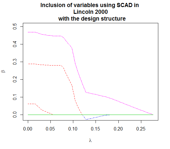
Turning our attention to the sparsity methods, we observe from Fig. 5.10(a) that the optimal value of is ; this indicates that the optimal number of parameters is 3. From Fig. 5.10(b), under SCAD, the variables chosen are , and . The model can be written as:
| (5.7) |
The coefficients of under SCAD were set to zero, but including in our SCAD analysis give us two extra terms compare to ().
We note here that all model selection techniques pick a different model list. picks the most complex model list, and pick a model list of size 27, pick a model of size 16 and SCAD pick a model of size 3. We also note that in (5.7) we have the interaction between and and their main effect. This is the first time that this occurs using shrinkage methods. The model given by SCAD is the best smallest model that we can have, however, the question is: Is this model the overall best model? I would say that this is not the overall best model because this model does not take into account the different type of varieties of wheat. (We comment that, here we have not used ALASSO because the R code we used did not support categorical variables.)
Analysis of Lincoln 2001 data with the design structure included in the model
| Size | ||||
|---|---|---|---|---|
| 1 | 16 | 31 | 42 | 284 |
| 2 | 12 | 4 | 7 | -783 |
| 3 | 10 | 3 | 5 | -943 |
| 4 | 16 | 10 | 16 | -239 |
| 5 | 16 | 10 | 16 | -234 |
| 6 | 15 | 10 | 16 | -234 |
| 7 | 14 | 7 | 11 | -441 |
| 8 | 11 | 3 | 5 | -922 |
| 9 | 12 | 3 | 6 | -924 |
| Size | ||||
|---|---|---|---|---|
| 10 | 11 | 3 | 6 | -918 |
| 11 | 12 | 3 | 6 | -913 |
| 12 | 9 | 3 | 4 | -1000 |
| 13 | 9 | 3 | 4 | -1000 |
| 14 | 9 | 3 | 4 | -992 |
| 15 | 9 | 3 | 4 | -986 |
| 16 | 9 | 3 | 4 | -980 |
| 17 | 8 | 3 | 4 | -981 |
| 18 | 42 | 3 | 19 | -1452 |
| Size | ||||
|---|---|---|---|---|
| 19 | 32 | 3 | 7 | -1853 |
| 20 | 32 | 3 | 7 | -1831 |
| 21 | 32 | 2 | 3 | -1826 |
| 22 | 28 | 3 | 7 | -1829 |
| 23 | 28 | 3 | 7 | -1823 |
| 24 | 28 | 3 | 7 | -1817 |
| 25 | 27 | 3 | 6 | -1819 |
| 26 | 27 | 3 | 6 | -1819 |
| 27 | 27 | 3 | 6 | -1819 |
Table 5.13 gives the estimate of , the values of , and in Lincoln 2001. In these cases, we included the design structure represented by the incomplete block.
We observe some a lot of variability in the estimate of : it takes on values from 8 to 42. The smallest discrepancy between the size of the conjectured model and occurs when the size of the conjectured model is 27. In fact, at that point . We also see that there is variability in the values of and as the size of the conjectured model increases. The smallest value of namely two, occurs first when the size of the conjectured model is 21. The smallest value of also occurs at the conjectured model of size 21. The smallest value of occurs with model of size 19.


Turning our attention to the sparsity methods, we observe from Fig. 5.11(a) that the optimal value of is ; this indicates that the optimal number of parameters is 3. From Fig. 5.10(b), under SCAD, the variable chosen is , and and the model can be written as:
| (5.8) |
This has the same explanatory variables as (5.7).
We note again that all model selection techniques pick a different model. picks a model with 19 variables, and pick a model of size 21, pick a model of size 27 and SCAD pick a model of size 3. We also note that in (5.8) we have the interaction between and and their main effects.
Overall, the model sizes range from 3 (SCAD), 19 (BIC), 21 ( and ) to 27 (). Since SCAD and BIC are sparsity or sparsity-like procedures, it is not surprising that they give the smallest models and unless a coarse model is desired, SCAD and possibly BIC can be ignored. In this example, we are left with models of size 21 and 27 and we recall that, compared to Bayes methods such as SCAD and BIC, our method is more sensitive to bias or, more precisely to exactly which variables are being included. We suspect that as in other cases, is even more sensitive than and and has detected that some variables are relevant when blocking in included. Indeed, the elevated size of shows how important the blocking is.
5.5 Analysis of Wheat data using SNP information
Our goal in this section is to see the effect of how taking the SNP (Single Nucleotide Polymorphism) information into account will affect the estimate of VCD. Since the variables representing the SNP’s have so much missing data, we imply dropped all rows with missing SNP values and only use SNP’s that are complete (No missing values i.e., we dropped columns as well.) Thus we retained only 6 SNP’s and our sample size was reduced to 2631. As before, we ordered the inclusion of covariates in our model using correlation. Under correlation is inclusion of terms in our model is as follows: . Here the SNP’s are symply denoted by their labels in the data. With this order, we fit 32 different models, each time, we estimate , find values of , and and models for , SCAD and ALASSO.
| Size | ||||
|---|---|---|---|---|
| 1 | 37 | 380 | 439 | 2381 |
| 2 | 37 | 193 | 235 | 587 |
| 3 | 37 | 185 | 226 | 477 |
| 4 | 37 | 181 | 222 | 430 |
| 5 | 36 | 37 | 55 | -3930 |
| 6 | 37 | 37 | 56 | -3924 |
| 7 | 37 | 8 | 17 | -9100 |
| 8 | 37 | 8 | 17 | -9093 |
| 9 | 36 | 8 | 16 | -9089 |
| 10 | 36 | 8 | 16 | -9081 |
| Size | ||||
|---|---|---|---|---|
| 11 | 36 | 8 | 16 | -9074 |
| 12 | 36 | 8 | 16 | -9066 |
| 13 | 36 | 8 | 16 | -9058 |
| 14 | 36 | 8 | 16 | -9052 |
| 15 | 36 | 8 | 16 | -9045 |
| 16 | 36 | 8 | 16 | -9040 |
| 17 | 36 | 8 | 16 | -9033 |
| 18 | 36 | 8 | 16 | -9026 |
| 19 | 36 | 8 | 16 | -9019 |
| 20 | 36 | 8 | 16 | -9014 |
| Size | ||||
|---|---|---|---|---|
| 21 | 36 | 8 | 16 | -9006 |
| 22 | 36 | 8 | 16 | -8999 |
| 23 | 41 | 8 | 17 | -8993 |
| 24 | 41 | 8 | 17 | -8989 |
| 25 | 41 | 8 | 17 | -8982 |
| 26 | 41 | 8 | 17 | -8978 |
| 27 | 41 | 8 | 17 | -8970 |
| 28 | 41 | 8 | 17 | -8962 |
| 29 | 41 | 8 | 17 | -8961 |
| 30 | 41 | 8 | 17 | -8956 |
| 31 | 41 | 8 | 17 | -8948 |
| 32 | 41 | 8 | 17 | -8940 |
Table 5.14 gives the estimate of , the values of , and . In these cases, we included the SNP’S variables.
We observe some variability in the estimate of : it takes values 36, 37, and 41. The smallest discrepancy between the size of the conjectured model and occurs when the size of the conjectured model is 32. In fact, at that point , suggests that the sample size may be low for our purpose here (We recall that model selection requires more data than parameter estimation). We also observe some variability in the values of and as the size of the conjectured model increases. There is a big drop in their value when the size of the conjectured model is 7, and thereafter, they become almost flat. The smallest value of , namely eight, and , namely 16, occur for models of size 7 and 9 respectively. The smallest value of occurs for model of size 8.


Turning our attention to the sparsity methods, we observe from Fig. 5.12(a) that the optimal value of is ; this indicates that the optimal number of parameters is 3. From Fig. 5.10(b), under SCAD, the variable chosen is , and and the model can be written as:
| (5.9) |
Similarly, using ALASSO we have,
| (5.10) |
So, (5.10) and (5.9) are identical. We also note that and pick the same variables. picks a model of size 9 (Large by one term), picks the most complex model, and SCAD and ALASSO pick a the smallest models, of size 3. We also note that in (5.9) and (5.10) we have the interaction between and and their main effects. As noted before, tends to be most sensitive to bias, so it is not surprising that it is the largest and includes all SNP’s. On the other hand, the first SNP to appear on the list is , on the list. This means SCAD, ALASSO, and choose no SNP’s. However, includes , and includes all the SNP’s that had no missing values. Moreover, being larger than 32 – the largest model size– suggests that other SNP’s that may have been excluded due to missing values, or other missing variables such as variety, may be critical to explain .
1
Chapter 6 General Conclusions and Future Work
In this Dissertation, we have developed a general method to estimate the VCD for classes of regression models.
Our method rests on minimizing an upper bound on an error. The upper bound depends on and generates an estimator . We have applied our method to a variety of linear regression problems. Our method is highly data driven and at least for linear regression models with large enough sample sizes, seems to give better results on simulated and real datasets in contrast with other established methods. Otherwise put, at a minimum, the models selected by our method are, on balance, no worse and often better than models selected by other methods such as , SCAD, ALASSO, and two forms of empirical risk minimization (). The comparison between and the ’s is not a surprise since the ’s are function of .
In Sec. 6.1, we review what the Dissertation has accomplished, and in Sec. 6.2, we identify gaps that remain to be filled and future work
6.1 General Conclusions
In Chapter 1, we reviewed the Vapnik-Chervonenkis concept of complexity often called a dimension here abbreviated . Since it is relatively unfamiliar to statisticians, we recalled the geometric, combinatorial and covering number definitions of . Then we summarized the work of Vapnik et al. Vapnik et al. (1994) and McDonald et al. McDonald et al. (2011) including the main theoretical results and the computational procedure.
All of this previous work was done for classification problems whereas our work generalizes it to regression problems. This led us to modify substantially not just the theory, but also the computing. Moreover we have had at various junctures to correct simplifying assumptions made by earlier authors so as to obtain good performance of the VCD as a model selection principle.
Chapter 2 presents the main mathematical results undergirding our methodology. Specifically, we convert a generic regression problem into classifications problems and apply corrected form of Vapnik et al to each of the problems. This gives us a bound on the Expected Maximum Difference between Two Empirical Losses (EMDBTEL) in term of , the correct VCD.
In Chapter 3, computational exploration showed this bound was not tight enough for good model selection. So we optimized the constant factor in the upper bound and changed the error criterion so it ressembled a cross-validation error rather than simply the difference between two models. We verified that the mathematics of Chapter 2 continued to hold with this change of the form of error.
The second major contribution of Chapter 3 was to correct the Vapnik et al Vapnik et al. (1994) computational procedure so it would accurately encapsulate the mathematical quantities the upper bound used. We denoted this estimate of by . Our improved procedure is more computationally demanding. But not terribly so in term of running time. Thus, in our extensive simulations with linear models, we found the new method gave good results compared to Vapnik’s original algorithm as well as compared to and two forms of Empirical Risk Minimization propose by Vapnik Vapnik (1998).
In Chapter 3 we also introduced the concept of ‘consistency at the true model’ to help identify how exactly our method should be used. Indeed, all our method give is an estimate of the of the data generator (DG). To obtain this estimate in practice, we must conjecture the data generator and compare the various ’s from the DG’s to the known true ’s from the DG’s. Thus using can always cut down a model list to a sub-list although in general does not by itself identify a DG. To get around this problem we used nested model lists where the VCD of the models increased with their size. For these cases, is able to give a unique model, apart from random variability – which can be considerable.
Our used of required the selection of design points to use in a non-linear regression. Different design points lead to different values of as seen in Chapter 3, however, we note a sample size effect: As increases it seems that
- 1.
the design points matter less and less and
- 2.
the accuracy of for selecting among nested models (with variables ordered for inclusion only by their absolute correlation with the response or by the order of inclusion using SCAD) increases.
In chapter 4, we estimated using the Tour De France Dataset. We fitted two set of models. The first set is based on the following covariates , and , the second contains , and (Definitions and notations as in Chapter 4). Whichever of the two model lists is chosen, . That is, the best model to predict the average speed of the winner of the Tour De France dataset should have variables. We conclude that the better model list is the one containing , , , .
Our analysis in this example is exhaustive so we can get an indication of how our method performs relative to and two forms of ERM. We emphasize that although this chapter uses real datasets it is really a sort of ‘toy’ problem since the sample size is not large compared to the number of inferences we want to make.
In chapter 5, we implemented our method on more complex data sets. We also performed sparsity driven analyses, using SCAD and ALASSO in addition to estimating , and finding , and . We examined 2 datasets that are commonly regarded as ‘difficult’ or complex. We started with the Abalone dataset and found no matter the conjectured linear model. However, there were only 7 variables since we only used first order models. We observed that SCAD and ALASSO picked the same variables, but the estimated coefficient for these variables were extremely different from the two models, this may be due to the high correlation between covariates. These models included but not , whereas the models chosen by , and included but not . That is, the sparsity methods led to the same variables, and , and used the same variables (albeit a different set) while included all the variables, suggesting that some variables are missing i.e there is unavoidable bias. We regard the model chosen by as the most reasonable because of the non-linear relationship between the response and the explanatory variables.
The second dataset that we used was the wheat dataset. We performed the estimation of using our method by location first and second we combined all locations to perform a multilocation analysis. Overall, we see that complexity varies from one location to another; this can be observed
by looking at the estimated , and the ordering of the variables in the models. The least complex location is Lincoln 2000 since the
for all model lists. We also observe that
was the most important variable no matter which location you choose and also had the highest correlation with yield.
Thus, we provide a complete analysis for all 7 locations using the phenotypic variables. Then we turned to two other analyses. The first used the phenotypic variables and the design structure variables, the second used the phenotypic variables and the SNP variables. That is we have shown how our method extends to models permitting two data types. In both cases, we found that the results were more complex that with uni-type datasets and that some SNP’s and some design variable were important to include. We could have done multi-type data analysis including phenotypic variables, design variables and SNP variables, but lacked of time to complete this. We note that the Wheat dataset has other variables in it e.g., variety, that we did not use. However, using them might have made the effective sample size too small relative to the model classes we wanted to use.
Over all, we found that our estimated VCD had higher values for real datasets than our comparably sized synthetic datasets indicating was in fact reflecting the complexity of the DG. Moreover, in all cases, gave results that were reasonable even when other methods gave models that were obviously too parsimonious or otherwise implausible. We attribute this to the sensitivity of to bias. By contrast, often other methods have some level of built-in-sparsity so they give smaller models than are reasonable.
As a pragmatic recommendation, we therefore suggest that for complex datasets having a large enough that the conjecture model to be nested and the model selected by be compared with the model selected by other methods. That is, we think that no one method for model selection is the method to use. We think that judicious comparison of models selected unless different principles (sparsity, small bias, complexity, etc) is the appropriate way to do model selection. In this context, our method is simply another well performing method whose output should be taken into consideration for optimal model building.
6.2 Future Work
No Dissertation can solve all the problems related to a new methodology and this Dissertation is no exception.. There are (at least) five problems that we would like to address in future developing the VCD for model selection.
- 1.
As it stands, come from optimizing an upper bound. It is not clear how to re-do the analysis leading to the upper bound so as to derive a variance for . At the present, we can only suggest using a bootstrap approach: form from bootstrap samples and then form from them.
- 2.
We have limited our work to linear models although our general theory applies to any class of regression models for which VCD’s can be calculated. This includes Trees, Kernel methods, and neural networks, amongst others. These classes are more complicated but being non-linear may give better results in real problems.
- 3.
A theoretical gap in our derivation in Chapter 2 is that we only have an upper bound on the EMDBTEL. We have tried to make it tight computationally, but having either a provably tight upper bound on the EMDBTEL or a provably tight lower bound on the EMDBTEL would make our inferences more convincing.
- 4.
Another theoretical gap is to prove in probability. McDonald et al McDonald et al. (2011) tried to do this in the classification case but there are some gaps in their proof: For instance, they have a bound for the sum of absolute errors but they want a bound for the absolute error of the sum. We run into the exact same problem when we adapt their proof to regression, see Appendix A.4. However we think we have overcome it.
- 5.
Although, we have shown in an example (see 5.4, 5.5) how our method can be used for two data types with linear models, the general question of how well our method performs in comparison to other methods for multi-type data remains to be explored. The issue is that as more data types become available the modeling becomes more complex and may outstrip ’s ability to scale up with the number of data types and overall sample sizes.
Obviously, this list is not complete, but it may serve as a warning that however well our method seems to perform in preliminary heats, reasonable questions about it remain to be answered before it is ready for general use.
Appendix A CHAPTER 2 APPENDIX
A.1 Proof of Theorem 2.2.1 clause 1
A.2 Proof of Theorem 2.2.1 clause 2
We will first state and proof the following Lemma
Lemma A.2.1.
Let . The probability of the supremal difference between two empirical losses using cross-validation form of the error is bounded above by
| (A.7) |
Proof.
The LHS is bounded by
if
∎
Proposition A.2.1.
Let , where is unbounded, be the sample size. If , and
where is some fixed parameter, we have
| (A.8) |
where .
Proof.
By Lemma A.2.1, we have
| (A.9) |
| (A.10) |
Each probability on the right hand side of (A.10) can be bounded. Since is a maximum, we have . Thus, for either the positive or negative parts in (A.10) we have
Letting and using Theorem 2.1.1, Clause 3, the last inequality gives
| (A.11) |
Using (A.11), both terms on the right in (A.10) can be bounded. This gives
| (A.12) |
The presence of in the the exponent of the hannealed entropy will not change the validity of Clause I of Theorem 2.1.1, so we have, therefore, Using this in (A.12) gives
Recalling the extra factor of 2 in inequality (A.9) gives the statement of the Proposition. ∎
Now let prove Theorem 2.2.1 clause 2.
A.3 Proof of Theorem 2.2.1 clause 3
A.4 Proof of Consistency
Here, we offer a proof of consistency of to . In almost all respects this tentative of proof should be credited to McDonald et al. (2011). Our contribution is the examination of the gaps in their proof. Our two ugly hypotheses and the discussion about how to satisfy them fill the gaps in their proof. We have put it in as appendix rather than the main part of the thesis because we have not finished verifying all the details satisfactorily. Instead, we have not convince ourselves it is error free. Nevertheless, we have the following. ’s represent the ’s in Algorithm 2
Lemma A.4.1.
Let and let , where ’s are independent for any given ’s. Then at any design point , we have
| (A.16) |
Proof.
Fix . Now, for any and , and , using Hoeffding’s lemma we have
Thus, we have
| (A.17) | |||||
∎
Proposition A.4.1.
Suppose that is a set of random variables satisfying Lemma A.4.1. Then for any and , we have
| (A.18) |
Proof.
Definition A.4.1.
. For let be the minimal -covering set of So and for each , there exists a such that . We choose , since . The key argument is based on the entropy of the restricted class . is defined as follows:
| (A.21) |
We assume without any proof that the following theorem is true.
Theorem A.4.1.
Let assume that we have a collection of functions inside so that , where is an increasing function of .
Corollary A.4.1.
| (A.23) |
Proof.
| (A.24) |
| (A.25) |
So since the and are continuous, and if is large enough, using Def. A.4.1 and Theorem A.4.1 we have
| (A.26) |
Using A.26, we have
| (A.27) |
Let be a positive number satisfying , and using A.27, we have
| (A.29) |
Using A.22, we have
| (A.30) |
∎
Theorem A.4.2.
Let
| (A.31) |
and suppose that . Then,
| (A.32) |
References
- Aba (1996) Abalone data set. https://archive.ics.uci.edu/ml/machine-learning-databases/abalone/?C=D;O=D, 1996.
- Anthony and Bartlett (2009) M. Anthony and P. L. Bartlett. Neural network learning: Theoretical foundations. cambridge university press, 2009.
- Berk et al. (2013) R. Berk, L. Brown, A. Buja, K. Zhang, L. Zhao, et al. Valid post-selection inference. The Annals of Statistics, 41(2):802–837, 2013.
- Campbell et al. (2003) B. Campbell, P. S. Baenziger, K. Gill, K. M. Eskridge, H. Budak, M. Erayman, I. Dweikat, and Y. Yen. Identification of qtls and environmental interactions associated with agronomic traits on chromosome 3a of wheat. Crop Science, 43(4):1493–1505, 2003.
- Clyde and George (2004) M. Clyde and E. I. George. Model uncertainty. Statistical science, pages 81–94, 2004.
- Devroye (1996) L. Devroye. Gy orfi, l., lugosi, g., 1996. a probabilistic theory of pattern recognition. Applications of mathematics, 31, 1996.
- Devroye et al. (2013) L. Devroye, L. Györfi, and G. Lugosi. A probabilistic theory of pattern recognition, volume 31. Springer Science & Business Media, 2013.
- Draper (1995) D. Draper. Assessment and propagation of model uncertainty. Journal of the Royal Statistical Society. Series B (Methodological), pages 45–97, 1995.
- Ebrahimi et al. (1999) N. Ebrahimi, E. Maasoumi, and E. S. Soofi. Ordering univariate distributions by entropy and variance. Journal of Econometrics, 90(2):317–336, 1999.
- Ebrahimi et al. (2010) N. Ebrahimi, E. S. Soofi, and R. Soyer. On the sample information about parameter and prediction. Statistical Science, pages 348–367, 2010.
- Efron et al. (2004) B. Efron, T. Hastie, I. Johnstone, R. Tibshirani, et al. Least angle regression. The Annals of statistics, 32(2):407–499, 2004.
- Fan and Li (2001) J. Fan and R. Li. Variable selection via nonconcave penalized likelihood and its oracle properties. Journal of the American Statistical Association, 96(456):1348–1360, 2001. doi: 10.1198/016214501753382273. URL http://dx.doi.org/10.1198/016214501753382273.
- Fan and Lv (2008) J. Fan and J. Lv. Sure independence screening for ultrahigh dimensional feature space. Journal of the Royal Statistical Society: Series B (Statistical Methodology), 70(5):849–911, 2008.
- McDonald (2012) D. McDonald. Generalization error bounds for time series. phd thesis, department of statistics, carnegie-mellon university, 2012.
- McDonald et al. (2011) D. J. McDonald, C. R. Shalizi, and M. Schervish. Estimated vc dimension for risk bounds. arXiv preprint arXiv:1111.3404, 2011.
- Moore (2001) A. W. Moore. Vc-dimension for characterizing classifiers. Tutorial at http://www-2. cs. cmu. edu/awm/tutorials/vcdim08. pdf, 2001.
- Pollard (1984) D. Pollard. Convergence of Stochastic Processes. Springer-Verlag, New York, 1984.
- Sauer (1972) N. Sauer. On the density of families of sets. Journal of Combinatorial Theory, Series A, 13(1):145–147, 1972.
- Shao (1993) J. Shao. Linear model selection by cross-validation. Journal of the American statistical Association, 88(422):486–494, 1993.
- Shao et al. (2000) X. Shao, V. Cherkassky, and W. Li. Measuring the vc-dimension using optimized experimental design. Neural computation, 12(8):1969–1986, 2000.
- Soofi (1994) E. S. Soofi. Capturing the intangible concept of information. Journal of the American Statistical Association, 89(428):1243–1254, 1994.
- van de Geer (2000) S. van de Geer. Empirical processes in m-estimation. cambridge series in statistical and probabilistic mathematics, 2000.
- Van Der Vaart and Wellner (1996) A. W. Van Der Vaart and J. A. Wellner. Weak Convergence. Springer, 1996.
- Van der Waart (1998) A. Van der Waart. Asymptotic statistics, volume 27 of cambridge series in statistical and probabilistic mathematics 03, 1998.
- Vapnik and Chervonenkis (1971) A. Vapnik and A. Chervonenkis. On the uniform convergence of relative frequencies to their probabilities. In Soviet Math. Dokl, volume 9, pages 915–918, 1971.
- Vapnik (1998) V. Vapnik. Statistical learning theory. 1998, 1998.
- Vapnik (1999) V. Vapnik. An overview of statistical learning theory. Neural Networks, IEEE Transactions on, 10(5):988–999, 1999.
- Vapnik and Chervonenkis (1968) V. Vapnik and A. Chervonenkis. On the uniform convergence of relative frequencies of events to their probabilities. In Soviet Math. Dokl, volume 9, pages 915–918, 1968.
- Vapnik et al. (1994) V. Vapnik, E. Levin, and Y. Le Cun. Measuring the vc-dimension of a learning machine. Neural Computation, 6(5):851–876, 1994.
- Vapnik and Chervonenkis (1991) V. N. Vapnik and A. J. Chervonenkis. The necessary and sufficient conditions for consistency of the method of empirical risk. Pattern Recognition and Image Analysis, 1(3):284–305, 1991.
- Zou (2006) H. Zou. The adaptive lasso and its oracle properties. Journal of the American statistical association, 101(476):1418–1429, 2006.
- Zou and Hastie (2005) H. Zou and T. Hastie. Regularization and variable selection via the elastic net. Journal of the Royal Statistical Society: Series B (Statistical Methodology), 67(2):301–320, 2005.