Multiple Disk Gaps and Rings Generated by a Single Super-Earth:
II. Spacings, Depths, and Number of Gaps, with Application to Real Systems

The Atacama Large Millimeter Array (ALMA) has discovered multiple gaps and rings in a number of protoplanetary disks in dust continuum emission at millimeter (mm) wavelengths at $\sim$10–100 AU. Examples include the disk around HL Tau [3], TW Hya [4, 83], HD 163296 [42], AS 209 [31], AA Tau [55], Elias 24 [13, 15, 21], GY 91 [74], and V1094 Sco [5, 85]. The origins of these gaps are being debated. Several hypotheses have been put forward, including disk-planet interaction [26, 20, 64, 43, e.g.,], zonal flows [63], secular gravitational instability [79, e.g.,], self-induced dust pile-ups [39], radially variable magnetic disk winds [76, 77], and dust sintering and evolution at snowlines [91, 60]. In nearly all mechanisms, perturbations in gas are followed by radial drift and concentration of mm-sized dust [86, 11, 93, e.g.,]. In planet-disk interaction scenarios, even super-Earth planets may open dust gaps [95, 72, 19, 18, e.g.,].

At first glance, multiple gaps seem to imply multiple planets, with one planet embedded within each gap. Recently, however, it has been appreciated that a single planet can generate multiple gaps. Using gas+dust simulations, Dong et al. [23] showed that one super-Earth planet (with mass between Earth and Neptune) can produce up to five dust gaps in a nearly inviscid disk, and that these gaps would be detectable by ALMA (see also Muto et al. 59, Duffell & MacFadyen 29, Zhu et al. 94, Bae et al. 8, Chen & Lin 12, Ricci et al. 70). In particular, a pair of closely spaced narrow gaps (a “double gap”) sandwiches the planet’s orbit. This structure is created by the launching, shocking, and dissipation of two primary density waves, as shown in Goodman & Rafikov [40, see also ]. Additional gaps interior to the planet’s orbit may also be present, possibly opened by the dissipation of secondary and tertiary density waves excited by the planet [6, 7].

Motivated by the boom of multi-gap structures discovered by ALMA, and the mounting evidence of extremely low levels of turbulence at the disk midplane (from direct gas line observations, e.g., Flaherty et al. 32, Flaherty et al. 33, Teague et al. 82, and from evidence for dust settling, e.g., Pinte et al. 65, Stephens et al. 75), we investigate here what properties of the planet and disk can be inferred from real-life gap observations. We study systematically how gap properties depend on planet and disk parameters, and propose generic guidelines connecting ALMA observations with disk-planet interaction models. We introduce our models in §II, and present our main parameter survey of gap properties in §III. These results are applied to three actual disks in §IV, discussed in §V, and summarized in §VI.

We use two-fluid (gas + dust) 2D hydrodynamics simulations in cylindrical coordinates (radius $r$ and azimuth $\phi$) to follow the evolution of gas and dust in a disk containing one planet. The code used is LA-COMPASS (Li et al. 50, Li et al. 51). The numerical setup, largely adopted from Dong et al. [23], is summarized here (more details can be found in Fu et al. 34 and Miranda et al. 57).

We adopt a locally isothermal equation of state: pressure $P=\Sigma_{\rm gas}c_{\rm s}^{2}$, where $\Sigma_{\rm gas}$ and $c_{\rm s}$ are the surface density and sound speed of the gas. Dust is modeled as a pressureless second fluid. The following Navier-Stokes equations are solved:

where $D_{\rm dust}$ is the dust diffusivity defined as $D_{\rm dust}=\nu/(1+\tau_{\rm stop}^{2})$ [80], $\Phi_{\rm G}$ is the gravitational potential (including both the gravity of the planet and the self-gravity of the disk; a smoothing length of 0.7$h$ is applied to the gravitational potential of the planet), $\mathbf{f}_{\rm drag}=\frac{\Omega_{\rm K}}{\tau_{\rm stop}}(\mathbf{v}_{\rm gas}-\mathbf{v}_{\rm dust})$ is the drag force on dust by gas, $\tau_{\rm stop}$ is the dimensionless stopping time (see below), and $\mathbf{f}_{\nu}$ is the Shakura-Sunyaev viscous force with $\nu=\alpha h^{2}\Omega_{\rm K}$, $h$ the disk scale height, $\Omega_{\rm K}$ the Keplerian angular frequency, and $\alpha<1$ a dimensionless constant. Other symbols have their usual meanings. The last term in Eqn. (3) accounts for the dust back-reaction on gas.

The initial surface densities of gas and dust are (we use the subscript 0 to indicate initial conditions):

where $r_{\rm p}=30$ AU is the radius of the planet’s circular orbit, which is fixed in our simulations. We note that if a planet migrates in the radial direction fast enough, gap properties can be affected [23, Fig. 14]. However, low-mass planets in near-invicsid environments as studied here are not expected to migrate significantly [51, 90, 35]. We ramp up the planet mass with time $t$ as $M_{\rm p}(t)\propto\sin{(t)}$ over 10 orbits. In Dong et al. [23, Fig. 6] we experimented with different planet growth timescales up to a few thousand orbits, and found no significant effects on the rings and gaps ultimately produced by the planet.

The disk aspect ratio $h/r$ is assumed radially invariant. We adopt a constant instead of a flared $h/r$ profile to suppress the dependences of gap properties on the $h/r$ gradient, and to increase the timestep at the inner boundary. We note that fractional gap spacings, which we will use as our primary diagnostic of models and observations (see our equation 8), depend only weakly on radial gradients in $h/r$, $\Sigma_{\rm gas,0}$, and the slope of the background $\Sigma_{\rm gas}(r)$ profile. Dong et al. [23, Fig. 8] showed that as the background $\Sigma_{\rm gas}(r)$ profile varies from $\Sigma_{\rm gas}\propto r^{0}$ to $\Sigma_{\rm gas}\propto r^{-1.5}$, all gaps and rings shift inward, while their relative separations are unchanged at the level of a few percent.

The dimensionless stopping time of dust — the particle momentum stopping time normalized to the dynamical time — is, in the Epstein drag regime,

where $\rho_{\rm particle}=1.2$ g cm^-3 is the internal density of dust particles, and $s=0.2$ mm is the particle size. Such particles are probed by continuum emission at mm wavelengths [46, e.g.,]. At $r=0.2$–$1\,r_{\rm p}$, $\tau_{\rm stop}$ is on the order of 0.01. We note that for mm-to-cm sized particles often traced by VLA cm continuum observations (possibly having $\tau_{\rm stop}\sim 0.1-1$), gaps and rings similar to those in 0.2 mm sized dust are generated. Qualitatively, as particle size increases, gaps widen and deepen with their locations largely unchanged; the amplitude of the middle ring (MR) co-orbital with the planet drops; particle concentrations at the triangular Lagrange points L₄ and L₅ become stronger; and an azimuthal gap centered on the planet’s location emerges and widens [56, 95, 72, 70].

The simulation domain runs from 0 to $2\pi$ in $\phi$, and 0.1 to 2.1$r_{\rm p}$ in $r$. The initial gas disk mass is $0.015M_{\odot}$. We set up a wave damping zone at $r=0.1$–$0.2r_{\rm p}$ as described in de Val-Borro et al. [16], and an inflow boundary condition at the outer boundary. The resolution is discussed in §II.1.

We summarize our models in Table 1. The model name indicates the values of $h/r$ and $M_{\rm p}/M_{\rm th}$ adopted (e.g., in Model H003MP02, $h/r=0.03$ and $M_{\rm p}=0.2M_{\rm th}$). In all cases the planet mass $M_{\rm p}$ is lower than the disk thermal mass $M_{\rm th}=M_{\star}(h/r)^{3}$ ($M_{\star}=M_{\odot}$ is the stellar mass); the size of the planet’s Hill sphere is comparable to $h$ when $M_{\rm p}=M_{\rm th}$. An extremely low viscosity is necessary to enable low-mass planets to open gaps. We adopt $\alpha=5\times 10^{-5}$ for models with $M_{\rm p}>0.1M_{\rm th}$, where $\alpha$ is the Shakura & Sunyaev parameter characterizing the disk viscosity; in those models with $M_{\rm p}\leq 0.1M_{\rm th}$, we use even lower viscosities $\alpha=10^{-6}$–$10^{-5}$ to speed up gap opening [36, cf.,].

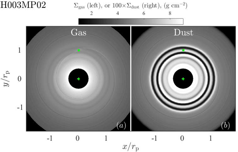
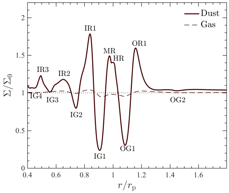
Figure 1 shows the 2D gas and dust distributions and their azimuthally averaged 1D radial profiles for Model H003MP02 at 1600 orbits (0.26 Myr at 30 AU). A $0.2M_{\rm th}=1.8M_{\oplus}$ planet produces multiple gaps and rings in both gas and dust, while the surface density perturbations in dust are an order of magnitude larger than they are in gas. In each of the dust rings, a few Earth masses of dust are trapped. We refer to the gaps and rings inside $r_{\rm p}$ as “inner” gaps and rings (IG and IR), and the ones outside $r_{\rm p}$ as “outer” gaps and rings (OG and OR), and number them according to their distances from the planet.

In this section, we study how the properties of gaps and rings vary with input parameters. Most simulations are run for $\sim$10³–$10^{4}$ orbits ($\sim$0.1–1 Myr at 30 AU), after which time dust gaps are depleted by a factor of $\sim$2–10 in surface density, reminiscent of observed gap depths [e.g., 3, 4, of course, observed gap depths are measured in units of surface brightness]. Dust gaps in our simulations do not have detectable eccentricities. The locations of gaps and rings, $r_{\rm gap}$ and $r_{\rm ring}$, are defined as the radii at which $\Sigma_{\rm dust}/\Sigma_{\rm dust,0}$ attains local minima and maxima, respectively; only robust (non-transient) features are counted. The relative separation (spacing) between two radii (as drawn from $r_{\rm gap}$, $r_{\rm ring}$, or $r_{\rm p}$) is defined as

In real observations, $r_{\rm p}$ is usually unknown, and the spacings of gaps and rings are the direct observables.

In this section, we make a quick comparison between our models and observed disks, focussing on those having three or more narrow gaps in mm continuum emission (HL Tau, TW Hya, and HD 163296). These comparisons do not involve detailed fits. Rather, the models are taken directly from our parameter survey grid, and are not specifically tailored to the observations. We focus on gap locations and not on gap depths for reasons discussed in §III.1. We begin by picking $h/r$ consistent with disk midplane temperatures, $T_{\rm midplane}$, as derived from the literature. We then identify a pair of gaps as the “double gap”. For HL Tau and TW Hya, this is the most compact pair, and for HD 163296, it is the pair farthest from the star. The midline of the double gap locates the planet position $r_{\rm p}$. We then estimate $M_{\rm p}$ using Eqn. (10), selecting the one model from our grid that appears to best reproduce the double gap locations. A non-trivial test of the model is to see whether it can reproduce the locations of observed gaps interior to the double gap.

The observed surface brightness radial profiles $I_{\rm mm}(r)$ are shown in Figure 8, with modelled planet and gap locations indicated. We mark all modelled gaps at $r\geq 0.4r_{\rm p}$ regardless of their depths, but do not show the model surface brightness radial profile, again because our intent is not to fit gap depths. We attempt to remove the dependence of $I_{\rm mm}$ on dust temperature by scaling $I_{\rm mm}$ by $\sqrt{r}$.

Figure 9 shows side-by-side comparisons of observations with synthetic model ALMA continuum images, produced using radiative transfer simulations using the Whitney et al. [87] code. The procedures are described in Dong et al. [26, see also ]. Briefly, 2D hydro disk structures are inflated into 3D, assuming hydrostatic equilibrium with each model’s $h/r$. Starlight is reprocessed to longer wavelengths at the disk surface by a population of “small” (sub-$\mu$m-sized) interstellar medium dust (Kim et al. 47). These small grains are assumed to be well-coupled to gas with a volumetric mass density equal to 10^-2 that of the gas. A population of “big” dust particles (representing the second fluid in hydro simulations) is assumed to have settled to the midplane with a Gaussian vertical density profile and a scale height equal to $h_{\rm dust}=0.1h$, in line with $h_{\rm dust}$ estimated in real disks [65, e.g., HL Tau, $\sim$1% at 100 AU;]. The optical properties of the small dust can be found in Dong et al. [27, Fig. 2]. The big dust is assumed to have an opacity $\kappa=3.5$ cm² g^-1 at 870 $\micron$. For the central source we assume a 1$M_{\odot}$ pre-main-sequence star with $R_{\star}=2.4R_{\odot}$ and $T_{\star}=4400$K. Radiative transfer simulations produce synthetic images of continuum emission at 870 $\micron$, which are processed using the simobserve and simanalyze tools in Common Astronomy Software Applications (CASA) to simulate ALMA images with 4-hour integration times and default settings.

We carry out two-dimensional, two-fluid hydrodynamical simulations of protoplanetary disks with low viscosities ($\alpha\lesssim 10^{-4}$) to study the spacings, depths, and total number of dust gaps opened by one sub-thermal mass planet ($M_{\rm p}<M_{\rm th}=M_{\star}(h/r)^{3}$). Our results provide basic guidelines for interpreting multi-gap structures seen in mm continuum emission. Our main findings are:

1. 1.

   Among the observable properties of gaps and rings, gap location is the least affected by observing conditions, finite optical depth, and time evolution (§III.1; §III.2; Figure 4).

2. 2.

   Gap spacings increase with increasing $h/r$ and decreasing $M_{\rm p}$ (§III.3; Figure 5). We provide empirical fitting functions for the double gap OG1+IG1 (defined in Figure 1; Eqn. 10) and IG2 (Eqn. 11; Figure 6).

3. 3.

   Gaps are opened faster by planets with higher masses, and in disks with higher $h/r$ (§III.4).

4. 4.

   More gaps are opened within a given radius range in disks with lower $h/r$. The number of gaps is less sensitive to $M_{\rm p}$.

5. 5.

   The spacings of the double gap in HL Tau [3] and TW Hya [4], and all three gaps in HD 163296 [42] match those of modelled gaps produced by a sub-Saturn mass planet (§IV; Figures 8 and 9).

6. 6.

   A low midplane viscosity ($\alpha\lesssim 10^{-4}$) is needed for a sub-thermal mass planet to open multiple gaps (Figure 10). The Rossby wave instability may develop at the edges of gaps, producing multiple dusty vortices (Figure 11). A planet as low mass as Mars may significantly perturb the dust disk in terrestrial planet forming regions (Figure 12).

We are grateful to an anonymous referee for constructive suggestions that improved our paper. We thank David Bennett, Jeffrey Fung, Frederic Masset, Roman Rafikov, Satoshi Okuzumi, and Wei Zhu for discussions, and Eiji Akiyama, Sean Andrews, Crystal Brogan, Giovanni Dipierro, Davide Fedele, Jane Huang, Andrea Isella, and Ryan Loomis for making the ALMA images available. This research used the SAVIO computational cluster at UC Berkeley, as facilitated by Paul Kalas. H.L. and S.L. gratefully acknowledge support by the NASA/ATP and LANL/Center for Space and Earth Science programs.

References

- [1] Akiyama, E., Hasegawa, Y., Hayashi, M., & Iguchi, S. 2016, ApJ, 818, 158
- [2] Akiyama, E., Muto, T., Kusakabe, N., et al. 2015, ApJ, 802, L17
- [3] ALMA Partnership, Brogan, C. L., Pérez, L. M., et al. 2015, ApJ, 808, L3
- [4] Andrews, S. M., Wilner, D. J., Zhu, Z., et al. 2016, ApJ, 820, L40
- [5] Ansdell, M., Williams, J. P., Trapman, L., et al. 2018, ArXiv e-prints, arXiv:1803.05923
- [6] Bae, J., & Zhu, Z. 2018a, ApJ, 859, 118
- [7] —. 2018b, ApJ, 859, 119
- [8] Bae, J., Zhu, Z., & Hartmann, L. 2017, ApJ, 850, 201
- [9] Bai, X.-N. 2015, ApJ, 798, 84
- [10] Bai, X.-N., & Stone, J. M. 2013, ApJ, 769, 76
- [11] Birnstiel, T., Dullemond, C. P., & Brauer, F. 2010, A&A, 513, A79
- [12] Chen, J.-W., & Lin, M.-K. 2018, MNRAS, arXiv:1805.00940
- [13] Cieza, L. A., Casassus, S., Pérez, S., et al. 2017, ApJ, 851, L23
- [14] Cox, A. W., Grady, C. A., Hammel, H. B., et al. 2013, ApJ, 762, 40
- [15] Cox, E. G., Harris, R. J., Looney, L. W., et al. 2017, ApJ, 851, 83
- [16] de Val-Borro, M., Edgar, R. G., Artymowicz, P., et al. 2006, MNRAS, 370, 529
- [17] Debes, J. H., Poteet, C. A., Jang-Condell, H., et al. 2017, ApJ, 835, 205
- [18] Dipierro, G., & Laibe, G. 2017, MNRAS, 469, 1932
- [19] Dipierro, G., Laibe, G., Price, D. J., & Lodato, G. 2016, MNRAS, 459, L1
- [20] Dipierro, G., Price, D., Laibe, G., et al. 2015, MNRAS, 453, L73
- [21] Dipierro, G., Ricci, L., Pérez, L., et al. 2018, MNRAS, 475, 5296
- [22] Dong, R., & Fung, J. 2017, ApJ, 835, 146
- [23] Dong, R., Li, S., Chiang, E., & Li, H. 2017, ApJ, 843, 127
- [24] Dong, R., Rafikov, R. R., & Stone, J. M. 2011a, ApJ, 741, 57
- [25] Dong, R., Rafikov, R. R., Stone, J. M., & Petrovich, C. 2011b, ApJ, 741, 56
- [26] Dong, R., Zhu, Z., & Whitney, B. 2015, ApJ, 809, 93
- [27] Dong, R., Rafikov, R., Zhu, Z., et al. 2012, ApJ, 750, 161
- [28] Dong, R., Liu, S.-y., Eisner, J., et al. 2018, ApJ, 860, 124
- [29] Duffell, P. C., & MacFadyen, A. I. 2012, ApJ, 755, 7
- [30] Fairlamb, J. R., Oudmaijer, R. D., Mendigutía, I., Ilee, J. D., & van den Ancker, M. E. 2015, MNRAS, 453, 976
- [31] Fedele, D., Tazzari, M., Booth, R., et al. 2018, A&A, 610, A24
- [32] Flaherty, K. M., Hughes, A. M., Rosenfeld, K. A., et al. 2015, ApJ, 813, 99
- [33] Flaherty, K. M., Hughes, A. M., Rose, S. C., et al. 2017, ApJ, 843, 150
- [34] Fu, W., Li, H., Lubow, S., Li, S., & Liang, E. 2014, ApJ, 795, L39
- [35] Fung, J., & Chiang, E. 2017, ArXiv e-prints, arXiv:1701.08161
- [36] Fung, J., Shi, J.-M., & Chiang, E. 2014, ApJ, 782, 88
- [37] Gaia Collaboration, Brown, A. G. A., Vallenari, A., et al. 2018, ArXiv e-prints, arXiv:1804.09365
- [38] Garufi, A., Quanz, S. P., Schmid, H. M., et al. 2014, A&A, 568, A40
- [39] Gonzalez, J.-F., Laibe, G., Maddison, S. T., Pinte, C., & Ménard, F. 2015, MNRAS, 454, L36
- [40] Goodman, J., & Rafikov, R. R. 2001, ApJ, 552, 793
- [41] Huang, J., Andrews, S. M., Cleeves, L. I., et al. 2018, ApJ, 852, 122
- [42] Isella, A., Guidi, G., Testi, L., et al. 2016, Physical Review Letters, 117, 251101
- [43] Jin, S., Li, S., Isella, A., Li, H., & Ji, J. 2016, ApJ, 818, 76
- [44] Johansen, A., & Lambrechts, M. 2017, Annual Review of Earth and Planetary Sciences, 45, 359
- [45] Johansen, A., & Youdin, A. 2007, ApJ, 662, 627
- [46] Kataoka, A., Tsukagoshi, T., Pohl, A., et al. 2017, ApJ, 844, L5
- [47] Kim, S.-H., Martin, P. G., & Hendry, P. D. 1994, ApJ, 422, 164
- [48] Kwon, W., Looney, L. W., & Mundy, L. G. 2011, ApJ, 741, 3
- [49] Li, H., Colgate, S. A., Wendroff, B., & Liska, R. 2001, ApJ, 551, 874
- [50] Li, H., Li, S., Koller, J., et al. 2005, ApJ, 624, 1003
- [51] Li, H., Lubow, S. H., Li, S., & Lin, D. N. C. 2009, ApJ, 690, L52
- [52] Lin, J. W., Lee, E. J., & Chiang, E. 2018, ArXiv e-prints, arXiv:1806.00487
- [53] Liu, S.-F., Jin, S., Li, S., Isella, A., & Li, H. 2018, ApJ, 857, 87
- [54] Liu, Y., Henning, T., Carrasco-González, C., et al. 2017, A&A, 607, A74
- [55] Loomis, R. A., Öberg, K. I., Andrews, S. M., & MacGregor, M. A. 2017, ApJ, 840, 23
- [56] Lyra, W., Johansen, A., Klahr, H., & Piskunov, N. 2009, A&A, 493, 1125
- [57] Miranda, R., Li, H., Li, S., & Jin, S. 2017, ApJ, 835, 118
- [58] Monnier, J. D., Harries, T. J., Aarnio, A., et al. 2017, ApJ, 838, 20
- [59] Muto, T., Suzuki, T. K., & Inutsuka, S.-i. 2010, ApJ, 724, 448
- [60] Okuzumi, S., Momose, M., Sirono, S.-i., Kobayashi, H., & Tanaka, H. 2016, ApJ, 821, 82
- [61] Ormel, C. W. 2017, in Astrophysics and Space Science Library, Vol. 445, Astrophysics and Space Science Library, ed. M. Pessah & O. Gressel, 197
- [62] Perez-Becker, D., & Chiang, E. 2011, ApJ, 727, 2
- [63] Pinilla, P., Birnstiel, T., Ricci, L., et al. 2012, A&A, 538, A114
- [64] Pinilla, P., de Juan Ovelar, M., Ataiee, S., et al. 2015, A&A, 573, A9
- [65] Pinte, C., Dent, W. R. F., Ménard, F., et al. 2016, ApJ, 816, 25
- [66] Poleski, R., Skowron, J., Udalski, A., et al. 2014, ApJ, 795, 42
- [67] Rafikov, R. R. 2002a, ApJ, 569, 997
- [68] —. 2002b, ApJ, 572, 566
- [69] Rapson, V. A., Kastner, J. H., Millar-Blanchaer, M. A., & Dong, R. 2015, ApJ, 815, L26
- [70] Ricci, L., Liu, S.-F., Isella, A., & Li, H. 2018, ApJ, 853, 110
- [71] Rosenfeld, K. A., Andrews, S. M., Hughes, A. M., Wilner, D. J., & Qi, C. 2013, ApJ, 774, 16
- [72] Rosotti, G. P., Juhasz, A., Booth, R. A., & Clarke, C. J. 2016, MNRAS, 459, 2790
- [73] Schlaufman, K. C. 2018, ApJ, 853, 37
- [74] Sheehan, P. D., & Eisner, J. A. 2018, ApJ, 857, 18
- [75] Stephens, I. W., Yang, H., Li, Z.-Y., et al. 2017, ApJ, 851, 55
- [76] Suriano, S. S., Li, Z.-Y., Krasnopolsky, R., & Shang, H. 2017a, MNRAS, 468, 3850
- [77] —. 2017b, ArXiv e-prints, arXiv:1712.06217
- [78] Suzuki, D., Bennett, D. P., Sumi, T., et al. 2016, ApJ, 833, 145
- [79] Takahashi, S. Z., & Inutsuka, S.-i. 2014, ApJ, 794, 55
- [80] Takeuchi, T., & Lin, D. N. C. 2002, ApJ, 581, 1344
- [81] Tazzari, M., Testi, L., Ercolano, B., et al. 2016, A&A, 588, A53
- [82] Teague, R., Henning, T., Guilloteau, S., et al. 2018, ArXiv e-prints, arXiv:1808.01768
- [83] Tsukagoshi, T., Nomura, H., Muto, T., et al. 2016, ApJ, 829, L35
- [84] van Boekel, R., Henning, T., Menu, J., et al. 2017, ApJ, 837, 132
- [85] van Terwisga, S. E., van Dishoeck, E. F., Ansdell, M., et al. 2018, ArXiv e-prints, arXiv:1805.03221
- [86] Weidenschilling, S. J. 1977, MNRAS, 180, 57
- [87] Whitney, B. A., Robitaille, T. P., Bjorkman, J. E., et al. 2013, ApJS, 207, 30
- [88] Wilking, B. A., Meyer, M. R., Robinson, J. G., & Greene, T. P. 2005, AJ, 130, 1733
- [89] Yen, H.-W., Liu, H. B., Gu, P.-G., et al. 2016, ApJ, 820, L25
- [90] Yu, C., Li, H., Li, S., Lubow, S. H., & Lin, D. N. C. 2010, ApJ, 712, 198
- [91] Zhang, K., Blake, G. A., & Bergin, E. A. 2015, ApJ, 806, L7
- [92] Zhu, W., Udalski, A., Calchi Novati, S., et al. 2017, AJ, 154, 210
- [93] Zhu, Z., Nelson, R. P., Dong, R., Espaillat, C., & Hartmann, L. 2012, ApJ, 755, 6
- [94] Zhu, Z., Stone, J. M., & Rafikov, R. R. 2013, ApJ, 768, 143
- [95] Zhu, Z., Stone, J. M., Rafikov, R. R., & Bai, X.-n. 2014, ApJ, 785, 122
Appendix A Supplementary Tables and Figures