Passive broadband full Stokes polarimeter using a Fresnel cone
Abstract
Light’s polarisation contains information about its source and interactions, from distant stars to biological samples. Polarimeters can recover this information, but reliance on birefringent or rotating optical elements limits their wavelength range and stability. Here we present a static, single-shot polarimeter based on a Fresnel cone - the direct spatial analogue to the popular rotating quarter-wave plate approach. We measure the average angular accuracy to be () for elliptical (linear) polarisation states across the visible spectrum, with the degree of polarisation determined to within (). Our broadband full Stokes polarimeter is robust, cost-effective, and could find applications in hyper-spectral polarimetry and scanning microscopy.
I Introduction
Polarimeters identify the polarisation state of light and are an important tool in astronomy [1, 2, 3], material characterisation [4, 5, 6], remote sensing [7, 8, 9] and medicine [10, 11, 12]. Polarisation states describe two orthogonal complex field components and are commonly expressed as four real numbers in a Stokes vector [13]. Characterisation therefore requires at least four measurements, typically performed by either spatial splitting or temporal modulation.
Spatial splitting techniques divide incident light into several sub-beams, each requiring its own polarisation analysing optics. More recently this has been implemented using ”division of focal plane” spatial modulation, where the detector is divided with components made using advanced fabrication techniques [14, 15, 16]. Spatial splitting allows measurements to be obtained simultaneously, however often at the cost of complex or expensive setups. Recent devices address some of these issues [17, 18, 19].
Temporal modulation techniques require taking sequential measurements, such as the rotating wave plate technique [20] typically found in commercial polarimeters, liquid crystal variable retarders [21] or photo-elastic modulators [22, 23]. These techniques become ineffective if the initial polarisation is varying on time-scales comparable to the modulation time. Moreover, devices with moving parts are prone to instability and broadband operation remains a challenge.
In this paper, we demonstrate a polarimeter based on the back-reflection from a Fresnel cone which is a direct spatial analogue to the popular rotating quarter-wave plate device [20, 24, 25]. We show that our polarimeter is intrinsically broadband and stable due to its lack of both birefringent elements and moving parts.
Fresnel cones - solid glass cones with a apex angle - act like azimuthally varying wave plates [26]. Fresnel’s equations predict that total internal reflection (TIR) produces phase shifts between the s and p polarisation components which are dependent on the angle of incidence and the refractive index of the cone material. The conical surface leads to an azimuthally varying decomposition of the input polarisation state into s and p components, and the resulting azimuthally varying phase shifts produce polarisation structures. Fresnel cones are simple to implement, intrinsically broadband and cost-effective.
Every spatially uniform initial polarisation state is mapped onto a unique polarisation structure by the Fresnel cone. Detection of this polarisation structure therefore allows us to identify the initial polarisation state. In the following we present the theoretical treatment of the Fresnel cone polarimeter as the spatial analogue of the rotating quarter-wave plate polarimeter and report on the performance and calibration of the device, before discussing further optimisation.
II Polarimeter Theory
One of the most wide-spread and simple polarimeters uses a rotating quarter-wave plate and a linear polariser followed by an intensity measurement on a photodiode, which we summarise in the following. Written in the familiar Stokes formalism this is
| (1) |
where and are the initial and final Stokes vectors respectively, the M matrices are Mueller matrices corresponding to a horizontally aligned linear polariser (), a quarter-wave plate with horizontal fast-axis (), and is the Mueller rotation matrix by an angle . The terms represent a quarter-wave plate rotated by an angle from horizontal (see Supplement 1). Here we are using a right-handed Cartesian coordinate system, where the light propagates in the direction and the observer is looking towards the light source. The intensity measured on the photodiode is then determined by the first row of Equation 1 as
| (2) |
Measurements for different values are taken by spinning the quarter-wave plate and recording the intensity as a function of time (), which is mapped to through knowledge of the rotational frequency. Equation 2 can be converted to a truncated Fourier series in and allows us to express the Fourier coefficients in terms of the components of the initial Stokes vector S. Measurement of these coefficients then allows recovery of S through matrix inversion [27, 28, 29].
Our polarimeter approach is analogous to the above rotating quarter-wave plate technique. Our system consists of a beam-splitter, Fresnel cone, linear polariser and camera (shown in Figure 1), the equation for this system is
| (3) |
where are the Mueller matrices representing the Fresnel cone, comprised of double total internal reflection from a rotated () glass wedge (). It is obtained by conversion of the Jones matrix found in [26] following the method described in [30]. For an appropriately chosen refractive index of the cone, formally and Equation 3 becomes Equation 1 where is now the azimuthal spatial angle with the origin of the polar coordinate system at the cone apex. The cone system is therefore revealed to be a direct spatial analogue to the rotating quarter-wave plate system.
III Polarisation state recovery
For a polarimeter with optimally designed, ideal optical components, we can recover the initial Stokes vector S by solving Equation 2 evaluated for at least four . For this we re-express Equation 2 as a truncated Fourier series in :
| (4) |
where the discrete Fourier coefficients for discrete angles are
| (5) | ||||
| (6) | ||||
| (7) | ||||
| (8) |
The values on the right hand side can be experimentally determined from Fourier analysis of the signal . The matrix form of Equations 5-8 is
| (9) |
and the polarisation state S is then found by matrix inversion via
| (10) |
This analysis holds equally for an ideal quarter-wave plate polarimeter and our Fresnel cone polarimeter. In both cases optical elements may introduce unwanted polarisation shifts, however these can be accounted for with suitable analysis, producing optimal polarimeter results even for imperfect devices.
We find that the main source of unwanted polarisation shifts in the Fresnel cone polarimeter arises from the beam-splitter. To counteract these we include the Mueller matrices of the beam-splitter transmission () and reflection ():
| (11) |
To recover S from an experimental system, the procedure outlined in equations 4-10 is followed, replacing Equation 3 with Equation 11, where the fundamental difference to the ideal case is the appearance of a term in the truncated Fourier series (see Supplement 1). The linear system of equations then becomes over-determined as we have five equations in only four unknowns. We therefore cannot use the direct matrix inverse to solve for S but instead use the matrix pseudo-inverse.
IV Experimental Method
In a proof of principle experiment shown in Figure 1, we demonstrate the operation of our Fresnel cone polarimeter for broadband light. The system consists of a polarisation state generator (PSG), producing the initial polarisation states, and the actual polarimeter. The light source is a white LED, collimated by a lens (f=25.4 mm) and apertured to control the spatial coherence. The PSG consists of a linear polariser (Thorlabs, LPVISE100-A) and an optional /4 retardance Fresnel rhomb (Thorlabs, FR600QM) to generate broadband initial polarisation states. Half of the light then transmits through a non-polarising beam-splitter (Thorlabs, BS013) and reflects from a Fresnel cone (Edmund Optics 45-939, with aluminium coating removed). After back-reflection from the cone, half of the remaining light reflects from the non-polarising beam-splitter into the measurement arm, which consists of a horizontally aligned linear polariser (Thorlabs, LPVISE100-A) and lenses which re-image the plane of the cone tip onto a camera (Thorlabs, DCC1645C). The camera records the full profile of the reflected light from which we can extract . We note, however, that carefully placed individual detectors could be used instead. Resolving the zeroth, second and fourth azimuthal frequency components requires at least 5 detectors equally spaced in , and distributed around half of the output beam. Using a camera allows us to obtain the intensity for quasi-continuous values (we use 499), and reduce the effect of noise in the system by averaging over the radial parameter. In addition, we can extract the intensity at different colour channels, thus monitoring the operation across the visual spectrum.

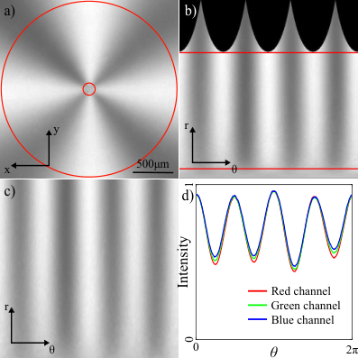
Light generated in different polarisation states produces different intensity patterns measured on the camera (an example for horizontal initial polarisation is shown in Figure 2a)). We calibrate the intensity of our images by recording a background image with the LED off, and two normalisation images with the PSG set to produce horizontal and vertical polarisation respectively. The intensity patterns used for our Fourier analysis are background corrected and normalised to the sum of the two normalisation images. We unwrap the calibrated images from a Cartesian (-) to a polar (-) coordinate frame, relative to the cone centre. The noisy data at the centre and edges of the intensity pattern is removed by selecting a region of interest, delimited by red lines in Figure 2a) and Figure 2b), leaving the cleaned data shown in Figure 2c).
The resulting averaged 1D intensity profile (see Figure 2d)) is , the first row of Equation 11, and from this we obtain the Fourier coefficients C using a fast Fourier transform (FFT) as discussed in section II. Calculation of M requires determination of and , which we achieve following the method outlined in [30, 31]. Systematic errors in these measurements can lead to non-physical Mueller matrices, which can be avoided by converting and into the form shown in Equation (5) of [32] (see Supplement 1). This conversion assumes that there is no loss of polarisation in the beam-splitter and that the Mueller matrix can be parameterised by 3 angles, namely a phase-shift induced between s and p polarisation components, a rotation of the linear polarisation components, and an orientation of the beam-splitter from horizontal. We achieve this normalisation by numerical minimisation of the difference between our measured and normalised matrix while varying all 3 angles. The pseudo-inverse of M is calculated using the singular value decomposition (SVD) method and we finally recover S using Equation 10.
The imperfections of the optical elements, described by the Mueller matrices and , are in general frequency dependent. We identify these matrices for the red, green and blue colour channels of our camera independently. These are applied to the individual intensity patterns for the three colour channels, obtaining S for red, green and blue frequency ranges. Our final white light polarisation state is taken to be their average.
V Results and Discussion
To assess our polarimeter quantitatively, we consider its performance for measurement of the polarised and unpolarised components of the light separately. The polarised component is assessed by measuring the so-called angular accuracy, which can be thought of as the angle between initial and measured polarisation vectors on the Poincaré sphere as demonstrated in Figure 3a). Angular accuracy is defined as
| (12) |
where and . The unpolarised component of the state can be quantified using the degree of polarisation (DOP) accuracy, where the DOP is defined as
| (13) |
and its accuracy is given by the magnitude of the difference between the initial polarisation state DOP and measured DOP. We assess the angular accuracy and DOP accuracy for a range of elliptical and linear initial states. The linear polarisation states are generated by rotating a linear polariser in increments over a range of . Elliptical polarisation states are generated in the same way, with an additional quarter-wave Fresnel rhomb (horizontal fast-axis) after the linear polariser (see Figure 3b) for a Poincaré representation of these polarisation states).
To visualise the angular accuracy only, we set . The remaining Stokes parameters for a range of elliptic input states are shown in Figure 4a), finding excellent agreement between the initial (solid lines) and measured (data points) Stokes parameters. Similar results are obtained for the linear polarisation initial states (not shown). The overall performance can be gauged by taking the average angular accuracy for all elliptical (linear) initial states, which we find to be ().
In addition to the overall angular accuracy of the polarimeter we also investigate its frequency dependence, which is obtained by performing the data analysis on each colour channel of the camera individually. Figure 4b) shows the angular accuracy in the red, green and blue colour bands. We see that the polarimeter has similar performance across the three frequency bands for elliptical (linear) initial states, with average angular accuracies of (), () and () in the red, green and blue colour bands respectively. These results confirm that our polarimeter performs well across the full visible spectrum.

In addition to fully polarised states, our polarimeter also allows measurement of the full Stokes vector. We measure the DOP accuracy for the same elliptical (linear) initial polarisation states as before and calculate the average error to be () across all initial polarisation states and colour channels. Individual colour channel performance is 0.11 (0.10), 0.13 (0.07) and 0.11 (0.08) for the red, green and blue colour channels respectively, showing good performance across the visible spectrum.
The formal equivalence between our polarimeter and the canonical rotating quarter-wave plate polarimeter, enables us to apply the findings of previous optimisation studies. The number of measurements used for Stokes vector determination has been discussed in [33], where it was shown that performance is increased when using more than the minimum required number of measurements. For temporally modulated polarimeters this requires a longer acquisition time, however here we record measurements for many angles simultaneously. In agreement with these studies we find best performance when we use as many values as possible (499). The optimum number of values however changes between anguar accuracy and DOP accuracy measurements. The best angular accuracy results are obtained by averaging all values from 25 pixels to 350 pixels, avoiding the noisy central region. Optimal DOP accuracy results are instead found when averaging over only 10 values at the edge of the image. We attribute this difference in optimal pixel range to the background noise level. At small there are fewer unique values due to pixellation, reducing contrast and increaseing backgroud noise. This effects the DOP measurements through its reliance on , while leaving angular accuracy measurements relatively unafected.
Performance can also be improved by adjusting the retardance, as discussed in [34], with an optimal retardance of . The glass used in our Fresnel cone (BK7) has an average refractive index of for white light, resulting in a retardance of approximately . By engineering the Fresnel cone with refractive index of 1.86 (LaSF9 glass), a retardance of can be achieved, which is predicted to reduce the effect of measurement noise on the polarisation results. Compensation for errors in retardance value and azimuthal misalignment error of the linear polariser have also been discussed in [28] and could be applied to the Fresnel cone polarimeter.
A potential advantage of our Fresnel cone polarimeter compared to conventional polarimeters is the increased acquisition rate. In our camera-based system, the data acquisition rate is set by the frame rate, allowing Stokes measurements in the kHz range using a suitable camera. Using individual detectors, as outlined in section V, this could be increased into the MHz or GHz range. We can make an estimate of the performance of a setup with individual detectors by taking a subset of our camera data. Initial tests taking only 9 equally azimuthally spaced camera pixels (at ) around the cone shows an average angular accuracy of () and average DOP error of () for elliptical (linear) input polarisation states, confirming that the system still performs well even with few measurements.
VI Conclusions
We have demonstrated a full Stokes polarimeter based on the back-reflection from a Fresnel cone, and show that it is the spatial analogue to the ubiquitous rotating quarter-wave plate technique. We characterise the performance of our polarimeter by measuring the angular accuracy, experimentally demonstrating this to have an average of and , with average DOP errors of and for elliptical and linear polarisation states respectively. We have also shown that the polarimeter performs well across the visible spectrum, by measuring the angular accuracy and DOP error in the red, green and blue colour bands respectively. This proof of principle experiment uses off-the-shelf polarisation components, and specialised optics could improve performance while reducing size. Previous research on polarimeter optimisation can also be applied to our polarimeter, improving performance through optimisation of refractive index and measurement strategy.
Not only does our device record a full Stokes vector in a single shot for broadband light, but Fresnel cone polarimeters are robust, stable and low-cost (£500). This new capability could find many uses in a wide range of applications, for example a multi-domain polychromatic spectro-polarimeter [35, 36], which provides Stokes measurements as a function of wavelength. While our polarimeter is not compatible with direct imaging, scanning techniques such as confocal or 2-photon microscopy could be equipped with our Fresnel cone polarimeter, adding polarisation sensitivity to these techniques.
Funding Information
This work has been supported by EPSRC Quantum Technology Program grant number EP/M01326X/1. R. D. Hawley’s work was supported by the EPSRC CDT in Intelligent Sensing and Measurement, Grant Number EP/L016753/1.
Acknowledgments
We would like to thank Gergely Ferenczi and Jonathan Taylor for useful and interesting discussions.
Supplemental Documents
See Supplement 1 for supporting content. A dataset containing the raw data and analysis code can be found at: http://dx.doi.org/10.5525/gla.researchdata.650.
References
- [1] E. Costa, P. Soffitta, R. Bellazzini, A. Brez, N. Lumb, and G. Spandre, Nature 411, 662 (2001), arXiv:0107486 [astro-ph] .
- [2] B. W. Lites, M. Kubo, H. Socas‐Navarro, T. Berger, Z. Frank, R. Shine, T. Tarbell, A. Title, K. Ichimoto, Y. Katsukawa, S. Tsuneta, Y. Suematsu, T. Shimizu, and S. Nagata, The Astrophysical Journal 672, 1237 (2008).
- [3] M. F. Sterzik, S. Bagnulo, and E. Palle, Nature 483, 64 (2012).
- [4] P. M. Johnson, D. A. Olson, S. Pankratz, T. Nguyen, J. Goodby, M. Hird, and C. C. Huang, Physical Review Letters 84, 4870 (2000).
- [5] N. N. Kovaleva, A. V. Boris, C. Bernhard, A. Kulakov, A. Pimenov, A. M. Balbashov, G. Khaliullin, and B. Keimer, Physical Review Letters 93, 147204 (2004).
- [6] M. Losurdo, M. Bergmair, G. Bruno, D. Cattelan, C. Cobet, A. De Martino, K. Fleischer, Z. Dohcevic-Mitrovic, N. Esser, M. Galliet, R. Gajic, D. Hemzal, K. Hingerl, J. Humlicek, R. Ossikovski, Z. V. Popovic, and O. Saxl, Journal of Nanoparticle Research 11, 1521 (2009), arXiv:arXiv:1011.1669v3 .
- [7] S. R. Cloude and E. Pettier, IEEE Transactions on Geoscience and Remote Sensing 34, 498 (1996).
- [8] D. J. Diner, A. Davis, B. Hancock, G. Gutt, R. a. Chipman, and B. Cairns, Applied optics 46, 8428 (2007).
- [9] R. Imazawa, Y. Kawano, T. Ono, and K. Itami, Review of Scientific Instruments 87 (2016), 10.1063/1.4939444.
- [10] D. S. Greenfield, R. W. Knighton, and X. R. Huang, American Journal of Ophthalmology 129, 715 (2000).
- [11] N. Ghosh, Journal of Biomedical Optics 16, 110801 (2011).
- [12] J. Vizet, S. Manhas, J. Tran, P. Validire, A. Benali, E. Garcia-Caurel, A. Pierangelo, A. D. Martino, and D. Pagnoux, Journal of Biomedical Optics 21, 071106 (2016).
- [13] W. S. Bickel and W. M. Bailey, American Journal of Physics 53, 468 (1985).
- [14] G. P. Nordin, J. T. Meier, P. C. Deguzman, and M. W. Jones, Journal of the Optical Society of America A 16, 1168 (1999).
- [15] G. Myhre, W.-L. Hsu, A. Peinado, C. LaCasse, N. Brock, R. A. Chipman, and S. Pau, Optics Express 20, 27393 (2012).
- [16] P. Deng, R. B. Jin, X. Zhao, Y. Cao, and J. Yu, Optik 132, 216 (2017).
- [17] J. Chang, N. Zeng, H. He, Y. He, and H. Ma, Optics Letters 39, 2656 (2014).
- [18] J. P. Balthasar Mueller, K. Leosson, and F. Capasso, Optica 3, 42 (2016).
- [19] I. Estévez, V. Sopo, A. Lizana, A. Turpin, and J. Campos, Opt. Lett. 41, 4566 (2016).
- [20] H. G. Berry, G. Gabrielse, and A. E. Livingston, Applied Optics 16, 3200 (1977).
- [21] J. M. Bueno, Journal of Optics A: Pure and Applied Optics 2, 216 (2000).
- [22] Y. Liu, G. A. Jones, Y. Peng, and T. H. Shen, Journal of Applied Physics 100 (2006), 10.1063/1.2353894.
- [23] O. Arteaga, J. Freudenthal, B. Wang, and B. Kahr, Applied Optics 51, 6805 (2012).
- [24] S. Pelizzari, L. Rovati, and C. D. Angelis, Proc. SPIE 4285 , 235 (2001).
- [25] J. F. Lin and M. Z. Lee, Optics Communications 285, 1669 (2012).
- [26] N. Radwell, R. D. Hawley, J. B. Götte, and S. Franke-Arnold, Nature Communications 7, 10564 (2016).
- [27] V. A. Dlugunovich, V. N. Snopko, and O. V. Tsaryuk, Journal of Optical Technology 68, 269 (2001).
- [28] C. Flueraru, S. Latoui, J. Besse, and P. Legendre, IEEE Transactions on Instrumentation and Measurement 57, 731 (2008).
- [29] M. J. Romerein, J. N. Philippson, R. L. Brooks, and R. C. Shiell, Applied Optics 50, 5382 (2011).
- [30] R. M. A. Azzam and N. M. Bashara, Ellipsometry and polarized light (North-Holland, 1987).
- [31] H. Fujiwara, Spectroscopic ellipsometry: Principles and applications (Wiley-Blackwell, 2007) Chap. Appendix 4: Jones–Mueller Matrix Conversion.
- [32] P. S. Hauge, Journal of the Optical Society of America 68, 1519 (1978).
- [33] J. S. Tyo, Applied Optics 41, 619 (2002).
- [34] D. S. Sabatke, M. R. Descour, E. L. Dereniak, W. C. Sweatt, S. A. Kemme, and G. S. Phipps, Opt. Lett. 25, 802 (2000).
- [35] F. Snik, J. Craven-Jones, M. Escuti, S. Fineschi, D. Harrington, A. De Martino, D. Mawet, J. Riedi, and J. S. Tyo, Proc. SPIE 9099, 90990B (2014).
- [36] F. Snik, G. van Harten, A. S. Alenin, I. J. Vaughn, and J. S. Tyo, Proc. SPIE 9613, 96130G (2015).