$\mathsf{PPP}$ -Completeness with Connections to Cryptography

Katerina Sotiraki ^†^†thanks: email: katesot@mit.edu. The author was partly supported by NSF grants CNS-1350619, CNS-1718161, CNS-1414119 and by the Chateaubriand Fellowship of the Office for Science and Technology of the Embassy of France in the United States. Affiliation: MIT Manolis Zampetakis ^†^†thanks: email: mzampet@mit.edu. The author was supported by NSF grants CCF-1551875, CCF-1617730, CCF-1650733. Affiliation: MIT Giorgos Zirdelis ^†^†thanks: email: zirdelis.g@husky.neu.edu. The author was supported by NSF grants CNS-1314722, CNS-1413964, CNS-1750795. Affiliation: Northeastern University

Abstract

Polynomial Pigeonhole Principle ( $\mathsf{PPP}$ ) is an important subclass of $\mathsf{TFNP}$ with profound connections to the complexity of the fundamental cryptographic primitives: collision-resistant hash functions and one-way permutations. In contrast to most of the other subclasses of $\mathsf{TFNP}$ , no complete problem is known for $\mathsf{PPP}$ . Our work identifies the first $\mathsf{PPP}$ -complete problem without any circuit or Turing Machine given explicitly in the input: $\mathsf{constrained\mathchar 45\relax SIS}$ , and thus we answer a longstanding open question from [Pap94].

$\mathsf{constrained\mathchar 45\relax SIS}$ : a generalized version of the well-known Short Integer Solution problem ( $\mathsf{SIS}$ ) from lattice-based cryptography.

In order to give some intuition behind our reduction for $\mathsf{constrained\mathchar 45\relax SIS}$ , we identify another $\mathsf{PPP}$ -complete problem with a circuit in the input but closely related to lattice problems: $\mathsf{BLICHFELDT}$ .

$\mathsf{BLICHFELDT}$ : the computational problem associated with Blichfeldt’s fundamental theorem in the theory of lattices.

Building on the inherent connection of $\mathsf{PPP}$ with collision-resistant hash functions, we use our completeness result to construct the first natural hash function family that captures the hardness of all collision-resistant hash functions in a worst-case sense, i.e. it is natural and universal in the worst-case. The close resemblance of our hash function family with $\mathsf{SIS}$ , leads us to the first candidate collision-resistant hash function that is both natural and universal in an average-case sense.

Finally, our results enrich our understanding of the connections between $\mathsf{PPP}$ , lattice problems and other concrete cryptographic assumptions, such as the discrete logarithm problem over general groups.

1 Introduction

The fundamental task of Computational Complexity theory is to classify computational problems according to their inherent computational difficulty. This led to the definition of complexity classes such as $\mathsf{NP}$ which contains the decision problems with efficiently verifiable proofs in the “yes” instances. The search analog of the class $\mathsf{NP}$ , called $\mathsf{FNP}$ , is defined as the class of search problems whose decision version is in $\mathsf{NP}$ . The same definition extends to the class $\mathsf{FP}$ , as the search analog of $\mathsf{P}$ . The seminal works of [JPY88, Pap94] considered search problems in $\mathsf{FNP}$ that are total, i.e. their decision version is always affirmative and thus a solution must always exist. This totality property makes the definition of $\mathsf{FNP}$ inadequate to capture the intrinsic complexity of total problems in the appropriate way as it was first shown in [JPY88]. Moreover, there were evidences for the hardness of total search problems e.g. in [HPV89]. Megiddo and Papadimitriou [MP89] defined the class $\boldsymbol{\mathsf{TFNP}}$ that contains the total search problems of $\mathsf{FNP}$ , and Papadimitriou [Pap94] proposed the following classification rule of problems in $\mathsf{TFNP}$ :

Total search problems should be classified in terms of the profound mathematical principles that are invoked to establish their totality.

Along these lines, many subclasses for $\mathsf{TFNP}$ have been defined. Johnson, Papadimitriou and Yannakakis [JPY88] defined the class $\boldsymbol{\mathsf{PLS}}$ . A few years later, Papadimitriou [Pap94] defined the complexity classes $\boldsymbol{\mathsf{PPA}}$ , $\boldsymbol{\mathsf{PPAD}}$ , $\boldsymbol{\mathsf{PPADS}}$ and $\boldsymbol{\mathsf{PPP}}$ , each one associated with a profound mathematical principle in accordance with the above classification rule. More recently, the classes $\boldsymbol{\mathsf{CLS}}$ and $\boldsymbol{\mathsf{PWPP}}$ were defined in [DP11] and [Jer16], respectively. In Section 1.1 we give a high-level description of all these classes.

Finding complete problems for the above classes is important as it enhances our understanding of the underlying mathematical principles. In turn, such completeness results reveal equivalences between total search problems, that seemed impossible to discover without invoking the definition of these classes. Since the definition of these classes in [JPY88, Pap94] it was clear that the completeness results about problems that don’t have explicitly a Turing machine or a circuit as a part of their input are of particular importance. For this reason it has been established to call such problems natural in the context of the complexity of total search problems (see [FRG18]).

Many natural complete problems are known for $\mathsf{PLS}$ and $\mathsf{PPAD}$ , and recently natural complete problems for $\mathsf{PPA}$ were identified too (see Section 1.1). However, no natural complete problems are known for the classes $\mathsf{PPP}$ , $\mathsf{PWPP}$ that have profound connections with the hardness of important cryptographic primitives, as we explain later in detail.

Our Contributions. Our main contribution is to provide the first natural complete problems for $\mathsf{PPP}$ and $\mathsf{PWPP}$ , and thus solve a longstanding open problem from [Pap94]. Beyond that, our $\mathsf{PPP}$ completeness results lead the way towards answering important questions in cryptography and lattice theory as we highlight below.

Universal Collision-Resistant Hash Function. Building on the inherent connection of $\mathsf{PWPP}$ with collision-resistant hash functions, we construct a natural hash function family $\mathcal{H}_{\mathsf{cSIS}}$ with the following properties:

-

Worst-Case Universality. No efficient algorithm can find a collision in every function of the family $\mathcal{H}_{\mathsf{cSIS}}$ , unless worst-case collision-resistant hash functions do not exist.

Moreover, if an (average-case hard) collision-resistant hash function family exists, then there exists an efficiently samplable distribution $\mathcal{D}$ over $\mathcal{H}_{\mathsf{cSIS}}$ , such that $(\mathcal{D},\mathcal{H}_{\mathsf{cSIS}})$ is an (average-case hard) collision-resistant hash function family.
-

Average-Case Hardness. No efficient algorithm can find a collision in a function chosen uniformly at random from $\mathcal{H}_{\mathsf{cSIS}}$ , unless we can efficiently find short lattice vectors in any (worst-case) lattice.

The first property of $\mathcal{H}_{\mathsf{cSIS}}$ is reminiscent of the existence of worst-case one-way functions from the assumption that $\mathsf{P}\neq\mathsf{NP}$ [Sel92]. The corresponding assumption for the existence of worst-case collision-resistance hash functions is assuming $\mathsf{FP}\neq\mathsf{PWPP}$ , but our hash function family $\mathcal{H}_{\mathsf{cSIS}}$ is the first natural definition that does not involve circuits, and admits this strong completeness guarantee in the worst-case.

The construction and properties of $\mathcal{H}_{\mathsf{cSIS}}$ lead us to the first candidate of a natural and universal collision-resistant hash function family. The idea of universal constructions of cryptographic primitives was initiated by Levin in [Lev87], who constructed the first universal one-way function and followed up by [Lev03, KN09]. Using the same ideas we can also construct collision a universal collision-resistant hash function family as we describe in Appendix C. The constructed hash function though invokes in the input an explicit description of a Turing machine and hence it fails to be natural, with the definition of naturality that we described before. In contrast, our candidate construction is natural, simple, and could have practical applications.

Complexity of Lattice Problems in $\mathsf{PPP}$ . The hardness of lattice problems in $\mathsf{NP}\cap\mathsf{coNP}$ [AR04] has served as the foundation for numerous cryptographic constructions in the past two decades. This line of work was initiated by the breakthrough work of Ajtai [Ajt96], and later developed in a long series of works (e.g. [AD97, MR07, Reg09, GPV08, Pei09, GVW13, BLP+13, BV14, GSW13, GVW15b, GKW17, WZ17, PRSD17]). This wide use of search (approximation) lattice problems further motivates their study.

We make progress in understanding this important research front by showing that:

1.

the computational problem $\mathsf{BLICHFELDT}$ associated with Blichfeldt’s theorem, which can be viewed as a generalization of Minkowski’s theorem, is $\mathsf{PPP}$ -complete,
2.

the $\mathsf{cSIS}$ problem, a constrained version of the Short Integer Solution ( $\mathsf{SIS}$ ), is $\mathsf{PPP}$ -complete,
3.

we combine known results and techniques from lattice theory to show that most approximation lattice problems are reducible to $\mathsf{BLICHFELDT}$ and $\mathsf{cSIS}$ .

These results create a new path towards a better understanding of lattice problems in terms of complexity classes.

Complexity of Other Cryptographic Assumptions. Besides lattice problems, we discuss the relationship of other well-studied cryptographic assumptions and $\mathsf{PPP}$ . Additionally, we formulate a white-box variation of the generic group model for the discrete logarithm problem [Sho97]; we observe that this problem is in $\mathsf{PPP}$ and is another natural candidate for being $\mathsf{PPP}$ -complete.

1.1 Related Work

In this section we discuss the previous work on the complexity of total search problems, that has drawn attention from the theoretical computer science community over the past decades. We start with a high-level description of the total complexity classes and then discuss the known results for each one of them.

$\boldsymbol{\mathsf{PLS}}$ .: The class of problems whose totality is established using a potential function argument.
Every finite directed acyclic graph has a sink.
$\boldsymbol{\mathsf{PPA}}$ .: The class of problems whose totality is proved through a parity argument.
Any finite graph has an even number of odd-degree nodes.
$\boldsymbol{\mathsf{PPAD}}$ .: The class of problems whose totality is proved through a directed parity argument.
All directed graphs of degree two or less have an even number of degree one nodes.
$\boldsymbol{\mathsf{PPP}}$ .: The class of problems whose totality is proved through a pigeonhole principle argument.
Any map from a set $S$ to itself either is onto or has a collision.

Using the same spirit two more classes were defined after [Pap94], in [DP11] and [Jer16].

$\boldsymbol{\mathsf{CLS}}$ .: The class of problems whose totality is established using both a potential function argument and a parity argument.
$\boldsymbol{\mathsf{PWPP}}$ .: The class of problems whose totality is proved through a weak pigeonhole principle.
Any map from a set $S$ to a strict subset of $S$ has a collision.

Refer to caption — Figure 1: The classes $\mathsf{PPP}$ and $\mathsf{PWPP}$ in the $\mathsf{TFNP}$ world.

Recently, a syntactic analog $\mathsf{PTFNP}$ of the semantic class $\mathsf{TFNP}$ has been defined in [GP17], and a complete problem for this class has been identified. It has also been shown that all the classes we described above are subsets of $\mathsf{PTFNP}$ . Oracle separations between all these classes are known [BCE+98], with the only exception of whether $\mathsf{PLS}$ is contained in $\mathsf{PPAD}$ .

$\boldsymbol{\mathsf{PLS}}$ -completeness. The class $\mathsf{PLS}$ represents the complexity of local optimization problems. Some important problems that have been shown to be $\mathsf{PLS}$ -complete are: Local Max-Cut [SY91], Local Travelling Salesman Problem [Pap92], and Finding a Pure Nash Equilibrium [FPT04]. Recently, important results for the smoothed complexity of the Local Max-Cut problem were shown in [ER17, ABPW17].

$\boldsymbol{\mathsf{PPAD}}$ -completeness. Arguably, the most celebrated application of the complexity of total search problems is the characterization of the computational complexity of finding a Nash equilibrium in terms of $\mathsf{PPAD}$ -completeness [DGP09, CDT09]. This problem lies in the heart of game theory and economics. The proof that Nash Equilibrium is $\mathsf{PPAD}$ -complete initiated a long line of research in the intersection of computer science and game theory and revealed connections between the two scientific communities that were unknown before (e.g. [EGG06, CDDT09, VY11, KPR+13, CDO15, Rub15, Rub16, CPY17, SSB17]).

$\boldsymbol{\mathsf{PPA}}$ -completeness. $\mathsf{PPA}$ -complete problems usually arise as the undirected generalizations of their $\mathsf{PPAD}$ -complete analogs. For example, Papadimitriou [Pap94] showed that Sperner’s Lemma in a 3-D cube is $\mathsf{PPAD}$ -complete and later Grigni [Gri01] showed that Sperner’s Lemma in a 3-manifold consisting of the product of a Möbius strip and a line segment is $\mathsf{PPA}$ -complete. Since Möbius strip is non-orientable, this indeed is a non-directed version of the Sperner’s Lemma. Similarly, other problems have been showed to be $\mathsf{PPA}$ -complete, all involving some circuit as an input in their definition [ABB15, DEF+16, BIQ+17]. Recently, the first natural $\mathsf{PPA}$ -complete problem, without a circuit as part of the input, has been identified in [FRG18]. This illustrates an interesting relation between $\mathsf{PPA}$ and complexity of social choice theory problems.

$\boldsymbol{\mathsf{CLS}}$ -completeness. The $\mathsf{CLS}$ class was defined in [DP11] to capture the complexity of problems such as P-matrix LCP, computing KKT-points, and finding Nash equilibria in congestion and network coordination games. Recently, it has been proved that the problem of finding a fixed point whose existence invokes Banach’s Fixed Point Theorem, is $\mathsf{CLS}$ -complete [DTZ18, FGMS17].

$\boldsymbol{\mathsf{TFNP}}$ and cryptography. The connection of $\mathsf{TFNP}$ and cryptography was illustrated by Papadimitriou in [Pap94], where he proved that if $\mathsf{PPP}=\mathsf{FP}$ then one-way permutations cannot exist. In [BO06], a special case of integer factorization was shown to be in $\mathsf{PPA}\cap\mathsf{PPP}$ . This was generalized in [Jer16] by proving that the problem of factoring integers is in $\mathsf{PPA}\cap\mathsf{PPP}$ under randomized reductions. Recently, strong cryptographic assumptions were used to prove the average-case hardness of $\mathsf{PPAD}$ and $\mathsf{CLS}$ [BPR15, GPS16, HY17]. In [RSS17] it was shown that average-case $\mathsf{PPAD}$ hardness does not imply one-way function under black-box reductions, whereas in [HNY17] it was shown that any hard on average problem in $\mathsf{NP}$ implies the average case hardness of $\mathsf{TFNP}$ . Finally, in [KNY17] it is proved that the existence of multi-collision resistant hash functions is equivalent with a variation of the total search problem $\mathsf{RAMSEY}$ , which is not known to belong to any of the above complexity classes. Interestingly, they prove that a variation of $\mathsf{RAMSEY}$ called colorful-Ramsey ( $\mathsf{C\mathchar 45\relax RAMSEY}$ ) is $\mathsf{PWPP}$ -hard. Although this an important result, the problem $\mathsf{C\mathchar 45\relax RAMSEY}$ still invokes a circuit in the input and in not known to be in $\mathsf{PWPP}$ , hence does not resolve the problem of identifying a natural complete problem for $\mathsf{PWPP}$ .

$\boldsymbol{\mathsf{TFNP}}$ and lattices. In [BJP+15] it was shown that the computational analog of Minkowski’s theorem (namely $\mathsf{MINKOWSKI}$ ) is in $\mathsf{PPP}$ , was conjectured that it is also $\mathsf{PPP}$ -complete. The authors justified their conjecture by showing that $\mathsf{EQUAL\mathchar 45\relax SUMS}$ , a problem from [Pap94] that is conjectured to be $\mathsf{PPP}$ -complete, reduces to $\mathsf{MINKOWSKI}$ . Additionally, they show that a number theoretic problem called $\mathsf{DIRICHLET}$ reduces to $\mathsf{MINKOWSKI}$ , and thus is in $\mathsf{PPP}$ . In [HRRY17] it is proven that the problem $\mathsf{NUMBER\mathchar 45\relax BALANCING}$ is equivalent to a polynomial approximation of Minkowski’s theorem in the $\ell_{2}$ norm (via Cook reductions for both directions).

1.2 Roadmap of the paper

We start our exposition with a brief description of the results contained in this paper. First we briefly describe the $\mathsf{PPP}$ -completeness of $\mathsf{BLICHFELDT}$ that illustrates some of the basic ideas behind our main result that $\mathsf{cSIS}$ is $\mathsf{PPP}$ -complete. The complete proof of the $\mathsf{PPP}$ -completeness of $\mathsf{BLICHFELDT}$ can be found in Section 3. We suggest to readers that have experience with the fundamental concepts of the theory of lattices to skip the details Section 3.

Then, we present a brief description of our main theorem and its proof. The complete proof of the $\mathsf{PPP}$ -completeness of $\mathsf{cSIS}$ can be found in Section 4.

In Section 5 we describe the $\mathsf{PPP}$ -completeness of a weaker version of $\mathsf{cSIS}$ and its relation with the definition of the first natural universal collision resistant hash function family in the worst-case sense. This proof also provides the first candidate for a collision resistant hash function family that is both natural and universal in the average-case sense.

Finally in Section 6 we present, for completeness of our exposition, other lattice problems that are already known to belong to $\mathsf{PPP}$ and $\mathsf{PWPP}$ and in Section 7 we present more general other cryptographic assumptions that belong to $\mathsf{PPP}$ and $\mathsf{PWPP}$ .

1.3 Overview of the Results

Before we describe our results in more detail we define the class $\mathsf{PPP}$ more formally. The class $\mathsf{PPP}$ contains the set of problems that are reducible to the $\mathsf{PIGEONHOLE\penalty\ CIRCUIT}$ problem. The input to $\mathsf{PIGEONHOLE\penalty\ CIRCUIT}$ is a binary circuit $\mathcal{C}:\{0,1\}^{n}\to\{0,1\}^{n}$ and its output is either an $\boldsymbol{\underaccent{\bar}{x}}\in\{0,1\}^{n}$ such that $\mathcal{C}(\boldsymbol{\underaccent{\bar}{x}})=\boldsymbol{\underaccent{\bar}{0}}$ , or a pair $\boldsymbol{\underaccent{\bar}{x}},\boldsymbol{\underaccent{\bar}{y}}\in\{0,1\}^{n}$ such that $\boldsymbol{\underaccent{\bar}{x}}\neq\boldsymbol{\underaccent{\bar}{y}}$ and $\mathcal{C}(\boldsymbol{\underaccent{\bar}{x}})=\mathcal{C}(\boldsymbol{\underaccent{\bar}{y}})$ .

Our first and technically most challenging result is to identify and prove the $\mathsf{PPP}$ -completeness of two problems, both of which share similarities with lattice problems. For our exposition, a lattice $\mathcal{L}\subseteq\mathbb{Z}^{n}$ can be viewed as a finitely generated additive subgroup of $\mathbb{Z}^{n}$ . A lattice $\mathcal{L}=\mathcal{L}(\mathbf{B}):=\mathbf{B}\cdot\mathbb{Z}^{n}$ is generated by a full-rank matrix $\mathbf{B}\in\mathbb{Z}^{n\times n}$ , called basis. In the rest of this section we also use the fundamental parallelepiped of $\mathcal{L}$ defined as $\mathcal{P}(\mathcal{L}):=\mathbf{B}\cdot[0,1)^{n}$ .

1.3.1 $\boldsymbol{\mathsf{BLICHFELDT}}$ is $\boldsymbol{\mathsf{PPP}}$ -complete.

We define the $\mathsf{BLICHFELDT}$ problem as the computational analog of Blichfeldt’s theorem (see Theorem 3.1). Its input is a basis for a lattice $\mathcal{L}\subseteq\mathbb{Z}^{n}$ and a set $S\subseteq\mathbb{Z}^{n}$ of cardinality greater or equal to the volume of $\mathcal{P}(\mathcal{L})$ . Its output is either a point in $S$ that belongs to $\mathcal{L}$ , or for two (different) points in $S$ such that their difference belongs to $\mathcal{L}$ . In the overview below, we explain why such an output always exists. Notice that finding a solution to $\mathsf{BLICHFELDT}$ becomes trivial if the input representation of $S$ has length proportional to its size, i.e. one can iterate over all element pairs of $S$ . The problem becomes challenging when $S$ is represented succinctly. We introduce a notion for a succinct representation of sets that we call value function. Informally, a value function for a set $S$ is a small circuit that takes as input $\lceil\log(|S|)\rceil$ bits that describe an index $i\in\{0,\ldots,|S|-1\}$ , and outputs $\mathbf{s}_{i}\in S$ .

We give a proof overview of our first main theorem, and highlight the obstacles that arise, along with our solutions.

Theorem 3.5.

The $\mathsf{BLICHFELDT}$ problem is $\mathsf{PPP}$ -complete.

$\mathsf{PPP}$ Membership of $\mathsf{BLICHFELDT}$ Overview. We denote with $[n]$ the set $\{0,\ldots,n-1\}$ . We define the map $\boldsymbol{\sigma}:\mathbb{Z}^{n}\rightarrow\mathcal{P}(\mathcal{L})\cap\mathbb{Z}^{n}$ that reduces any point in $\mathbb{Z}^{n}$ modulo the parallelepiped to $\mathcal{P}(\mathcal{L})\cap\mathbb{Z}^{n}$ , i.e. $\penalty\ (\bmod\penalty\ \mathcal{P}(\mathcal{L}))$ . Using $\boldsymbol{\sigma}$ we can efficiently check the membership of any $\mathbf{v}\in\mathbb{Z}^{n}$ in $\mathcal{L}$ , by checking if $\boldsymbol{\sigma}$ maps $\mathbf{v}$ to the origin. Observe that if $\boldsymbol{\sigma}(\mathbf{x})=\boldsymbol{\sigma}(\mathbf{y})$ then $\mathbf{x}-\mathbf{y}\in\mathcal{L}$ .

We show in Lemma 3.2 that $\vol(\mathcal{P}(\mathcal{L}))=|\mathcal{P}(\mathcal{L})\cap\mathbb{Z}^{n}|$ , hence the input requirement for $S$ is equivalent to $|S|\geq|\mathcal{P}(\mathcal{L})\cap\mathbb{Z}^{n}|$ . Notice that the points of $S$ after applying the map $\boldsymbol{\sigma}$ , either have a collision in $\mathcal{P}(\mathcal{L})\cap\mathbb{Z}^{n}$ or a preimage of the origin exists in $S$ . It follows by a pigeonhole argument that a solution to $\mathsf{BLICHFELDT}$ always exists. For the rest of this part we assume that $|S|=|\mathcal{P}(\mathcal{L})\cap\mathbb{Z}^{n}|$ and let $n=\lceil\log(|S|)\rceil$ .

We construct a circuit $\mathcal{C}:\{0,1\}^{n}\to\{0,1\}^{n}$ that on input an appropriate index $i$ , evaluates the value function of $S$ to obtain $\mathbf{s}_{i}\in S$ , and computes $\boldsymbol{\sigma}(\mathbf{s}_{i})$ . The most challenging part of the proof is to construct an efficient map from $\boldsymbol{\sigma}(S)$ to $[|\mathcal{P}(\mathcal{L})\cap\mathbb{Z}^{n}|]$ in the following way. We define an appropriate parallelepiped $D=[L_{1}]\times[L_{2}]\times\dots\times[L_{n}]$ where the $L_{i}$ are non-negative integers, and a bijection $\boldsymbol{\pi}:\mathcal{P}(\mathcal{L})\cap\mathbb{Z}^{n}\rightarrow D$ . Because $D$ is a cartesian product, a natural efficient indexing procedure exists as described in Lemma 2.1. This allows to map $\boldsymbol{\pi}(\boldsymbol{\sigma}(\mathbf{s}_{i}))$ to $j\in[|\mathcal{P}(\mathcal{L})\cap\mathbb{Z}^{n}|]$ . The circuit $\mathcal{C}$ outputs the binary decomposition of $j$ . It follows that any $\boldsymbol{\underaccent{\bar}{x}}$ such that $\mathcal{C}(\boldsymbol{\underaccent{\bar}{x}})=\boldsymbol{\underaccent{\bar}{0}}$ corresponds to a vector $\mathbf{x}\in S$ such that $\boldsymbol{\sigma}(\mathbf{x})=\mathbf{0}$ . On the other hand, a collision $\mathcal{C}(\boldsymbol{\underaccent{\bar}{x}})=\mathcal{C}(\boldsymbol{\underaccent{\bar}{y}})$ with $\boldsymbol{\underaccent{\bar}{x}}\neq\boldsymbol{\underaccent{\bar}{y}}$ corresponds to a collision $\boldsymbol{\sigma}_{S}(\mathbf{x})=\boldsymbol{\sigma}_{S}(\mathbf{y})$ , where $\boldsymbol{\sigma}_{S}$ is the restriction of $\boldsymbol{\sigma}$ on $S$ , and hence $\mathbf{x}-\mathbf{y}\in\mathcal{L}$ .

$\mathsf{PPP}$ Hardness of $\mathsf{BLICHFELDT}$ Overview. We start with a circuit $\mathcal{C}:\{0,1\}^{n}\rightarrow\{0,1\}^{n}$ that is an input to $\mathsf{PIGEONHOLE\penalty\ CIRCUIT}$ . We construct a set $S$ and a lattice $\mathcal{L}$ as input to $\mathsf{BLICHFELDT}$ in the following way. The set $S$ contains the elements $\mathbf{s}_{\boldsymbol{\underaccent{\bar}{x}}}=\begin{bmatrix}\boldsymbol{\underaccent{\bar}{x}}\\ \mathcal{C}(\boldsymbol{\underaccent{\bar}{x}})\end{bmatrix}\in\{0,1\}^{2n}$ and is represented succinctly with the value function that maps $\boldsymbol{\underaccent{\bar}{x}}$ to $\mathbf{s}_{\boldsymbol{\underaccent{\bar}{x}}}$ . Notice that $|S|=2^{n}$ . The lattice $\mathcal{L}$ consists of all $\boldsymbol{\underaccent{\bar}{v}}\in\{0,1\}^{2n}$ that satisfy the equation $[\boldsymbol{0}_{n}\penalty\ \penalty\ \mathbf{I}_{n}]\cdot\boldsymbol{\underaccent{\bar}{v}}=\boldsymbol{0}\penalty\ (\bmod\penalty\ 2)$ . By Lemma 2.3, one can efficiently obtain a basis from this description of $\mathcal{L}$ and in addition the volume of $\mathcal{P}(\mathcal{L})$ is at most $2^{n}$ . Thus, $S$ and $\mathcal{L}$ is a valid input for $\mathsf{BLICHFELDT}$ .

The output of $\mathsf{BLICHFELDT}$ is either an $\mathbf{s}_{\boldsymbol{\underaccent{\bar}{x}}}=\begin{bmatrix}\boldsymbol{\underaccent{\bar}{x}}\\ \mathcal{C}(\boldsymbol{\underaccent{\bar}{x}})\end{bmatrix}\in S\cap\mathcal{L}$ that (by construction of $\mathcal{L}$ ) implies $\mathcal{C}(\boldsymbol{\underaccent{\bar}{x}})=\mathbf{0}$ , or two different elements of $S$ , $\mathbf{s}_{\boldsymbol{\underaccent{\bar}{x}}}=\begin{bmatrix}\boldsymbol{\underaccent{\bar}{x}}\\ \mathcal{C}(\boldsymbol{\underaccent{\bar}{x}})\end{bmatrix}$ , $\mathbf{s}_{\boldsymbol{\underaccent{\bar}{y}}}=\begin{bmatrix}\boldsymbol{\underaccent{\bar}{y}}\\ \mathcal{C}(\boldsymbol{\underaccent{\bar}{y}})\end{bmatrix}$ with $\mathbf{s}_{\boldsymbol{\underaccent{\bar}{x}}}-\mathbf{s}_{\boldsymbol{\underaccent{\bar}{y}}}\in\mathcal{L}$ that implies $\boldsymbol{\underaccent{\bar}{x}}\neq\boldsymbol{\underaccent{\bar}{y}}$ and (by construction of $\mathcal{L}$ ) $\mathcal{C}(\boldsymbol{\underaccent{\bar}{x}})=\mathcal{C}(\boldsymbol{\underaccent{\bar}{y}})$ .

1.3.2 $\boldsymbol{\mathsf{cSIS}}$ is $\boldsymbol{\mathsf{PPP}}$ -complete.

Part of the input to $\mathsf{BLICHFELDT}$ is represented with a value function which requires a small circuit. As we explained before this makes $\mathsf{BLICHFELDT}$ a non-natural problem with the respect to the definition of naturality in the context of the complexity of total search problems. We now introduce a natural problem that we call constrained Short Integer Solution ( $\mathsf{cSIS}$ ), and show that it is $\mathsf{PPP}$ -complete. The $\mathsf{cSIS}$ problem is a generalization of the well-known Short Integer Solution ( $\mathsf{SIS}$ ) problem, and discuss their connection in Section 5.2.

The input is $\mathbf{A}\in\mathbb{Z}_{q}^{n\times m}$ , $\mathbf{G}\in\mathbb{Z}_{q}^{d\times m}$ and $\mathbf{b}\in\mathbb{Z}_{q}^{d}$ , for some positive integer $q$ and $m\geq(n+d)\lceil\log(q)\rceil$ . The matrix $\mathbf{G}$ has the property that for every $\mathbf{b}$ we can efficiently find an $\mathbf{x}\in\{0,1\}^{m}$ such that $\mathbf{G}\mathbf{x}=\mathbf{b}\penalty\ (\bmod\penalty\ q)$ . We define such matrices as binary invertible. The output is either a vector $\mathbf{x}\in\{0,1\}^{m}$ such that $\mathbf{A}\mathbf{x}=\mathbf{0}\penalty\ (\bmod\penalty\ q)$ and $\mathbf{G}\mathbf{x}=\mathbf{b}\penalty\ (\bmod\penalty\ q)$ , or two different vectors $\mathbf{x},\mathbf{y}\in\{0,1\}^{m}$ such that $\mathbf{A}(\mathbf{x}-\mathbf{y})=\mathbf{0}\penalty\ (\bmod\penalty\ q)$ and $\mathbf{G}\mathbf{x}=\mathbf{G}\mathbf{y}=\mathbf{b}\penalty\ (\bmod\penalty\ q)$ . We give a proof overview of the next theorem, and a full proof in Section 4.

Theorem 4.11.

The $\mathsf{cSIS}$ problem is $\mathsf{PPP}$ -complete.

$\mathsf{PPP}$ Membership of $\mathsf{cSIS}$ Overview. We show the membership of $\mathsf{cSIS}$ in $\mathsf{PPP}$ for the general class of binary invertible matrices $\mathbf{G}$ in Section 4. In order to simplify the exposition, we assume that $q=2^{\ell}$ and $\mathbf{G}$ to be the “gadget” matrix concatenated with a random matrix $\mathbf{V}$ . That is, $\mathbf{G}$ has the form $\left[\mathbf{I}_{d}\otimes\boldsymbol{\gamma}^{T}\,\,\,\mathbf{V}\right]$ where $\boldsymbol{\gamma}^{T}=[1,2,\ldots,2^{\ell}]$ .

Let $\mathbf{A}\in\mathbb{Z}_{q}^{n\times m}$ , $\mathbf{G}\in\mathbb{Z}_{q}^{d\times m}$ , and $\mathbf{b}\in\mathbb{Z}_{q}^{d}$ be the input to $\mathsf{cSIS}$ . We now explain why $m\geq(n+d)\ell$ suffices to always guarantee a solution to $\mathsf{cSIS}$ . First, observe that the first $\ell\cdot d$ columns of $\mathbf{G}$ , corresponding to the gadget matrix $[\mathbf{I}_{d}\otimes\boldsymbol{\gamma}^{T}]$ , are enough to guarantee that for every $\mathbf{r}^{\prime}\in\mathbb{Z}_{q}^{m-\ell d}$ there exists an $\mathbf{r}$ such that $\mathbf{G}\begin{bmatrix}\mathbf{r}\\ \mathbf{r}^{\prime}\end{bmatrix}=\mathbf{b}\penalty\ (\bmod\penalty\ q)$ . Hence, there are at least $q^{m-\ell d}$ solutions to the equation $\mathbf{G}\mathbf{x}=\mathbf{b}\penalty\ (\bmod\penalty\ q)$ . Also, there are $2^{\ell n}$ possible values for $\mathbf{A}\mathbf{x}\penalty\ (\bmod\penalty\ q)$ . By a pigeonhole argument a solution to $\mathsf{cSIS}$ always exists. To complete the membership proof, issues similar to $\mathsf{BLICHFELDT}$ with the circuit representation of the problem instance appear, but we overcome them using similar ideas.

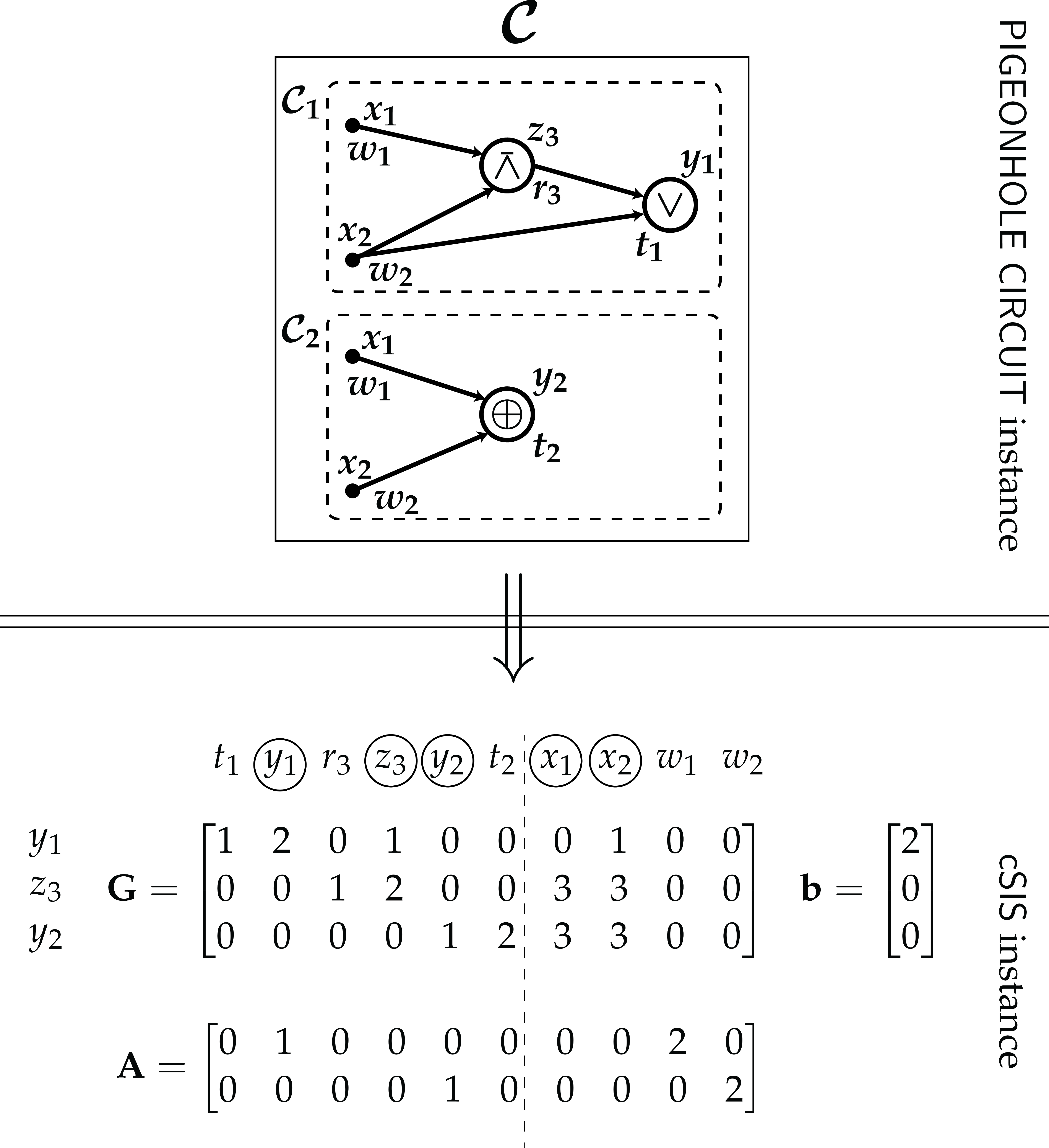
$\mathsf{PPP}$ Hardness of $\mathsf{cSIS}$ Overview. We start with a circuit $\mathcal{C}:\{0,1\}^{n}\rightarrow\{0,1\}^{n}$ that is an input to $\mathsf{PIGEONHOLE\penalty\ CIRCUIT}$ . Since the input of $\mathsf{PIGEONHOLE\penalty\ CIRCUIT}$ is a circuit and the input of $\mathsf{cSIS}$ is a pair of matrices and a vector, we need to represent this circuit in an algebraic way. In particular, we device a way to encode the circuit in a binary invertible matrix $\mathbf{G}$ and a vector $\mathbf{b}$ . To gain a better intuition of why this is possible, we note that a $\mathsf{NAND}$ gate $x\penalty\ \bar{\wedge}\penalty\ y=z$ can be expressed as the linear modular equation $x+y+2z-w=2\penalty\ (\bmod\penalty\ 4)$ , where $x,y,z,w\in\{0,1\}$ . By a very careful construction, we can encode these linear modular equations in a binary invertible matrix $\mathbf{G}$ . For further details we defer to Section 4.

Since $\mathsf{cSIS}$ with $q=4$ returns a vector such that $\mathbf{A}\mathbf{x}=\boldsymbol{0}\penalty\ (\bmod\penalty\ 4)$ and $\mathsf{PIGEONHOLE\penalty\ CIRCUIT}$ asks for a binary vector such that $\mathcal{\boldsymbol{\underaccent{\bar}{x}}}=\boldsymbol{\underaccent{\bar}{0}}$ , a natural idea is to let $\mathbf{A}$ be of the form $\left[\boldsymbol{0}\,\,\,\mathbf{I}_{n}\right]$ , where the identity matrix corresponds to the columns representing the output of circuit $\mathcal{C}$ in $\mathbf{G}$ . Finally, we argue that a solution to $\mathsf{cSIS}$ with input $\mathbf{A},\mathbf{G}$ and $\mathbf{b}$ as constructed above, gives either a collision or a preimage of zero for the circuit $\mathcal{C}$ as required.

It can be argued that this reduction shares common ideas with the reduction of $3\mathchar 45\relax\mathsf{SAT}$ to $\mathsf{SUBSET\mathchar 45\relax SUM}$ ; this shows the importance of the input conditions for $\mathsf{cSIS}$ and hints to the numerous complications that arise in the proof. Without these conditions, we could end up with a trivial reduction to an $\mathsf{NP}$ -hard problem! Fortunately, we are able to show that our construction satisfies the input conditions of $\mathsf{cSIS}$ .

1.3.3 Towards a Natural and Universal Collision-Resistant Rash Family.

$\mathsf{PWPP}$ is a subclass of $\mathsf{PPP}$ in which a collision always exists; it is not hard to show that variations of both $\mathsf{BLICHFELDT}$ and $\mathsf{cSIS}$ are $\mathsf{PWPP}$ -complete. We tweak the parameters of valid inputs in order to guarantee that a collision always exists. The $\mathsf{PWPP}$ -complete variation of $\mathsf{cSIS}$ , which we denote by $\mathsf{weak\mathchar 45\relax cSIS}$ , gives a function family which is a universal collision-resistant hash function family in a worst-case sense: if there is a function family that contains at least one function for which it is hard to find collisions, then our function family also includes a function for which it is hard to find collisions.

We now describe the differences of $\mathsf{cSIS}$ and $\mathsf{weak\mathchar 45\relax cSIS}$ . As before we assume that $q=2^{\ell}$ . The input to $\mathsf{weak\mathchar 45\relax cSIS}$ is a matrix $\mathbf{A}\in\mathbb{Z}_{q}^{n\times m}$ , and a binary invertible matrix $\mathbf{G}\in\mathbb{Z}_{q}^{d\times m}$ . Notice that there is no vector $\mathbf{b}$ in the input, and the relation between $n,m,d$ and $\ell$ is that $m$ has to be strictly greater that $\ell(n+d)$ . Namely, $m>\ell(n+d)$ . This change in the relation of the parameters might seem insignificant, but is actually very important, as it allows us to replace $\mathbf{b}$ in $\mathsf{cSIS}$ by the zero vector. This transforms $\mathsf{weak\mathchar 45\relax cSIS}$ into a pure lattice problem: on input matrices $\mathbf{A},\mathbf{G}$ with corresponding bases $\mathbf{B}_{\mathbf{A}}$ and $\mathbf{B}_{\mathbf{G}}$ , where $\mathbf{G}$ is binary invertible, find two vectors $\mathbf{x}$ and $\mathbf{y}$ such that $\mathbf{x},\mathbf{y}\in\mathcal{L}(\mathbf{B}_{\mathbf{G}})$ and $\mathbf{x}-\mathbf{y}\in\mathcal{L}(\mathbf{B}_{\mathbf{A}})$ .

The great resemblance of $\mathsf{weak\mathchar 45\relax cSIS}$ with $\mathsf{SIS}$ and its completeness for $\mathsf{PWPP}$ lead us to the first candidate for a universal collision-resistant hash function $\mathcal{H}_{\mathsf{cSIS}}=\{h_{\boldsymbol{\underaccent{\bar}{s}}}:\{0,1\}^{k}\rightarrow\{0,1\}^{k^{\prime}}\}$ :

-

The key $\boldsymbol{\underaccent{\bar}{s}}$ is a pair of matrices $(\mathbf{A},\mathbf{G})$ , where $\mathbf{G}$ is binary invertible.
-

Given a key $\boldsymbol{\underaccent{\bar}{s}}=(\mathbf{A},\mathbf{G})$ and a binary vector $\boldsymbol{\underaccent{\bar}{x}}\in\{0,1\}^{k}$ , $h_{\boldsymbol{\underaccent{\bar}{s}}}(\boldsymbol{\underaccent{\bar}{x}})$ is the binary decomposition of $\mathbf{A}\mathbf{u}\penalty\ (\bmod\penalty\ q)$ , where $\mathbf{u}=\begin{bmatrix}\mathbf{r}\\ \boldsymbol{\underaccent{\bar}{x}}\end{bmatrix}$ such that $\mathbf{G}\mathbf{u}=\boldsymbol{0}\penalty\ (\bmod\penalty\ q)$ .

Because lattice problems have worst-to-average case reductions and our hash family is based on a lattice problem, this gives hope for showing that our construction is universal in the average-case sense.

1.3.4 Other Lattice Problems Known to be in $\boldsymbol{\mathsf{PPP}}$ .

We show that the computational analog of Minkowski’s theorem, namely $\mathsf{MINKOWSKI}$ , is in $\mathsf{PPP}$ via a Karp-reduction to $\mathsf{BLICHFELDT}$ . We note that a Karp-reduction showing $\mathsf{MINKOWSKI}\in\mathsf{PPP}$ was shown in [BJP+15]. Based on these two problems and the known reductions between lattice problems, we conclude that a variety of lattice (approximation) problems belong to $\mathsf{PPP}$ ; the most important among them are $n\mathchar 45\relax\mathsf{SVP}$ , $\tilde{O}(n)$ - $\mathsf{SIVP}$ and $n^{2.5}\mathchar 45\relax\mathsf{CVP}$ (see Figure 2).

1.3.5 Other Cryptographic Assumptions in $\boldsymbol{\mathsf{PPP}}$ .

By the definition, the class $\mathsf{PWPP}$ contains all cryptographic assumptions that imply collision-resistant hash functions. These include the factoring of Blum integers, the Discrete Logarithm problem over $\mathbb{Z}_{p}^{*}$ and over elliptic curves, and the $\mathsf{SIS}$ lattice problem (a special case of $\mathsf{weak\mathchar 45\relax cSIS}$ ). Also, Jeřábek [Jer16] showed that the problem of factoring integers is in $\mathsf{PWPP}$ .

We extend the connection between $\mathsf{PPP}$ and cryptography by introducing a white-box model to describe general groups, which we define to be cyclic groups with a succinct representation of their elements and group operation (i.e. a small circuit). We show that the Discrete Logarithm over general groups is in $\mathsf{PPP}$ . An example of a general group is $\mathbb{Z}_{q}^{*}$ . These connections are also summarized in Figure 2.

1.4 Open questions.

Numerous new questions arise from our work and the connections we draw between $\mathsf{PPP}$ , cryptography and lattices. We summarize here some of them.

Open Problem 1.1.

Is there a worst-to-average case reduction from $\mathsf{weak\mathchar 45\relax cSIS}$ to itself?
This result will provide the first natural, in the sense that does not invoke explicitly a Turing machine in the input, and universal collision resistant hash function family.

Open Problem 1.2.

Is $\mathsf{SIS}$ or $\mathsf{MINKOWSKI}$ $\mathsf{PPP}$ -hard?

Open Problem 1.3.

Is $\gamma$ - $\mathsf{SVP}$ in $\mathsf{PPP}$ for $\gamma=o(n)$ ?

Open Problem 1.4.

Is $\gamma$ - $\mathsf{CVP}$ $\mathsf{PPP}$ -hard for $\gamma=\Omega(\sqrt{n})$ ?

Open Problem 1.5.

Is the discrete logarithm problem in $\mathsf{PPP}$ for general elliptic curves?

2 Preliminaries

General Notation. Let $[m]$ be the set $\{0,\dots,m-1\}$ , $\mathbb{N}=\{0,1,2,\dots\}$ and $\mathbb{Z}_{+}=\{1,2,3,\dots\}$ We use small bold letters $\boldsymbol{x}$ to refer to real vectors in finite dimension $\mathbb{R}^{d}$ and capital bold letters $\mathbf{A}$ to refer to matrices in $\mathbb{R}^{d\times\ell}$ . For a matrix $\mathbf{A}$ , we denote by $\mathbf{a}^{T}_{i}$ its $i$ -th row and by $a_{i,j}$ its $(i,j)$ -th element. Let $\mathbf{I}_{n}$ denote the $n$ -dimensional identity matrix. We denote with $\mathbf{E}_{i,j}$ the matrix that has all zeros except that $e_{i,j}=1$ . A function $\negl(k)$ is negligible if $\negl(k)<1/k^{c}$ for any constant $c>0$ and sufficiently large $k$ . All logarithms $\log(\cdot)$ are in base 2.

Vector Norms. We define the $\ell_{p}$ -norm of $\boldsymbol{x}\in\mathbb{R}^{d}$ to be $\lVert\boldsymbol{x}\rVert_{p}=\left(\sum_{i}x_{i}^{p}\right)^{1/p}$ and the $\ell_{\infty}$ -norm of $\boldsymbol{x}$ to be $\lVert\boldsymbol{x}\rVert_{\infty}=\max_{i}\lvert x_{i}\rvert$ . For simplicity we use $\lVert\cdot\rVert$ for the $\ell_{2}$ -norm instead of $\lVert\cdot\rVert_{2}$ . It is well known that $\lVert\boldsymbol{x}\rVert_{p}\leq n^{1/p-1/q}\lVert\boldsymbol{x}\rVert_{q}$ for $p\leq q$ and $\lVert\boldsymbol{x}\rVert_{p}\leq\lVert\boldsymbol{x}\rVert_{q}$ for $p>q$ .

2.1 Complexity Classes and Reductions

Binary Strings and Natural Numbers. We use bold and underlined small letters to refer to binary strings. Binary strings $\boldsymbol{\underaccent{\bar}{x}}\in\{0,1\}^{k}$ of length $k$ can also be viewed as vectors in $\mathbb{Z}^{k}$ . Every binary string $\boldsymbol{\underaccent{\bar}{x}}\in\{0,1\}^{k}$ can be mapped to a non negative integer number through the nonlinear map $\mathsf{bc}:\{0,1\}^{*}\to\mathbb{Z}_{+}$ called bit composition, where $\mathsf{bc}(\boldsymbol{\underaccent{\bar}{x}})=\sum_{i=0}^{k-1}\underaccent{\bar}{x}_{k-i}2^{i}$ . It is trivial to see that actually $\mathsf{bc}$ is a bijective mapping and hence we can define the inverse mapping $\mathsf{bd}:\mathbb{Z}_{+}\to\{0,1\}^{*}$ called bit decomposition, which is also trivial to compute for any given number $m\in\mathbb{Z}_{+}$ .

The bit decomposition function $\mathsf{bd}$ is extended to integer vectors and the result is the concatenation of the bit decomposition of each coordinate of the vector. Similarly, this is also extended to integer matrices. Then of course the bit composition function $\mathsf{bc}$ is no longer well defined because its output can be either a number or a vector of numbers, but for simplicity we still use the notation $\mathsf{bc}$ and it will be made clear from the context whether the output is a number or a vector of numbers. When $\mathsf{bd}$ is applied to a set $\{m_{1},\dots,m_{k}\}$ the output is still a set with the bit decomposition of each element $\{\mathsf{bd}(m_{1}),\dots,\mathsf{bd}(m_{k})\}$ .

Boolean Circuits. A boolean circuit $\mathcal{C}$ with $n$ inputs and $1$ output is represented as a labeled directed acyclic graph with in-degree at most $2$ , with exactly $n$ source nodes and exactly $1$ sink node. Each source node is an input of $\mathcal{C}$ and the sink node is the output of $\mathcal{C}$ . Each of the input nodes of $\mathcal{C}$ is labeled with a number in $[n]$ denoting the ordering of the input variables. Each node with in-degree $1$ is labeled with one of the $2$ boolean functions with $1$ variable $\{\text{id},\neg\}$ . Each node with in-degree $2$ can be labeled with one of the $16$ boolean function with two variables, but for our purposes we are going to use only the following five boolean functions: nand, nor, xor, and, or, with corresponding symbols $\{\penalty\ \bar{\wedge}\penalty\ ,\penalty\ \bar{\vee}\penalty\ ,\oplus,\wedge,\vee\}$ . Every boolean circuit defines a boolean function on $n$ variables $\mathcal{C}:\{0,1\}^{n}\to\{0,1\}$ . Let $\boldsymbol{\underaccent{\bar}{x}}$ be a binary string of length $n$ , i.e. $\boldsymbol{\underaccent{\bar}{x}}\in\{0,1\}^{n}$ . The value $\mathcal{C}(\boldsymbol{\underaccent{\bar}{x}})$ of the circuit on input $\boldsymbol{\underaccent{\bar}{x}}$ is computed by evaluating of $\mathcal{C}$ one by one in a topological sorting of $\mathcal{C}$ , starting from the input nodes. Then, $\mathcal{C}(\boldsymbol{\underaccent{\bar}{x}})$ is the value of the output node. The size $\lvert\mathcal{C}\rvert$ of $\mathcal{C}$ is the number of nodes in the graph that represents $\mathcal{C}$ .

Circuits. We can now define a circuit $\mathcal{C}$ with $n$ inputs and $m$ outputs as an ordered tuple of $m$ boolean circuits $\mathcal{C}=(\mathcal{C}_{1},\dots,\mathcal{C}_{m})$ which defines a function $\mathcal{C}:\{0,1\}^{n}\to\{0,1\}^{m}$ , where $\mathcal{C}(\boldsymbol{\underaccent{\bar}{x}})=(\mathcal{C}_{1}(\boldsymbol{\underaccent{\bar}{x}}),\dots,\mathcal{C}_{m}(\boldsymbol{\underaccent{\bar}{x}}))$ . The size $\lvert\mathcal{C}\rvert$ of $\mathcal{C}$ is equal to $\lvert\mathcal{C}_{1}\rvert+\cdots+\lvert\mathcal{C}_{2}\rvert$ . It is known that $\mathsf{P}\subseteq\mathsf{P/poly}$ (see [AB09]), where $\mathsf{P/poly}$ is the class of polynomial-sized circuits. Thus, any polynomial time procedure we describe, implies an equivalent circuit of polynomial size.

Search Problems. A search problem in $\mathsf{FNP}$ is defined by a relation $\mathcal{R}$ that on input $x$ of size $n$ and for every $y$ of size $\poly(n)$ , $\mathcal{R}(x,y)$ is polynomial-time computable on $n$ . A solution to the search problem with input $x$ is a $y$ of size $\poly(n)$ such that $\mathcal{R}(x,y)$ holds.

A search problem is total if for every input $x$ of size $n$ , there exists a $y$ of size $\poly(n)$ such that $\mathcal{R}(x,y)$ holds. The class of total search problems in $\mathsf{FNP}$ is called $\mathsf{TFNP}$ .

Karp Reductions Between Search Problems. A search problem $\mathcal{P}_{1}$ is Karp-reducible to a search problem $\mathcal{P}_{2}$ if there exist polynomial-time (in the input size of $\mathcal{P}_{1}$ ) computable functions $f$ and $g$ such that if $x$ is an input of $\mathcal{P}_{1}$ , then $f(x)$ is an input of $\mathcal{P}_{2}$ and if $y$ is any solution of $\mathcal{P}_{2}$ with input $f(x)$ then $g(x,f(x),y)$ is a solution of $\mathcal{P}_{1}$ .

Cook Reductions Between Search Problems. A search problem $\mathcal{P}_{1}$ is Cook-reducible to a search problem $\mathcal{P}_{2}$ if there exists a polynomial-time (in the input size of $\mathcal{P}_{1}$ ) oracle Turing machine $\mathcal{T}$ such that if $x$ is an input of $\mathcal{P}_{1}$ , $\mathcal{T}$ computes a $y$ such that $y$ is a solution of $\mathcal{P}_{1}$ whenever all the oracle answers are solutions of $\mathcal{P}_{2}$ . The set of all search problems that are Cook-reducible to problem $\mathcal{P}$ is denoted by $\mathsf{FP}^{\mathcal{P}}$ .

The $\mathsf{PPP}$ Complexity Class. The class $\mathsf{PPP}$ is a subclass of $\mathsf{TFNP}$ and consists of all search problems Karp-reducible to the following problem called $\mathsf{PIGEONHOLE\penalty\ CIRCUIT}$ .

\mathsf{PIGEONHOLE\penalty\ CIRCUIT}

Problem.

\mathsf{PIGEONHOLE\penalty\ CIRCUIT}

Problem.
Input: A circuit

\mathcal{C}

with

n

inputs and

n

outputs.
Output: One of the following: 1. a binary vector

\boldsymbol{\underaccent{\bar}{x}}

such that

\mathcal{C}(\boldsymbol{\underaccent{\bar}{x}})=\boldsymbol{\underaccent{\bar}{0}}

, or 2. two binary vectors

\boldsymbol{\underaccent{\bar}{x}}\neq\boldsymbol{\underaccent{\bar}{y}}

, such that

\mathcal{C}(\boldsymbol{\underaccent{\bar}{x}})=\mathcal{C}(\boldsymbol{\underaccent{\bar}{y}})

The weak $\mathsf{PPP}$ Complexity Class. The class $\mathsf{PWPP}$ is the set of all search problems Karp-reducible to the following problem called $\mathsf{COLLISION}$ .

\mathsf{COLLISION}

Problem.

\mathsf{COLLISION}

Problem.
Input: A circuit

\mathcal{C}

with

n

inputs and

m

outputs with

m<n

.
Output: Two binary vectors

\boldsymbol{\underaccent{\bar}{x}}\neq\boldsymbol{\underaccent{\bar}{y}}

, such that

\mathcal{C}(\boldsymbol{\underaccent{\bar}{x}})=\mathcal{C}(\boldsymbol{\underaccent{\bar}{y}})

2.2 Set Description Using Circuits

Let $S\subseteq\mathbb{N}^{n}$ and let $\mathsf{bd}(S)\subseteq\{0,1\}^{k}$ , i.e. the elements of $S$ can be represented using $k$ bits. As we will see later there is an inherent connection between proofs of both the inclusion and the hardness of $\mathsf{PPP}$ and the succinct representation of subsets $S$ using circuits. We define here three such representations: the characteristic function, the value function and the index function.

Characteristic Function. We say that a circuit $\mathcal{CH}_{S}$ with $k$ binary inputs and one output is a characteristic function representation of $S$ if $\mathcal{CH}_{S}(\boldsymbol{\underaccent{\bar}{x}})=1$ if and only if $\boldsymbol{\underaccent{\bar}{x}}\in\mathsf{bd}(S)$ .

Value Function. Let $(s,\mathcal{V}_{S})$ be a tuple where $\mathcal{V}_{S}$ is a circuit with $\lceil\log(s)\rceil$ binary inputs and $k$ outputs and $s\in\mathbb{Z}_{+}$ . Let $f_{(s,\mathcal{V}_{S})}:[s]\to\{0,1\}^{k}$ be a function such that $f_{(s,\mathcal{V}_{S})}(\mathsf{bc}(\boldsymbol{\underaccent{\bar}{x}}))=\mathcal{V}_{S}(\boldsymbol{\underaccent{\bar}{x}})$ for all $\boldsymbol{\underaccent{\bar}{x}}$ with $\mathsf{bc}(\boldsymbol{\underaccent{\bar}{x}})<s$ . Then, $(s,\mathcal{V}_{S})$ is a value function representation of $S$ if and only if $f_{(s,\mathcal{V}_{S})}$ is a bijective map between $[s]$ and $\mathsf{bd}(S)$ . The value $\mathcal{V}_{S}(\boldsymbol{\underaccent{\bar}{x}})$ can be arbitrary when $\mathsf{bc}(\boldsymbol{\underaccent{\bar}{x}})\geq s$ .

Index Function. Let $(s,\mathcal{I}_{S})$ be a tuple where $\mathcal{I}_{S}$ is a circuit with $k$ binary inputs and $\lceil\log(s)\rceil$ outputs and $s\in\mathbb{Z}_{+}$ . Let $f_{(s,\mathcal{I}_{S})}:\mathsf{bd}(S)\to[s]$ be a function such that $f_{(s,\mathcal{I}_{S})}(\boldsymbol{\underaccent{\bar}{x}})=\mathsf{bc}(\mathcal{I}_{S}(\boldsymbol{\underaccent{\bar}{x}}))$ for all $\boldsymbol{\underaccent{\bar}{x}}\in\mathsf{bd}(S)$ . Then, $(s,\mathcal{I}_{S})$ is an index function representation of $S$ if and only if $f_{(s,\mathcal{I}_{S})}$ is a bijective map between $\mathsf{bd}(S)$ and $[s]$ . The value $\mathcal{I}_{S}(\boldsymbol{\underaccent{\bar}{x}})$ can be arbitrary when $\boldsymbol{\underaccent{\bar}{x}}\not\in\mathsf{bd}(S)$ .

Some remarks about the above definitions are in order. First, given a succinct representation of $S$ it is computationally expensive to compute $\lvert S\rvert$ , thus we provide it explicitly using $s$ . Second, even though the input and the output of each circuit have to be binary vectors, we abuse notation and let the input of the index function and the characteristic function, and the output of the value function to be a element in $\mathbb{N}^{n}$ . Formally, according to the above definitions the output of $\mathcal{V}_{S}$ is the bit decomposition of an element in $S$ , namely $\mathsf{bc}(\mathcal{V}_{S}(\boldsymbol{\underaccent{\bar}{x}}))\in S$ . In the rest of the paper, we abuse notation and drop $\mathsf{bc}$ to denote by $\mathcal{V}_{S}(\boldsymbol{\underaccent{\bar}{x}})$ the vector in $S$ . Similarly, we drop $\mathsf{bc}$ and $\mathsf{bd}$ for the characteristic and the index functions.

To illustrate the definitions of succinct representations of sets, we explain how to define them in the simple case of the set $\left([0,L_{1}]\times\cdots\times[0,L_{n}]\right)\cap\mathbb{Z}^{n}$ . Although this is a simple example, it is an ingredient that we need when we show the connection of lattice problems with the class $\mathsf{PPP}$ .

Lemma 2.1.

Let $L_{1},\dots,L_{n}>0$ and $S=([0,L_{1}]\times\cdots\times[0,L_{n}])\cap\mathbb{Z}^{n}$ . Then, the following exist:

1.

a characteristic function representation $\mathcal{CH}_{S}$ of $S$ , where $\lvert\mathcal{CH}_{S}\rvert=O(n\max_{i}\log L_{i})$ ,
2.

a value function representation $(\mathcal{V}_{S},s)$ of $S$ , where $\lvert\mathcal{V}_{S}\rvert=O(n^{2}\max_{i}\log L_{i})$ and
3.

an index function representation $(\mathcal{I}_{S},s)$ of $S$ , where $\lvert\mathcal{I}_{S}\rvert=O(n^{2}\max_{i}\log L_{i})$ .

Proof.

Let $\ell_{1}=\lfloor L_{1}\rfloor+1$ , $\dots$ , $\ell_{n}=\lfloor L_{n}\rfloor+1$ .

1.

Given the bit decomposition of a vector $\mathbf{x}\in\mathbb{Z}^{n}$ , we can easily test if $\mathbf{x}$ belongs to $S$ by checking whether $x_{i}\leq\ell_{i}$ for all $i$ . Such a comparison needs $O(\log L_{i})$ boolean gates and hence the size of $\mathcal{CH}_{S}$ is $O(n\max_{i}\log L_{i})$ .
2.

Let $k$ be the input number to our value function, the vector that we assing to $k$ is the $k$ -th vector in the lexicographical ordering of the elements in $\mathsf{bd}(S)$ . We compute this vector $\mathbf{x}\in\mathbb{Z}^{n}$ coordinate by coordinate. We start from $x_{1}$ . Observe for any $t\in\mathbb{Z}_{+}$ , the number of vectors in $S$ with $x_{1}=t$ is equal to $\prod_{i=2}^{n}\ell_{i}$ and hence the number of vectors with $x_{1}\leq t$ is equal to $(t+1)\cdot\prod_{i=2}^{n}\ell_{i}$ . Therefore, $x_{1}=\lfloor k/\prod_{i=2}^{n}\ell_{i}\rfloor$ . Then, the dimension of the problem reduces by one and therefore we can repeat the same procedure to compute $x_{2}$ as the first coordinate of the $\left(k-\left(\prod_{i=2}^{n}\ell_{i}\right)\cdot\lfloor k/\prod_{i=2}^{n}\ell_{i}\rfloor\right)$ -th vector in the set $S^{\prime}=([0,L_{2}]\times\cdots\times[0,L_{n}])\cap\mathbb{Z}^{n-1}$ . Then we apply the procedure recursively. Moreover, this whole task can be made into an iterative procedure, with a circuit of size $O(n^{2}\max_{i}\log L_{i})$ .
3.

Let $\mathbf{x}\in S$ be the vector whose index we want to compute. The index that we assign to this vector is its position in the lexicographical ordering of the vectors in $\mathsf{bd}(S)$ . The number of vectors $\mathbf{y}\in S$ with $y_{1}<x_{1}$ that are before $\mathbf{x}$ in the lexicographical ordering is equal to $(x_{1}-1)\cdot\prod_{i=2}^{n}\ell_{i}$ . Therefore, using the recursion of the construction of the circuit for the value function of $S$ above, we see that the lexicographical index can be computed by a circuit of size $O(n^{2}\max_{i}\log L_{i})$ .

∎

In the next sections, the constructions of value and index functions for sets lie at the heart of our proofs for showing membership in $\mathsf{PPP}$ , and we make frequent use of the above Lemma 2.1. Specifically, in Section 3, we see that the set of integer cosets of a lattice admits an index function that can be implemented with a polynomial sized circuit, and in Section 7 we see that any cyclic group admits a value function that can be implemented with a polynomial-size circuit. In the latter case, we demonstrate that an efficient implementation of an index function of a group shows that the Discrete Logarithm problem for this group belongs to the class $\mathsf{PPP}$ .

2.3 Lattice Basics

Lattice. A $n$ -dimensional lattice $\mathcal{L}\subset\mathbb{R}^{n}$ is the set of all integer linear combinations of $d$ linearly independent vectors $\mathbf{B}=(\mathbf{b}_{1},\ldots,\mathbf{b}_{d})$ in $\mathbb{R}^{n}$ , $\mathcal{L}=\mathcal{L}(\mathbf{B})=\left\{\sum_{i=1}^{d}a_{i}\mathbf{b}_{i}\penalty\ :\penalty\ a_{i}\in\mathbb{Z}\right\}$ . The integer $d$ is the rank of the lattice, and if it is equal to the dimension $n$ we refer to $\mathcal{L}$ as full-rank. The matrix $\mathbf{B}$ is called the basis of lattice $\mathcal{L}(\mathbf{B})$ . Unless explicitly stated, the lattices on all definitions, statements and proofs are assumed to be full-rank integer lattices. Our results can be easily extended to $d$ -rank lattices, but for ease of exposition we present only the full-rank case. A useful lemma we will use is the following:

Lemma 2.2.

Let $\mathbf{B}\in\mathbb{Z}^{n\times n}$ , $\mathbf{U}\in\mathbb{Z}^{n\times n}$ be a unimodular matrix, i.e. $\det(\mathbf{U})=\pm 1$ , then $\mathcal{L}(\mathbf{B})=\mathcal{L}(\mathbf{B}\mathbf{U})$ .

Smith Normal Form. A matrix $\mathbf{D}\in\mathbb{Z}^{n\times n}$ is in Smith Normal Form (SNF) if it is diagonal and $d_{i+1,i+1}$ divides $d_{i,i}$ for $1\leq i<n$ . Moreover, any non-singular matrix $\mathbf{A}\in\mathbb{Z}^{n\times n}$ can be written as $\mathbf{A}=\mathbf{U}\mathbf{D}\mathbf{V}$ , where $\mathbf{D}\in\mathbb{Z}^{n\times n}$ is a unique matrix in SNF, and $\mathbf{U},\mathbf{V}\in\mathbb{Z}^{n\times n}$ are unimodular matrices. Also, the matrices $\mathbf{U},\mathbf{D},\mathbf{V}$ can be computed in polynomial-time in $n$ [KV05].

Dual Lattice. The dual lattice $\mathcal{L}^{*}$ is defined as the set of all vectors in the span of $\mathbf{B}$ that have integer inner product with $\mathcal{L}$ . That is, $\mathcal{L}^{*}=\{\mathbf{y}\in\spn(\mathbf{B})\penalty\ :\penalty\ \forall\mathbf{x}\in\mathcal{L},\penalty\ \langle\mathbf{y},\mathbf{x}\rangle\in\mathbb{Z}\}$ .

$q$ -ary Lattice. A lattice $\mathcal{L}\subseteq\mathbb{Z}^{n}$ is called a $q$ -ary lattice if $(q\mathbb{Z})^{n}\subseteq\mathcal{L}$ . Let $\mathbf{A}\in\mathbb{Z}^{m\times n}$ , we define the following two types of $q$ -ary lattices

	$\displaystyle\Lambda_{q}(\mathbf{A})$	$\displaystyle=\left\{\mathbf{x}\in\mathbb{Z}^{n}\mid\mathbf{x}^{T}=\mathbf{y}^{T}\mathbf{A}\penalty\ (\bmod\penalty\ q)\text{ where }\mathbf{y}\in\mathbb{Z}^{m}\right\},$		(2.1)
	$\displaystyle\Lambda^{\perp}_{q}(\mathbf{A})$	$\displaystyle=\left\{\mathbf{x}\in\mathbb{Z}^{n}\mid\mathbf{A}\mathbf{x}=\mathbf{0}\penalty\ (\bmod\penalty\ q)\right\}.$		(2.2)

The following lemma for $q$ -ary lattices is useful in our proofs. For a simple proof of this Lemma 2.3 we refer to Sections 2.3 and 2.4 of [AP11].

Lemma 2.3.

Let $\mathbf{A}\in\mathbb{Z}_{q}^{m\times n}$ , then:

1.

$\Lambda^{\perp}_{q}(\mathbf{A})=q\Lambda_{q}^{*}(\mathbf{A})$ and $\det\left(\Lambda^{\perp}_{q}(\mathbf{A})\right)\leq q^{n}$ ,
2.

there exists a polynomial-size circuit $\mathcal{BS}$ that on input $\mathsf{bd}(\mathbf{A})$ it outputs $\mathsf{bd}(\mathbf{B})$ such that $\mathbf{B}\in\mathbb{Z}^{n\times m}$ and $\Lambda^{\perp}_{q}(\mathbf{A})=\mathcal{L}(\mathbf{B})$ .

Fundamental Parallelepiped. The fundamental parallelepiped of $\mathcal{L}(\mathbf{B})$ is defined as the set $\mathcal{P}(\mathbf{B})=\{\sum_{i=1}^{n}t_{i}\mathbf{b}_{i}\penalty\ :\penalty\ 0\leq t_{i}<1\}$ . Given a full-rank lattice $\mathcal{L}(\mathbf{B})$ , we can define the operator $\penalty\ (\bmod\penalty\ \mathcal{P}(\mathbf{B}))$ on vectors in $\mathbb{R}^{n}$ such that $\mathbf{y}=\mathbf{x}\penalty\ (\bmod\penalty\ \mathcal{P}(\mathbf{B}))$ if $\mathbf{y}=\mathbf{B}\left(\mathbf{B}^{-1}\mathbf{x}-\lfloor\mathbf{B}^{-1}\mathbf{x}\rfloor\right)$ .

Determinant. The determinant of a lattice is the volume of the fundamental parallelepiped, $\det(\mathcal{L})=\sqrt{\det(\mathbf{B}^{T}\mathbf{B})}$ or simply $|\det(\mathbf{B})|$ for full-rank lattices.

Lattice Cosets. For every $\mathbf{c}\in\mathbb{R}^{n}$ we define the lattice coset as $\mathcal{L}+\mathbf{c}=\{\mathbf{x}+\mathbf{c}\penalty\ :\penalty\ \mathbf{x}\in\mathcal{L}\}$ . Let $\mathbf{B}\in\mathbb{Z}^{n\times n}$ be a set of $n$ linearly independent integer vectors. We define the set of integer cosets of $\mathcal{L}(\mathbf{B})$ as follows $\textsc{Co}(\mathcal{L}(\mathbf{B}))=\{\mathcal{L}(\mathbf{B})+\mathbf{c}\mid\mathbf{c}\in\mathbb{Z}^{n}\}$ .

We now state a fundamental relation between $\textsc{Co}(\mathcal{L}(\mathbf{B}))$ , $\det(\mathcal{L}(\mathbf{B}))$ and $\mathcal{P}(\mathcal{L}(\mathbf{B}))$ .

Proposition 2.4.

Let $\mathbf{B}\in\mathbb{Z}^{n\times n}$ be a set of $n$ -dimensional linearly independent vectors. It holds that $\det(\mathcal{L}(\mathbf{B}))=\lvert\textsc{Co}(\mathcal{L}(\mathbf{B}))\rvert=\lvert\mathcal{P}(\mathcal{L}(\mathbf{B}))\cap\mathbb{Z}^{d}\rvert$ .

For a proof of Proposition 2.4 see the proof of Lemma 3.2.

3 $\boldsymbol{\mathsf{BLICHFELDT}}$ is $\boldsymbol{\mathsf{PPP}}$ -Complete

The concept of lattices was introduced by Hermann Minkowski in his influential book Geometrie der Zahlen [Min10], first published at 1896. In his book, Minkowski developed the theory of the geometry of numbers and resolved many difficult problems in number theory. His fundamental theorem, known as Minkowski’s Convex Body Theorem, was the main tool of these proofs.

Despite the excitement created by Minkowski’s groundbreaking work, it was only after 15 years that a new principle in geometry of numbers was discovered. The credit for this discovery goes to Hans Frederik Blichfeldt, who in 1914 published a paper [Bli14] with his new theorem and some very important applications in number theory ¹¹ 1 These introductory paragraphs were inspired from Chapter 9 of [OLD01]..

In this section, we characterize the computational complexity of Blichfeldt’s existence theorem and in later sections we discuss its applications (see Section 6). We recall the statement of Blichfeldt’s theorem below, introduce its computational search version, and prove that it is $\mathsf{PPP}$ -complete.

Theorem 3.1 (Blichfeldt’s Theorem [Bli14]).

Let $\mathbf{B}\in\mathbb{Z}^{n\times n}$ be a set of $n$ -dimensional linearly independent integer vectors and a measurable set $S\subseteq\mathbb{R}^{n}$ . If $\vol(S)>\det(\mathcal{L}(\mathbf{B}))$ , then there exist $\boldsymbol{x},\boldsymbol{y}\in S$ with $\boldsymbol{x}\neq\boldsymbol{y}$ and $\boldsymbol{x}-\boldsymbol{y}\in\mathcal{L}(\mathbf{B})$ .

A proof of Theorem 3.1 can be found in Chapter 9 of [OLD01]. We now define the computational discrete version of Blichfeldt’s theorem.

\mathsf{BLICHFELDT}

Problem.

\mathsf{BLICHFELDT}

Problem.
Input: An

n

-dimensional basis

\mathbf{B}\in\mathbb{Z}^{n\times n}

and a set

S\subseteq\mathbb{Z}^{n}

described by the value function representation

(s,\mathcal{V}_{S})

.
Output: If

s<\det(\mathcal{L}(\mathbf{B}))

, then the vector

\boldsymbol{0}

. Otherwise, one of the following: 0. a number

z\in[s]

such that

\mathcal{V}_{S}(z)\not\in S

or two numbers

z,w\in[s]

such that

\mathcal{V}_{S}(z)=\mathcal{V}_{S}(w)

, 1. a vector

\mathbf{x}

such that

\mathbf{x}\in S\cap\mathcal{L}

, 2. two vectors

\mathbf{x}\neq\mathbf{y}

, such that

\mathbf{x},\mathbf{y}\in S

and

\mathbf{x}-\mathbf{y}\in\mathcal{L}

Lemma 3.2.

$\mathsf{BLICHFELDT}$ is in $\mathsf{PPP}$ .

Proof.

We show a Karp reduction from $\mathsf{BLICHFELDT}$ to the $\mathsf{PIGEONHOLE\penalty\ CIRCUIT}$ problem.

Let $\mathbf{B}$ and $(s,\mathcal{V}_{S})$ be the inputs of $\mathsf{BLICHFELDT}$ . We define the lattice $\mathcal{L}=\mathcal{L}(\mathbf{B})$ and $R=\mathcal{P}(\mathbf{B})\cap\mathbb{Z}^{n}$ to be the set of all the integer vectors in the fundamental parallelepiped $\mathcal{P}(\mathbf{B})$ . Let $\ell=\lceil\log(\det(\mathcal{L}))\rceil$ and $m=\lceil\log(s)\rceil$ . We remark that $\ell=\lceil\log(\lvert R\rvert)\rceil$ (see Proposition 2.4) and $m$ is equal to the number of binary inputs of $\mathcal{V}_{S}$ . Our goal is to construct a circuit $\mathcal{C}$ with $\ell$ inputs and $\ell$ outputs such that given a solution of the $\mathsf{PIGEONHOLE\penalty\ CIRCUIT}$ problem with input $\mathcal{C}$ , we efficiently find a solution of $\mathsf{BLICHFELDT}$ . If $s<\det(\mathcal{L})$ , then we output $\boldsymbol{0}$ without invoking $\mathsf{PIGEONHOLE\penalty\ CIRCUIT}$ . Therefore, for the rest of the proof we focus on the case $s\geq\det(\mathcal{L})$ which implies $m\geq\ell$ . We can also assume without loss of generality that $s=\det(\mathcal{L})$ . If this is not the case, then we can equivalently work with the set $S^{\prime}$ which is described by the value function representation $(\det(\mathcal{L}),\mathcal{V}^{\prime}_{S})$ , where $\mathcal{V}^{\prime}_{S}$ has $\ell$ inputs and outputs the value of $\mathcal{V}_{S}$ after padding the input with $m-\ell$ inputs in the most significant bits. We do this so that the input conditions of $\mathsf{PIGEONHOLE\penalty\ CIRCUIT}$ are satisfied. For simplicity, we assume $S=S^{\prime}$ for the rest of the proof.

Before defining $\mathcal{C}$ , we note that numbers that satisfy case “0.” in the output of $\mathsf{BLICHFELDT}$ exist if and only if $(s,\mathcal{V}_{S})$ is not a valid value function of $S$ . Therefore, an output of case “0.” certifies that the input of $\mathsf{BLICHFELDT}$ is not a valid input.

First, let us assume that $\det(\mathcal{L})=2^{\ell}$ . Intuitively, we want $\mathcal{C}$ to be a mapping from any vector $\mathbf{x}\in S$ to the integer coset of $\mathbf{x}$ in $\textsc{Co}(\mathcal{L})$ . A useful observation is that if two vectors in $S$ belong to the same coset, then their difference belongs to $\mathcal{L}$ . The first step to implement this idea is to find a set of representatives for $\textsc{Co}(\mathcal{L})$ . The set $R$ of integer vectors in $\mathcal{P}(\mathbf{B})$ is such a set. Finally, to finish the construction of $\mathcal{C}$ we need an index function representation of $R$ , so that the output of $\mathcal{C}$ is in $\{0,1\}^{\ell}$ . When $\det(\mathcal{L})\neq 2^{\ell}$ we need to make some simple changes in the reduction, we decribe these changes at the end of the proof.

The main difficulty that we encounter in formalizing the above intuition hides in the construction of a polynomial-size circuit $\mathcal{I}_{R}$ for the index function of the set $R$ . Let $r=\lvert R\rvert$ . We define the circuit $\mathcal{I}_{R}:\mathsf{bd}(R)\to\{0,1\}^{\ell}$ such that $\mathcal{I}_{R}$ defines a bijective map between $\mathsf{bd}(R)$ and $\mathsf{bd}([r])$ . The circuit $\mathcal{I}_{R}$ first computes the Smith Normal Form of the basis $\mathbf{B}=\mathbf{U}\mathbf{D}\mathbf{V}$ , which can be done by a circuit that has size polynomial in $\lvert\mathsf{bd}(\mathbf{B})\rvert$ [KV05], then uses the index function of the set $\mathcal{P}(\mathbf{D})\cap\mathbb{Z}^{n}$ , as defined in Lemma 2.1, to map each element of $R$ to a number in $[r]$ .

Claim 3.3.

There exists a bijection $\boldsymbol{\pi}$ between $R$ and $\mathcal{P}(\mathbf{D})\cap\mathbb{Z}^{n}$ , which can be implemented by a polynomial-size circuit.

Proof of Claim 3.3.

In the Smith Normal Form of $\mathbf{B}$ , we have that $\mathbf{U}\in\mathbb{Z}^{n\times n}$ , $\mathbf{V}\in\mathbb{Z}^{n\times n}$ are unimodular matrices and $\mathbf{D}\in\mathbb{Z}^{n\times n}$ is a diagonal matrix. Since $\mathbf{V}$ is unimodular by Lemma 2.2, $\mathcal{L}(\mathbf{D}\mathbf{V})=\mathcal{L}(\mathbf{D})$ and, hence, $\mathbf{D}$ is a basis of $\mathcal{L}(\mathbf{D}\mathbf{V})$ . This implies that the function $\boldsymbol{\phi}(\mathbf{x})=\mathbf{x}\penalty\ (\bmod\penalty\ \mathcal{P}(\mathbf{D}))$ is a bijection between $\mathcal{P}(\mathbf{D}\mathbf{V})\cap\mathbb{Z}^{n}$ and $\mathcal{P}(\mathbf{D})\cap\mathbb{Z}^{n}$ , with inverse map $\boldsymbol{\phi}^{-1}(\mathbf{y})=\mathbf{y}\penalty\ (\bmod\penalty\ \mathcal{P}(\mathbf{D}\mathbf{V}))$ . Observe that both $\boldsymbol{\phi}$ and $\boldsymbol{\phi}^{-1}$ can be implemented with a polynomial-size circuit. By the unimodularity of $\mathbf{U}$ , the map $\boldsymbol{h}(\mathbf{x})=\mathbf{U}^{-1}\mathbf{x}$ defines a bijection between $\mathcal{P}(\mathbf{B})\cap\mathbb{Z}^{n}$ and $\mathcal{P}(\mathbf{D}\mathbf{V})\cap\mathbb{Z}^{n}$ , with $\boldsymbol{h}^{-1}(\mathbf{y})=\mathbf{U}\mathbf{y}$ . As above, both $\boldsymbol{h}$ and $\boldsymbol{h}^{-1}$ can be implemented by polynomial-size circuits. Hence, the function $\boldsymbol{\pi}(\mathbf{x})=\boldsymbol{h}(\boldsymbol{\phi}(\mathbf{x}))$ is a bijection between $R=\mathcal{P}(\mathbf{B})\cap\mathbb{Z}^{n}$ and $\mathcal{P}(\mathbf{D})\cap\mathbb{Z}^{n}$ with inverse map $\boldsymbol{\pi}^{-1}(\mathbf{y})=\boldsymbol{\phi}^{-1}(\boldsymbol{h}^{-1}(\mathbf{y}))$ ²² 2 The fact that $\boldsymbol{\pi}$ is a bijection shows that $\lvert\mathcal{P}(\mathbf{D})\cap\mathbb{Z}^{n}\rvert=\lvert\mathcal{P}(\mathbf{B})\cap\mathbb{Z}^{n}\rvert$ .. The size of the circuits that implement $\boldsymbol{\pi}$ and $\boldsymbol{\pi}^{-1}$ is also polynomial. ∎

Proof of Proposition 2.4.

By the unimodularity of $\mathbf{U}$ and $\mathbf{V}$ we have that $\det(\mathbf{D})=\det(\mathbf{B})$ . Since $\mathbf{D}$ is diagonal, the number of integer points in $\mathcal{P}(\mathbf{D})$ is equal to $\det(\mathcal{L}(\mathbf{D}))$ . Hence, $\lvert\mathcal{P}(\mathbf{B})\cap\mathbb{Z}^{n}\rvert=\lvert\mathcal{P}(\mathbf{D})\cap\mathbb{Z}^{n}\rvert=\det(\mathcal{L}(\mathbf{D}))=\det(\mathcal{L}(\mathbf{B}))$ . ∎

Now we are ready to describe $\mathcal{I}_{R}$ . Let $\mathbf{D}=\text{diag}(d_{1},\dots,d_{n})$ , observe that

R_{\mathbf{D}}=\{\mathbf{x}\in\mathbb{Z}^{n}\text{ such that }\mathbf{x}\in\mathcal{P}(\mathbf{D})\}=\left([0,d_{1}]\times\cdots\times[0,d_{n}]\right)\cap\mathbb{Z}^{n}.

We use Lemma 2.1 to construct an index function $\mathcal{I}_{R_{\mathbf{D}}}$ . Finally, we define the index function of $R$ as $\mathcal{I}_{R}(\mathbf{x})=\mathcal{I}_{R_{\mathbf{D}}}\left(\boldsymbol{\pi}(\mathbf{x}))\right)$ .

Let $\boldsymbol{\sigma}:\mathbb{Z}^{n}\to R$ be the function that computes the modulo $\mathcal{P}(\mathbf{B})$ , i.e. $\boldsymbol{\sigma}(\mathbf{x})=\mathbf{x}\penalty\ (\bmod\penalty\ \mathcal{P}(\mathbf{B}))$ . Now, we have all the components to define our circuit $\mathcal{C}$ to reduce $\mathsf{BLICHFELDT}$ to $\mathsf{PPP}$ . The circuit $\mathcal{C}$ takes as input a boolean vector $\boldsymbol{\underaccent{\bar}{x}}\in\{0,1\}^{\ell}$ and computes $\mathcal{I}_{R}\left(\boldsymbol{\sigma}\left(\mathcal{V}_{S}(\boldsymbol{\underaccent{\bar}{x}})\right)\right)$ , where $\mathcal{I}_{R}$ is as defined above. Namely, the circuit $\mathcal{C}$ first computes the vector $\mathbf{x}=\mathcal{V}_{S}(\boldsymbol{\underaccent{\bar}{x}})$ , which belongs in $S$ , then it computes a vector $\mathbf{c}\in\mathcal{P}(\mathbf{B})$ such that $\mathbf{x}\in\mathbf{c}+\mathcal{L}$ , maps it to a vector in $\mathcal{P}(\mathbf{D})$ and lastly maps this vector to a boolean vector using the index function of $R_{\mathbf{D}}$ . Since we assume $\lvert R\rvert=2^{\ell}$ we have that $\mathcal{C}$ has $\ell$ inputs and $\ell$ outputs and hence it is a valid input to $\mathsf{PIGEONHOLE\penalty\ CIRCUIT}$ . Any solution of this $\mathsf{PIGEONHOLE\penalty\ CIRCUIT}$ instance gives a solution to our $\mathsf{BLICHFELDT}$ instance. The $\mathsf{PIGEONHOLE\penalty\ CIRCUIT}$ with input $\mathcal{C}$ returns one of the following:

1.

a boolean vector $\boldsymbol{\underaccent{\bar}{x}}\in\{0,1\}^{\ell}$ such that $\mathcal{C}(\boldsymbol{\underaccent{\bar}{x}})=\boldsymbol{\underaccent{\bar}{0}}$ .

If $\mathcal{V}_{S}(\mathsf{bc}(\boldsymbol{\underaccent{\bar}{x}}))\not\in S$ , then $\mathsf{bc}(\boldsymbol{\underaccent{\bar}{x}})$ is a solution to our initial $\mathsf{BLICHFELDT}$ instance. Otherwise, let $\boldsymbol{y}=\boldsymbol{\sigma}\left(\mathcal{V}_{S}(\boldsymbol{\underaccent{\bar}{x}})\right)$ and $\boldsymbol{\underaccent{\bar}{y}}=\mathsf{bd}(\boldsymbol{y})$ . In this case, we have that $\mathcal{I}_{R}(\boldsymbol{\underaccent{\bar}{y}})=\boldsymbol{\underaccent{\bar}{0}}$ , which implies that $\mathcal{I}_{R_{\mathbf{D}}}\left(\boldsymbol{\pi}(\boldsymbol{y})\right)=\boldsymbol{\underaccent{\bar}{0}}$ . From the definition of $\mathcal{I}_{R_{\mathbf{D}}}$ in Lemma 2.1, we get that $\boldsymbol{\pi}(\mathbf{y})=\boldsymbol{0}$ and hence $\mathbf{y}=\boldsymbol{0}$ . Finally, $\boldsymbol{\sigma}\left(\mathcal{V}_{S}(\boldsymbol{\underaccent{\bar}{x}})\right)=\boldsymbol{0}$ implies $\mathcal{V}_{S}(\boldsymbol{\underaccent{\bar}{x}})\in\boldsymbol{0}+\mathcal{L}$ and so $\mathbf{x}=\mathcal{V}_{S}(\boldsymbol{\underaccent{\bar}{x}})$ is a solution to our initial $\mathsf{BLICHFELDT}$ instance.
2.

two boolean vectors $\boldsymbol{\underaccent{\bar}{x}},\boldsymbol{\underaccent{\bar}{y}}\in\{0,1\}^{\ell}$ , such that $\mathcal{C}(\boldsymbol{\underaccent{\bar}{x}})=\mathcal{C}(\boldsymbol{\underaccent{\bar}{y}})$ .

Using the same reasoning as in the previous case we conclude that either $\mathsf{bc}(\boldsymbol{\underaccent{\bar}{x}}),\mathsf{bc}(\boldsymbol{\underaccent{\bar}{y}})$ is a solution to our initial $\mathsf{BLICHFELDT}$ instance or there exists a $\mathbf{c}\in R$ such that $\mathcal{V}_{S}(\boldsymbol{\underaccent{\bar}{x}}),\mathcal{V}_{S}(\boldsymbol{\underaccent{\bar}{y}})\in\mathbf{c}+\mathcal{L}(\mathbf{B})$ and hence if $\mathbf{x}=\mathcal{V}_{S}(\boldsymbol{\underaccent{\bar}{x}})$ , $\mathbf{y}=\mathcal{V}_{S}(\boldsymbol{\underaccent{\bar}{y}})$ then we have that $\mathbf{x}-\mathbf{y}\in\mathcal{L}$ and so $\mathbf{x},\mathbf{y}$ is a solution to our initial $\mathsf{BLICHFELDT}$ instance.

The only thing left to finish the proof is the case in which $\det(\mathcal{L}(\mathbf{B}))<2^{\ell}$ . In this case the circuit $\mathcal{C}$ is defined as

\mathcal{C}(\boldsymbol{\underaccent{\bar}{x}})=\left\{\begin{split}\boldsymbol{\underaccent{\bar}{x}}&\penalty\ \penalty\ \penalty\ \penalty\ \penalty\ \penalty\ \text{if }\mathsf{bc}(\boldsymbol{\underaccent{\bar}{x}})\geq\det(\mathcal{L}(\mathbf{B}))\\ \mathcal{I}_{R}\left(\boldsymbol{\sigma}\left(\mathcal{V}_{S}(\boldsymbol{\underaccent{\bar}{x}})\right)\right)&\penalty\ \penalty\ \penalty\ \penalty\ \penalty\ \penalty\ \text{if }\mathsf{bc}(\boldsymbol{\underaccent{\bar}{x}})<\det(\mathcal{L}(\mathbf{B}))\end{split}\right..

When $\mathcal{C}$ is as above, there are no solutions $\boldsymbol{\underaccent{\bar}{x}}$ and $\boldsymbol{\underaccent{\bar}{y}}$ to the $\mathsf{PIGEONHOLE\penalty\ CIRCUIT}$ problem with input $\mathcal{C}$ such that $\mathsf{bc}(\boldsymbol{\underaccent{\bar}{x}}),\mathsf{bc}(\boldsymbol{\underaccent{\bar}{y}})\geq\det(\mathcal{L}(\mathbf{B}))$ . Hence, all solutions of $\mathsf{PIGEONHOLE\penalty\ CIRCUIT}$ imply a solution to our initial $\mathsf{BLICHFELDT}$ instance as described before. ∎

We now proceed to show the $\mathsf{PPP}$ -hardness of $\mathsf{BLICHFELDT}$ .

Lemma 3.4.

$\mathsf{BLICHFELDT}$ is $\mathsf{PPP}$ -hard.

Proof.

We prove that $\mathsf{PIGEONHOLE\penalty\ CIRCUIT}$ is reducible to the $\mathsf{BLICHFELDT}$ problem.

Let $\mathcal{C}:\{0,1\}^{n}\rightarrow\{0,1\}^{n}$ be an arbitrary instance of $\mathsf{PIGEONHOLE\penalty\ CIRCUIT}$ . We construct an instance of $\mathsf{BLICHFELDT}$ based on $q$ -ary lattices as follows. Fix $q=2$ and let $\mathbf{A}=[\boldsymbol{0}\penalty\ \penalty\ \mathbf{I}_{n}]\in\mathbb{Z}_{2}^{n\times 2n}$ , where $\mathbf{I}_{n}$ is the $n$ -dimensional identity matrix. We define the lattice $\Lambda^{\perp}_{q}(\mathbf{A})$ and using Lemma 2.3 we compute $\mathbf{B}=\mathcal{BS}(\mathbf{A})$ such that $\mathcal{L}(\mathbf{B})=\Lambda^{\perp}_{q}(\mathbf{A})$ . Next, we define the set $S=\left\{\begin{bmatrix}\boldsymbol{\underaccent{\bar}{x}}\\ \mathcal{C}(\boldsymbol{\underaccent{\bar}{x}})\end{bmatrix}\text{ such that }\boldsymbol{\underaccent{\bar}{x}}\in\{0,1\}^{n}\right\}\subseteq\mathbb{Z}_{2}^{2n}$ . Accordingly, the circuit $\mathcal{V}_{S}$ has $\mathcal{C}$ hardcoded, and on input $\boldsymbol{\underaccent{\bar}{x}}\in\{0,1\}^{n}$ it outputs $\mathcal{V}_{S}(\boldsymbol{\underaccent{\bar}{x}})=\begin{bmatrix}\boldsymbol{\underaccent{\bar}{x}}\\ \mathcal{C}(\boldsymbol{\underaccent{\bar}{x}})\end{bmatrix}$ , where $\begin{bmatrix}\boldsymbol{\underaccent{\bar}{x}}\\ \mathcal{C}(\boldsymbol{\underaccent{\bar}{x}})\end{bmatrix}$ is viewed as a vector in $\mathbb{Z}_{2}^{2n}$ and not as a binary string. Notice that $|S|=2^{n}$ since for every $\boldsymbol{\underaccent{\bar}{x}}\in\{0,1\}^{n}$ there is one element in $S$ with its $n$ -bit prefix equal to $\boldsymbol{\underaccent{\bar}{x}}$ . Thus, the $\mathsf{BLICHFELDT}$ instance is defined by $\mathbf{B}$ and $(2^{n},\mathcal{V}_{S})$ . Notice that for $\mathbf{y}=\begin{bmatrix}\boldsymbol{\underaccent{\bar}{x}}\\ \mathcal{C}(\boldsymbol{\underaccent{\bar}{x}})\end{bmatrix}\in S$ we have

\mathbf{A}\mathbf{y}=\mathcal{C}(\boldsymbol{\underaccent{\bar}{x}})\penalty\ (\bmod\penalty\ 2).

(3.1)

We will see that any solution to the above $\mathsf{BLICHFELDT}$ instance gives a solution for the $\mathsf{PIGEONHOLE\penalty\ CIRCUIT}$ problem with input $\mathcal{C}$ . The problem $\mathsf{BLICHFELDT}$ returns one of the following:

1.

a single vector $\mathbf{y}=\begin{bmatrix}\boldsymbol{\underaccent{\bar}{x}}\\ \mathcal{C}(\boldsymbol{\underaccent{\bar}{x}})\end{bmatrix}\in S\cap\mathcal{L}(\mathbf{B})$ .

Then, by (3.1) it holds that $\mathcal{C}(\boldsymbol{\underaccent{\bar}{x}})=\boldsymbol{0}\penalty\ (\bmod\penalty\ 2)$ which means $\mathcal{C}(\boldsymbol{\underaccent{\bar}{x}})=\boldsymbol{\underaccent{\bar}{0}}$ and hence $\boldsymbol{\underaccent{\bar}{x}}$ is a solution to $\mathsf{PIGEONHOLE\penalty\ CIRCUIT}$ .
2.

two vectors $\mathbf{x},\mathbf{y}\in S$ , such that $\mathbf{x}\neq\mathbf{y}$ and $\mathbf{x}-\mathbf{y}\in\mathcal{L}(\mathbf{B})$ .

In this case, we have $\mathbf{x}=\begin{bmatrix}\boldsymbol{\underaccent{\bar}{x}}\\ \mathcal{C}(\boldsymbol{\underaccent{\bar}{x}})\end{bmatrix}$ and $\mathbf{y}=\begin{bmatrix}\boldsymbol{\underaccent{\bar}{x}}\\ \mathcal{C}(\boldsymbol{\underaccent{\bar}{x}})\end{bmatrix}$ such that $\mathbf{x}-\mathbf{y}\in\Lambda^{\perp}_{q}(\mathbf{A})$ . Thus, $\mathbf{A}(\mathbf{x}-\mathbf{y})=\boldsymbol{0}\penalty\ (\bmod\penalty\ 2)$ which by (3.1) implies $\mathcal{C}(\boldsymbol{\underaccent{\bar}{x}})=\mathcal{C}(\boldsymbol{\underaccent{\bar}{y}})$ , and because $\mathbf{x}\neq\mathbf{y}$ it has to be that $\boldsymbol{\underaccent{\bar}{x}}\neq\boldsymbol{\underaccent{\bar}{y}}$ . So, the solution to $\mathsf{PIGEONHOLE\penalty\ CIRCUIT}$ is the pair $\boldsymbol{\underaccent{\bar}{x}},\boldsymbol{\underaccent{\bar}{y}}$ .

Finally, we argue that $2^{n}\geq\det(\mathcal{L}(\mathbf{B}))$ so that the $\mathsf{BLICHFELDT}$ problem does not output $\boldsymbol{0}$ trivially. This follows directly from Lemma 2.3 since $q=2$ . ∎

Combining Lemma 3.2 and Lemma 3.4, we prove the following theorem.

Theorem 3.5.

$\mathsf{BLICHFELDT}$ is $\mathsf{PPP}$ -complete.

4 Constrained Short Integer Solution is $\boldsymbol{\mathsf{PPP}}$ -Complete

In this section we define the first $\mathsf{PPP}$ -complete problem that is natural, i.e. does not explicitly invoke any circuit as part of its input in contrast to the $\mathsf{BLICHFELDT}$ problem. We call this problem the constrained Short Integer Solution ( $\mathsf{cSIS}$ ) problem because it shares a similar structure with the well-known and well-studied Short Integer Solution problem that was defined in the seminal work of Ajtai [Ajt96], and later studied in [Mic04, MR07, GPV08, MP12].

To expand on the complexity theoretic importance and potential of $\mathsf{cSIS}$ , we note the $\mathsf{SIS}$ problem is contained in $\mathsf{PPP}$ by its collision-resistance nature but it is unknown if it is also $\mathsf{PPP}$ -hard. This poses a fascinating open question, since it implies a unique characterization of a concrete cryptographic assumption using a complexity class and vice versa. We view our result in this section (as well as in the next section) as a first step towards this direction, by showing that $\mathsf{cSIS}$ is $\mathsf{PPP}$ -complete.

Similar to the presentation of the previous section; we first define $\mathsf{cSIS}$ , then prove its $\mathsf{PPP}$ membership and finally show its $\mathsf{PPP}$ -hardness. In all these steps, a matrix with a special structure, that we call binary invertible plays an important role, and thus we define it below and prove a key property that we use.

Definition 4.1 (Binary Invertible Matrix).

Let $\ell\in\mathbb{Z}_{+}$ , $q\leq 2^{\ell}$ and $d,k\in\mathbb{N}$ . First, we define the $\ell$ -th gadget vector $\boldsymbol{\gamma}_{\ell}$ to be the vector $\boldsymbol{\gamma}_{\ell}=\begin{bmatrix}1&2&4&\ldots&2^{\ell-1}\end{bmatrix}^{T}\in\mathbb{Z}_{q}^{\ell}$ . Second, let $\mathbf{U}\in\mathbb{Z}_{q}^{d\times(d\cdot\ell)}$ be a matrix with non-zero elements only above the $(\ell+1)$ -diagonal and $\mathbf{V}\in\mathbb{Z}_{q}^{d\times k}$ be an arbitrary matrix. We define the matrix $\mathbf{G}=\begin{bmatrix}(\mathbf{I}_{d}\otimes\boldsymbol{\gamma}^{T}_{\ell}+\mathbf{U})&\mathbf{V}\end{bmatrix}\in\mathbb{Z}_{q}^{d\times(d\cdot\ell+k)}$ to be a binary invertible matrix.

To illustrate the form of a binary invertible matrix we give an example below with $\ell=3$ , i.e. in $\mathbb{Z}_{8}$ , where the symbol $\star$ represents any element in $\mathbb{Z}_{8}$ .

	$\displaystyle\mathbf{G}=$	$\displaystyle\left.\begin{bmatrix}1&2&4&\star&\star&\star&\star&\star&\star&\cdots&\star&\star&\star&\star&\star&\cdots&\star&\star\\ 0&0&0&1&2&4&\star&\star&\star&\cdots&\star&\star&\star&\star&\star&\cdots&\star&\star\\ 0&0&0&0&0&0&1&2&4&\cdots&\star&\star&\star&\star&\star&\cdots&\star&\star\\ &\vdots&&&\vdots&&&\vdots&&\ddots&&\vdots&&&&\vdots&&\\ 0&0&0&0&0&0&0&0&0&\cdots&1&2&4&\star&\star&\cdots&\star&\star\end{bmatrix}\penalty\ \penalty\ \penalty\ \penalty\ \right\}d\penalty\ \text{rows}$
		$\displaystyle\penalty\ \penalty\ \penalty\ \underbrace{\begin{matrix}\penalty\ &\penalty\ &\penalty\ &\penalty\ &\penalty\ &\penalty\ &\penalty\ &\penalty\ &\penalty\ &\penalty\ &\penalty\ &\penalty\ &\penalty\ &\penalty\ &\penalty\ &\penalty\ &\penalty\ &\penalty\ &\penalty\ &\penalty\ &\penalty\ \penalty\ \end{matrix}}_{d\cdot\ell\penalty\ \text{columns}}\penalty\ \penalty\ \penalty\ \underbrace{\begin{matrix}\penalty\ &\penalty\ &\penalty\ &\penalty\ &\penalty\ &\penalty\ &\penalty\ &\penalty\ \penalty\ \penalty\ \end{matrix}}_{k\penalty\ \text{columns}}$

It is evident from the definition of a binary invertible matrix, that it is not a fixed matrix but rather a collection of matrices. That is, after we fix $q$ , the exact values of $\mathbf{G}$ depend on the choice of $\mathbf{U}$ and $\mathbf{V}$ . For example, a special case of a binary invertible matrix is the gadget matrix $\mathbf{G}=\mathbf{I}_{d}\otimes\boldsymbol{\gamma}^{T}_{\ell}$ with $\mathbf{U}=\boldsymbol{0}^{d\times(d\cdot\ell)}$ and $k=0$ , that was defined in [MP12] and used in many cryptographic constructions (e.g. [GSW13, BGG+14, GVW15b, GVW15a, MW16, BP16, BKM17, BTVW17, PS18]).

Next, we formalize the main property of binary invertible matrices that is in the core of our proof for the inclusion of $\mathsf{cSIS}$ in $\mathsf{PPP}$ , and also explains the name “binary invertible”.

Proposition 4.2.

Let $\mathbf{G}=\begin{bmatrix}(\mathbf{I}_{d}\otimes\boldsymbol{\gamma}^{T}_{\ell}+\mathbf{U})&\mathbf{V}\end{bmatrix}\in\mathbb{Z}_{q}^{d\times(d\cdot\ell+k)}$ be a binary invertible matrix and $\mathbf{r}^{\prime}$ be an arbitrary vector in $\mathbb{Z}_{q}^{k}$ . Then, for every $\mathbf{b}\in\mathbb{Z}_{q}^{d}$ , there exists a vector $\mathbf{r}\in\{0,1\}^{d\cdot\ell}$ such that $\mathbf{G}\begin{bmatrix}\mathbf{r}\\ \mathbf{r}^{\prime}\end{bmatrix}=\boldsymbol{b}\penalty\ (\bmod\penalty\ q)$ . Additionally, the vector $\mathbf{r}$ is computable by a polynomial-size circuit and it is guaranteed to be unique when $q=2^{\ell}$ .

Proof.

For a simple illustration of the proposition, for a moment assume that $\mathbf{G}=\begin{bmatrix}\mathbf{W}&\mathbf{V}\end{bmatrix}\in\mathbb{Z}_{q}^{d\times(d+k)}$ , where $q$ is prime, $\mathbf{W}\in\mathbb{Z}_{q}^{d\times d}$ is an upper triangular matrix, and $\mathbf{V}\in\mathbb{Z}_{q}^{k\times d}$ is arbitrary. Then, for every $\mathbf{b}\in\mathbb{Z}_{q}^{d}$ , using backwards substitution we can efficiently compute a vector $\mathbf{x}\in\mathbb{Z}_{q}^{d}$ such that $\mathbf{G}\begin{bmatrix}\mathbf{x}\\ \mathbf{r}^{\prime}\end{bmatrix}=\mathbf{b}\penalty\ (\bmod\penalty\ q)$ .

For the general case where $\mathbf{G}=\begin{bmatrix}(\mathbf{I}_{d}\otimes\boldsymbol{\gamma}^{T}_{\ell}+\mathbf{U})&\mathbf{V}\end{bmatrix}$ , we use again backward substitution. But because we require $\mathbf{r}$ to be binary, we make $\mathbf{r}$ to be the the binary decomposition of the corresponding solution in $\mathbb{Z}_{q}$ . More precisely, we divide $\mathbf{r}$ into $d$ parts of $\ell$ coordinates each, such that $\mathbf{r}=[\mathbf{r}_{1}\,\dots\,\mathbf{r}_{d}]^{T}$ . We define $\mathbf{g}_{i}^{T}$ to be the $i$ -th row of the matrix $\mathbf{G}$ . Then, the $d$ -th part of $\mathbf{r}$ is equal to $\mathbf{r}_{d}=\mathsf{bd}\left(b_{d}-\mathbf{g}^{T}_{d}\begin{bmatrix}\boldsymbol{0}\\ \mathbf{r}^{\prime}\end{bmatrix}\penalty\ (\bmod\penalty\ q)\right)$ . Next, we recursively compute the $t$ -th part $\mathbf{r}_{t}$ of $\mathbf{r}$ , assuming we have already computed the parts $\mathbf{r}_{t+1},\dots,\mathbf{r}_{d}$ . The recursive relation for $\mathbf{r}_{t}$ is

\displaystyle\mathbf{r}_{t}=\mathsf{bd}\left(b_{t}-\mathbf{g}^{T}_{t}\begin{bmatrix}\boldsymbol{0}\\ \vdots\\ \boldsymbol{0}\\ \mathbf{r}_{t+1}\\ \mathbf{r}_{t+2}\\ \dots\\ \mathbf{r}_{d}\\ \mathbf{r}^{\prime}\end{bmatrix}\penalty\ (\bmod\penalty\ q)\right)\,,

(4.1)

where $\mathbf{b}=\begin{bmatrix}b_{1}&b_{2}&\dots&b_{d}\end{bmatrix}^{T}$ . The fact that $\mathbf{r}$ can be computed by a polynomial sized circuit, follows easily from (4.1).

In the special case of $q=2^{\ell}$ , it is easy to see that for every $x\in[q]$ there exists a unique $\mathbf{r}_{t}\in\{0,1\}^{\ell}$ such that $\boldsymbol{\gamma}^{T}_{\ell}\mathbf{r}_{t}=x\penalty\ (\bmod\penalty\ q)$ . Additionally, (when $q=2^{\ell}$ ) for any $\mathbf{r}_{t}\in\{0,1\}^{\ell}$ , it holds that $\boldsymbol{\gamma}^{T}_{\ell}\mathbf{r}_{t}<q$ , and thus $\boldsymbol{\gamma}^{T}_{\ell}\mathbf{r}_{t}=x$ over $\mathbb{Z}$ . But in this case, $\mathbf{r}_{t}$ is the binary decomposition of $x$ , and it is unique. Because every $\mathbf{r}_{t}$ is unique, we get that $\mathbf{r}$ is also unique. ∎

Remark 4.3.

The property of Proposition 4.2 is the only property of binary invertible matrices that we need for our proofs. We could potentially define binary invertible matrices in a more general way. For example, a binary invertible matrix could be a permutation of the columns of a matrix of Definition 4.1. Our results follow immediately for the more general class of matrices that satisfy the properties of Proposition 4.2. Let us denote by $\mathcal{S}$ this set of matrices. We focus on the more restrictive case of Definition 4.1, not only for ease of the exposition, but also because given a matrix $\mathbf{A}$ there is no known efficient procedure to check whether $\mathbf{A}\in\mathcal{S}$ . In fact, this problem is $\mathsf{NP}$ -complete, since we can encode a $\mathsf{SUBSET\mathchar 45\relax SUM}$ instance in $\mathbf{A}$ and reduce $\mathsf{SUBSET\mathchar 45\relax SUM}$ to checking whether $\mathbf{A}\in\mathcal{S}$ . Alternatively, we could define a promise version of $\mathsf{cSIS}$ where $\mathbf{G}$ , is promised to be in $\mathcal{S}$ . However, this would deprive us from a syntactic definition of $\mathsf{cSIS}$ .

We now define the Constrained Short Integer Solution problem.

\mathsf{cSIS}

Problem.

\mathsf{cSIS}

Problem.
Input: A matrix

\mathbf{A}\in\mathbb{Z}_{q}^{n\times m}

, a binary invertible matrix

\mathbf{G}\in\mathbb{Z}_{q}^{d\times m}

and a vector

\mathbf{b}\in\mathbb{Z}_{q}^{d}

where

\ell\in\mathbb{Z}_{+}

q\leq 2^{\ell}

and

m\geq(n+d)\cdot\ell

.
Output: One of the following: 1. a vector

\mathbf{x}\in\{0,1\}^{m}

such that

\mathbf{x}\in\Lambda^{\perp}_{q}(\mathbf{A})

and

\mathbf{G}\mathbf{x}=\mathbf{b}\penalty\ (\bmod\penalty\ q)

, 2. two vectors

\mathbf{x},\mathbf{y}\in\{0,1\}^{m}

such that

\mathbf{x}\neq\mathbf{y}

with

\mathbf{x}-\mathbf{y}\in\Lambda^{\perp}_{q}(\mathbf{A})

and

\mathbf{G}\mathbf{x}=\mathbf{G}\mathbf{y}=\mathbf{b}\penalty\ (\bmod\penalty\ q)

Lemma 4.4.

$\mathsf{cSIS}$ is in $\mathsf{PPP}$ .

Proof.

We show a Karp reduction from $\mathsf{cSIS}$ to the $\mathsf{PIGEONHOLE\penalty\ CIRCUIT}$ problem that works for any positive integer $q\geq 2$ .

Let $\mathbf{A}\in\mathbb{Z}_{q}^{n\times m}$ , $\mathbf{G}\in\mathbb{Z}_{q}^{d\times m}$ , $\mathbf{b}\in\mathbb{Z}_{q}^{d}$ be the inputs to the $\mathsf{cSIS}$ problem and define $k=m-d\cdot\ell$ . From the definition of $\mathsf{cSIS}$ , we have that $k\geq n\cdot\ell$ . We define the circuit $\mathcal{C}$ that takes as input a vector $\boldsymbol{\underaccent{\bar}{x}}\in\{0,1\}^{n\cdot\ell}$ and outputs a vector $\boldsymbol{\underaccent{\bar}{z}}\in\{0,1\}^{n\cdot\ell}$ . For any input $\boldsymbol{\underaccent{\bar}{x}}\in\{0,1\}^{n\cdot\ell}$ , we define the vector $\mathbf{r}^{\prime}=\begin{bmatrix}\boldsymbol{\underaccent{\bar}{x}}\\ \boldsymbol{0}^{k-n\cdot\ell}\end{bmatrix}\in\mathbb{Z}_{q}^{k}$ , and by Proposition 4.2 we compute a vector $\mathbf{r}\in\{0,1\}^{d\cdot\ell}$ such that $\mathbf{G}\begin{bmatrix}\mathbf{r}\\ \mathbf{r}^{\prime}\end{bmatrix}=\boldsymbol{b}\penalty\ (\bmod\penalty\ q)$ . Let $\mathcal{C}_{1}:\{0,1\}^{n\cdot\ell}\to\{0,1\}^{d\cdot\ell}$ be the circuit that on input $\boldsymbol{\underaccent{\bar}{x}}$ computes $\mathbf{r}$ .

The circuit $\mathcal{C}$ on input $\boldsymbol{\underaccent{\bar}{x}}$ , first use $\mathcal{C}_{1}$ to compute $\mathbf{r}=\mathcal{C}_{1}(\boldsymbol{\underaccent{\bar}{x}})$ , and then outputs the binary decomposition of the vector $\mathbf{A}\begin{bmatrix}\mathbf{r}\\ \mathbf{r}^{\prime}\end{bmatrix}\penalty\ (\bmod\penalty\ q)$ , where $\mathbf{r}^{\prime}=\begin{bmatrix}\boldsymbol{\underaccent{\bar}{x}}\\ \boldsymbol{0}^{k-n\cdot\ell}\end{bmatrix}$ . Overall, the description of $\mathcal{C}$ is

\mathcal{C}(\boldsymbol{\underaccent{\bar}{x}})=\mathsf{bd}\left(\mathbf{A}\begin{bmatrix}\mathcal{C}_{1}(\boldsymbol{\underaccent{\bar}{x}})\\ \boldsymbol{\underaccent{\bar}{x}}\\ \boldsymbol{0}^{k-n\cdot\ell}\end{bmatrix}\penalty\ (\bmod\penalty\ q)\right).

Clearly, this is a polynomial-time computation, and thus the circuit $\mathcal{C}$ is of polynomial size. To complete the proof, we show that a solution to $\mathsf{PIGEONHOLE\penalty\ CIRCUIT}$ with input $\mathcal{C}$ , gives a solution for the $\mathsf{cSIS}$ instance. The output of $\mathsf{PIGEONHOLE\penalty\ CIRCUIT}$ with input $\mathcal{C}$ is one of the following:

1.

a vector $\boldsymbol{\underaccent{\bar}{x}}\in\{0,1\}^{n\cdot\ell}$ such that $\mathcal{C}(\boldsymbol{\underaccent{\bar}{x}})=\boldsymbol{0}^{n\cdot\ell}$ .

In this case, for the vector $\mathbf{x}=\begin{bmatrix}\mathcal{C}_{1}(\boldsymbol{\underaccent{\bar}{x}})\\ \boldsymbol{\underaccent{\bar}{x}}\\ \boldsymbol{0}\end{bmatrix}$ , we get $\mathcal{C}(\boldsymbol{\underaccent{\bar}{x}})=\mathsf{bd}\left(\mathbf{A}\mathbf{x}\penalty\ (\bmod\penalty\ q)\right)=\boldsymbol{\underaccent{\bar}{0}}$ . Because the binary decomposition $\mathsf{bd}$ defines a bijective map, this implies that $\mathbf{A}\mathbf{x}=\boldsymbol{0}\penalty\ (\bmod\penalty\ q)$ . Also, by the definition of $\mathcal{C}_{1}$ , we get that $\mathbf{G}\mathbf{x}=\mathbf{b}\penalty\ (\bmod\penalty\ q)$ . Hence, $\mathbf{x}$ is a solution of $\mathsf{cSIS}$ with input $(\mathbf{A},\mathbf{G},\mathbf{b})$ .

two vectors $\boldsymbol{\underaccent{\bar}{x}},\boldsymbol{\underaccent{\bar}{y}}\in\{0,1\}^{n\cdot\ell}$ , such that $\boldsymbol{\underaccent{\bar}{x}}\neq\boldsymbol{\underaccent{\bar}{y}}$ and $\mathcal{C}(\boldsymbol{\underaccent{\bar}{x}})=\mathcal{C}(\boldsymbol{\underaccent{\bar}{y}})$ .

In this case, we define the vectors $\mathbf{x}=\begin{bmatrix}\mathcal{C}_{1}(\boldsymbol{\underaccent{\bar}{x}})\\ \boldsymbol{\underaccent{\bar}{x}}\\ \boldsymbol{0}\end{bmatrix}$ and $\mathbf{y}=\begin{bmatrix}\mathcal{C}_{1}(\boldsymbol{\underaccent{\bar}{y}})\\ \boldsymbol{\underaccent{\bar}{y}}\\ \boldsymbol{0}\end{bmatrix}$ such that

\mathsf{bd}\left(\mathbf{A}\mathbf{x}\penalty\ (\bmod\penalty\ q)\right)=\mathcal{C}(\boldsymbol{\underaccent{\bar}{x}})=\mathcal{C}(\boldsymbol{\underaccent{\bar}{y}})=\mathsf{bd}\left(\mathbf{A}\mathbf{y}\penalty\ (\bmod\penalty\ q)\right).

Because the binary decomposition $\mathsf{bd}$ defines a bijective map, this implies that $\mathbf{A}\mathbf{x}=\mathbf{A}\mathbf{y}\penalty\ (\bmod\penalty\ q)$ and hence $\mathbf{A}(\mathbf{x}-\mathbf{y})=\mathbf{0}\penalty\ (\bmod\penalty\ q)$ . Therefore, $\mathbf{x}-\mathbf{y}\in\Lambda^{\perp}_{q}(\mathbf{A})$ . Also, it has to be the case that $\mathbf{x}\neq\mathbf{y}$ , because $\boldsymbol{\underaccent{\bar}{x}}\neq\boldsymbol{\underaccent{\bar}{y}}$ and by the definition of $\mathcal{C}_{1}$ we get $\mathbf{G}\mathbf{x}=\mathbf{G}\mathbf{y}=\mathbf{b}\penalty\ (\bmod\penalty\ q)$ . Therefore, $\mathbf{x}$ , $\mathbf{y}$ form a valid solution for the $\mathsf{cSIS}$ problem with input $(\mathbf{A},\mathbf{G},\mathbf{b})$ .

∎

Lemma 4.5.

$\mathsf{cSIS}$ is $\mathsf{PPP}$ -hard.

Proof.

We show a Karp reduction from $\mathsf{PIGEONHOLE\penalty\ CIRCUIT}$ to the $\mathsf{cSIS}$ problem.

Let $\mathcal{C}=(\mathcal{C}_{1},\dots,\mathcal{C}_{n})$ be the input circuit to the $\mathsf{PIGEONHOLE\penalty\ CIRCUIT}$ problem with $n$ inputs and $n$ outputs. Also, let $d=\lvert\mathcal{C}\rvert$ be the size of $\mathcal{C}$ . As we explained in Section 2.1, we may assume without loss of generality, that $\mathcal{C}$ consists of gates in the set $\{\penalty\ \bar{\wedge}\penalty\ ,\penalty\ \bar{\vee}\penalty\ ,\oplus,\wedge,\vee\}$ ³³ 3 In fact, it is well known that only the $\mathsf{NAND}$ ( $\penalty\ \bar{\wedge}\penalty\$ ) gates suffice, but we discuss here the implementation of all these five gates, because we are going to use them in Section 5.. The circuit $\mathcal{C}$ is represented as $n$ directed acyclic graphs. We first describe how to construct from the $i$ -th circuit $\mathcal{C}_{i}$ part of a $\mathsf{cSIS}$ instance and then we combine these parts to form a $\mathsf{cSIS}$ instance. Let $d_{i}=\lvert\mathcal{C}_{i}\rvert$ be the size of $\mathcal{C}_{i}$ and $\mathcal{G}^{(i)}=\left(V^{(i)},E^{(i)}\right)$ be its directed acyclic graph, where $V^{(i)}$ is the set of nodes of $\mathcal{C}_{i}$ . Let $\left(v^{(i)}_{1},v^{(i)}_{2},\dots,v^{(i)}_{d_{i}}\right)$ be a topological ordering of the graph $\mathcal{G}^{(i)}$ , where the first $n$ nodes are the source nodes of $\mathcal{G}^{(i)}$ and the last node is the unique sink of $\mathcal{G}^{(i)}$ . As we have already explained in Section 2.1, the source nodes of $\mathcal{G}^{(i)}$ correspond to the inputs of $\mathcal{C}_{i}$ and the sink of $\mathcal{G}^{(i)}$ corresponds to the output of $\mathcal{C}_{i}$ .

We denote by $\mathbf{G}^{(i)}$ and $\mathbf{b}^{(i)}$ the part of the final $\mathsf{cSIS}$ instance that corresponds to circuit $\mathcal{C}_{i}$ . We prove our hardness result for $\ell=2$ and $q=4$ ⁴⁴ 4 At the end of the proof, we also show how to generalize the result for any $\ell\in\mathbb{Z}_{+}$ and $q=2^{\ell}$ . We introduce two variables for each node of $\mathcal{G}^{(i)}$ . The set of the first variable in each pair represents the value of the corresponding node in the evaluation of $\mathcal{C}_{i}$ and we call it the set of value variables and the set of the second variable in each pair is the set of auxiliary variables. Let us remind that in the topological ordering of $\mathcal{G}^{(i)}$ we start with the $n$ input nodes $v_{1},\dots,v_{n}$ , for which we use $x_{1},\dots,x_{n}$ to represent their corresponding value variables. The last node of the topological ordering is the output node, and since it is the $i$ -th output of the circuit $\mathcal{C}$ , we denote its value variable by $y_{i}$ . We denote the remaining value variables by $z^{(i)}_{n+1},\dots,z^{(i)}_{d_{i}-1}$ . Additionally, we denote by $w_{1},\dots,w_{n}$ the auxiliary variables that correspond to the input nodes, by $t_{i}$ the auxiliary variable of the output node and by $r^{(i)}_{n+1},\dots,r^{(i)}_{d_{i}-1}$ the remaining auxiliary variables. We summarize the notation for the variables in the Table 1. We observe that we may use $z^{(i)}_{j}=x_{j}$ for $j\leq n$ and $z^{(i)}_{d_{i}}=y_{i}$ and the same holds for the auxiliary variables. Each column of $\mathbf{G}^{(i)}$ corresponds to one of these variables.

nodes	$v^{(i)}_{1}$	$\dots$	$v^{(i)}_{n}$	$v^{(i)}_{n+1}$	$\dots$	$v^{(i)}_{d_{i}-1}$	$v^{(i)}_{d_{i}}$
value variables	$x_{1}$	$\dots$	$x_{n}$	$z^{(i)}_{n+1}$	$\dots$	$z^{(i)}_{d_{i}-1}$	$y_{i}$
auxiliary variables	$w_{1}$	$\dots$	$w_{n}$	$r^{(i)}_{n+1}$	$\dots$	$r^{(i)}_{d_{i}-1}$	$t_{i}$

Table 1: The value and auxiliary variables that correspond to every node of the graph

\mathcal{G}^{(i)}

Since we focus on a fixed graph $\mathcal{G}^{(i)}$ , we occasionally drop the superscript $(i)$ for simplicity. We reintroduce the superscripts when we combine all matrices $\mathbf{G}^{(i)}$ to a matrix $\mathbf{G}$ . Our goal is to define a $\mathbf{G}^{(i)}$ and a $\mathbf{b}^{(i)}$ such that every binary solution of $\mathbf{G}^{(i)}\mathbf{s}=\mathbf{b}^{(i)}\penalty\ (\bmod\penalty\ 4)$ corresponds to a valid evaluation of the circuit $\mathcal{C}_{i}$ .

As explained in Section 2.1, it suffices to assume that the in-degree of every non-input node is two. Let $p_{1}(j)$ be the index of the first, in the topological ordering, predecessor of the node $v_{j}$ and $p_{2}(j)$ be the index of the second. Since nodes are indexed in topological ordering we have that $p_{1}(j)<p_{2}(j)<j$ . Every row of $\mathbf{G}^{(i)}$ corresponds to a node $v_{j}$ , with $j>n$ , of $\mathcal{G}^{(i)}$ , and contains the coefficients of the variables in the modular equation of a form that appears in Table 2, depending on the label of $v_{j}$ . We prove the correctness of these equations later in the text but it becomes also clear from the following Claim 4.6. The proof of Claim 4.6 goes through a simple enumeration of the different values for the boolean variables and can be found in Appendix A.1. The equation of node $v_{d_{i}-j}$ defines also the $j$ -th element of $\mathbf{b}^{(i)}$ according to Table 2.

label of $v_{j}$	equation of $v_{j}$	$b_{j}$
$\penalty\ \bar{\wedge}\penalty\$	$r_{j}+2z_{j}-z_{p_{1}(j)}-z_{p_{2}(j)}=2\penalty\ (\bmod\penalty\ 4)$	$2$
$\penalty\ \bar{\vee}\penalty\$	$r_{j}+2z_{j}-z_{p_{1}(j)}-z_{p_{2}(j)}=3\penalty\ (\bmod\penalty\ 4)$	$3$
$\oplus\penalty\$	$z_{j}+2r_{j}-z_{p_{1}(j)}-z_{p_{2}(j)}=0\penalty\ (\bmod\penalty\ 4)$	$0$
$\wedge\penalty\$	$r_{j}+2z_{j}-z_{p_{1}(j)}-z_{p_{2}(j)}=0\penalty\ (\bmod\penalty\ 4)$	$0$
$\vee\penalty\$	$r_{j}+2z_{j}+z_{p_{1}(j)}+z_{p_{2}(j)}=0\penalty\ (\bmod\penalty\ 4)$	$0$

Table 2: Forms of equation of a non-input node

v^{(i)}_{j}

of the graph

\mathcal{G}^{(i)}

, depending on its label.

Claim 4.6.

Let $x,y,z,w\in\{0,1\}$ , then the following equivalences holds

1.

$w+2z-x-y=2\penalty\ (\bmod\penalty\ 4)\Leftrightarrow x\penalty\ \bar{\wedge}\penalty\ y=z,\penalty\ w=x\oplus y$
2.

$w+2z-x-y=3\penalty\ (\bmod\penalty\ 4)\Leftrightarrow x\penalty\ \bar{\vee}\penalty\ y=z,\penalty\ w=\neg(x\oplus y)$
3.

$z+2w-x-y=0\penalty\ (\bmod\penalty\ 4)\Leftrightarrow x\oplus y=z,\penalty\ w=x\wedge y$
4.

$w+2z-x-y=0\penalty\ (\bmod\penalty\ 4)\Leftrightarrow x\wedge y=z,\penalty\ w=x\oplus y$
5.

$w+2z+x+y=0\penalty\ (\bmod\penalty\ 4)\Leftrightarrow x\vee y=z,\penalty\ w=x\oplus y$ .

So as we said, each column of $\mathbf{G}^{(i)}$ corresponds to a variable, each row of $\mathbf{G}^{(i)}$ corresponds to an equation as described above and $\mathbf{b}^{(i)}$ is defined based on the label of each node of $\mathcal{G}^{(i)}$ according to Table 2. The order of both the rows and the columns is specified by the topological sorting of $\mathcal{G}^{(i)}$ . Specifically, the first row of $\mathbf{G}^{(i)}$ describes the equation corresponding to node $v^{(i)}_{d_{i}}$ (the output node of $\mathcal{G}^{(i)}$ ), the second row of $\mathbf{G}^{(i)}$ describes the equation corresponding to node $v^{(i)}_{d_{i}-1}$ . In general, the $k$ -th row of $\mathbf{G}^{(i)}$ describes the equation corresponding to node $v^{(i)}_{d_{i}-k}$ . We emphasize that, since there are no equations for the input nodes of $\mathcal{G}^{(i)}$ , we have $d_{i}-n$ equations in total. The order of columns follows a similar rule, i.e. it corresponds to the reverse order of the topological ordering of $\mathcal{G}^{(i)}$ . The first two columns correspond to variables $z_{d_{i}}$ , $r_{d_{i}}$ of node $v_{d_{i}}$ followed by pairs of rows corresponding to the variables of all non-input nodes of $\mathcal{G}^{(i)}$ . Among the two columns of each node, the first corresponds to the auxiliary variable and the second to the value variable, unless the label of the node is $``\oplus"$ . In the $``\oplus^{\prime\prime}$ case, the first corresponds to the value variable and the second to the auxiliary variable. Finally, $\mathbf{G}^{(i)}$ has $n$ columns at the end for the variables that correspond to the input nodes of $\mathcal{G}^{(i)}$ . For the last $2n$ columns, all the columns of the value variables precede the columns of the auxiliary variables. These rules completely define matrix $\mathbf{G}^{(i)}$ (see Table 3 for an illustration).

	$r_{d_{i}}$	$z_{d_{i}}$	$r_{d_{i}-1}$	$z_{d_{i}-1}$	$\dots$	$r_{n+1}$	$z_{n+1}$	$x_{n}$	$\dots$	$x_{1}$	$w_{n}$	$\dots$	$w_{1}$
eq. of $v_{d_{i}}$	$1$	$2$	$\star$	$\star$	$\dots$	$\star$	$\star$	$\star$	$\dots$	$\star$	$0$	$\dots$	$0$
eq. of $v_{d_{i}-1}$	$0$	$0$	$1$	$2$	$\dots$	$\star$	$\star$	$\star$	$\dots$	$\star$	$0$	$\dots$	$0$
$\vdots$					$\vdots$				$\vdots$			$\vdots$
eq. of $v_{n+1}$	$0$	$0$	$0$	$0$	$\dots$	$1$	$2$	$\star$	$\dots$	$\star$	$0$	$\dots$	$0$

Table 3: Illustration of the matrix

\mathbf{G}^{(i)}

(assuming that

\mathcal{C}_{i}

has no

``\oplus^{\prime\prime}

gates).

Before defining the final matrix $\mathbf{G}$ , we state and prove some basic properties of $\mathbf{G}^{(i)}$ .

Claim 4.7.

The matrix $\mathbf{G}^{(i)}$ is binary invertible.

Proof of Claim 4.7. We remind that the dimensions of $\mathbf{G}^{(i)}$ are $(d_{i}-n)\times(2d_{i})$ . Because of the order of rows and columns of $\mathbf{G}^{(i)}$ , and by the form of the equations of Table 2, we have that the $1\times 2$ vectors that appear in the diagonal of $\mathbf{G}^{(i)}$ are equal to $\boldsymbol{\gamma}_{2}^{T}=\begin{bmatrix}1&2\end{bmatrix}$ . The only other non-zero elements of the $k$ -th row of $\mathbf{G}^{(i)}$ appear in the columns corresponding to $v^{(i)}_{p_{1}(d_{i}-k)}$ and $v^{(i)}_{p_{2}(d_{i}-k)}$ . But, by construction $v^{(i)}_{p_{1}(d_{i}-k)}$ and $v^{(i)}_{p_{2}(d_{i}-k)}$ are always before $v^{(i)}_{d_{i}-k}$ in the topological ordering of $\mathcal{G}^{(i)}$ . Therefore, their corresponding columns are after the columns of $v^{(i)}_{d_{i}-k}$ . Hence, the only non-zero elements of $\mathbf{G}^{(i)}$ are above its 3rd diagonal. This implies that $\mathbf{G}^{(i)}$ has the form $\begin{bmatrix}\left(\mathbf{I}_{d_{i}-n}\otimes\boldsymbol{\gamma}_{2}^{T}+\mathbf{U}^{(d_{i}-n)\times(2(d_{i}-n))}\right)&\mathbf{V}^{n\times(2n)}\end{bmatrix}$ and as shown $\mathbf{U}^{(d_{i}-n)\times(2(d_{i}-n))}$ has non-zero elements only above the 3rd diagonal. This concludes the claim that $\mathbf{G}^{(i)}$ is binary invertible.

Claim 4.8.

Let $\mathbf{s}\in\{0,1\}^{2d_{i}}$ be a solution to the modular linear equation $\mathbf{G}^{(i)}\mathbf{s}=\mathbf{b}^{(i)}\penalty\ (\bmod\penalty\ 4)$ . Let $\boldsymbol{\underaccent{\bar}{x}}$ be a binary string consisting of the value variables of the input nodes, i.e. $\boldsymbol{\underaccent{\bar}{x}}=(s_{2d_{i}-2n+1},s_{2d_{i}-2n+2},\dots,s_{2d_{i}-n+1})$ . Then, the second coordinate $s_{2}$ of $\mathbf{s}$ is equal to $s_{2}=\mathcal{C}_{i}(\boldsymbol{\underaccent{\bar}{x}})$ .

Proof of Claim 4.8. We inductively prove that the value of the coordinate $s_{2d_{i}-2j+2}$ of $\mathbf{s}$ is equal to the value of the non-input node $v_{j}$ in $\mathcal{G}^{(i)}$ in the evaluation of $\mathcal{C}_{i}(\boldsymbol{\underaccent{\bar}{x}})$ .

Induction Base. By the definition of $\boldsymbol{\underaccent{\bar}{x}}$ we have that the coordinates $(s_{2d_{i}-2n+1},\dots,s_{2d_{i}-n+1})$ are equal to the input values.

Inductive Hypothesis. Assume that for any $k$ such that $n<k<j$ the value of the coordinate $s_{2d_{i}-2k+2}$ of $\mathbf{s}$ is equal to the value of the non-input node $v_{k}$ in $\mathcal{G}^{(i)}$ in the evaluation of $\mathcal{C}_{k}(\boldsymbol{\underaccent{\bar}{x}})$ .

Inductive Step. The vector $\mathbf{s}$ has to satisfy the $(d_{i}-n-j+1)$ -th modular equation of the system $\mathbf{G}^{(i)}\mathbf{s}=\mathbf{b}^{(i)}\penalty\ (\bmod\penalty\ 4)$ . Without loss of generality, we assume that the label of $v_{j}$ is $``\penalty\ \bar{\wedge}\penalty\ "$ . This equation then suggests that $s_{2d_{i}-2j+1}+2s_{2d_{i}-2j+2}-s_{2d_{i}-2p_{1}(j)+2}-s_{2d_{i}-2p_{2}(j)+2}=2\penalty\ (\bmod\penalty\ 4)$ and by Claim 4.6 we get that

s_{2d_{i}-2j+2}=\left(s_{2d_{i}-2p_{1}(j)+2}\right)\penalty\ \bar{\wedge}\penalty\ \left(s_{2d_{i}-2p_{2}(j)+2}\right).

(4.2)

But, from inductive hypothesis we know that $s_{2d_{i}-2p_{1}(j)+2}$ and $s_{2d_{i}-2p_{2}(j)+2}$ take the correct values of $v_{p_{1}(j)}$ and $v_{p_{2}(j)}$ in the evaluation of $\mathcal{C}_{i}(\boldsymbol{\underaccent{\bar}{x}})$ . Hence, from Equation (4.2) we immediately get that $s_{2d_{i}-2j+2}$ takes the value of node $v_{j}$ . Similarly, we can show the inductive step for all other possible labels of $v_{j}$ .

For $j=d_{i}$ the statement that we just proved through Induction implies that $s_{2}=\mathcal{C}_{i}(\boldsymbol{\underaccent{\bar}{x}})$ .

We are finally ready to describe our matrix $\mathbf{G}$ and vector $\mathbf{b}$ . We remind that $d_{i}=\lvert\mathcal{C}_{i}\rvert$ and we define $d^{\prime}_{i}=d_{i}-n$ . Let $d=\sum_{i=1}^{n}d^{\prime}_{i}$ . The matrix $\mathbf{G}$ is of dimension $d\times 2(d+n)$ . We remind that from Claim 4.7 matrices $\mathbf{G}^{(i)}$ are binary invertible and hence let $\mathbf{U}^{(i)}$ and $\mathbf{V}^{(i)}$ the matrices that satisfy the equation

\mathbf{G}^{(i)}=\begin{bmatrix}\left(\mathbf{I}_{d^{\prime}_{i}}\otimes\boldsymbol{\gamma}_{2}^{T}+\mathbf{U}^{(i)}\right)&\mathbf{V}^{(i)}\end{bmatrix}.

(4.3)

We define $\mathbf{G}$ to be equal to

\mathbf{G}=\begin{bmatrix}\left(\mathbf{I}_{d^{\prime}_{1}}\otimes\boldsymbol{\gamma}_{2}^{T}+\mathbf{U}^{(1)}\right)&\mathbf{0}&\dots&\mathbf{0}&\mathbf{V}^{(1)}\\ \mathbf{0}&\left(\mathbf{I}_{d^{\prime}_{2}}\otimes\boldsymbol{\gamma}_{2}^{T}+\mathbf{U}^{(2)}\right)&\dots&\mathbf{0}&\mathbf{V}^{(2)}\\ \vdots&\vdots&\ddots&\vdots&\vdots\\ \mathbf{0}&\mathbf{0}&\dots&\left(\mathbf{I}_{d^{\prime}_{n}}\otimes\boldsymbol{\gamma}_{2}^{T}+\mathbf{U}^{(n)}\right)&\mathbf{V}^{(n)}\\ \end{bmatrix},

(4.4)

and the vector $\mathbf{b}$ to be

\mathbf{b}=\begin{bmatrix}\mathbf{b}^{(1)}\\ \mathbf{b}^{(2)}\\ \vdots\\ \mathbf{b}^{(n)}\end{bmatrix}.

(4.5)

From the definition of $\mathbf{G}$ and Claim 4.7 it is immediate that $\mathbf{G}$ is binary invertible.

Claim 4.9.

The matrix $\mathbf{G}$ defined in Equation (4.4) is binary invertible.

Additionally, let $k_{i}=2+\sum_{j=1}^{i-1}d^{\prime}_{j}$ , then the following claim is a simple corollary of Equations (4.4) and (4.5) and Claim 4.8.

Claim 4.10.

Let $\mathbf{s}\in\{0,1\}^{2(d+n)}$ be a solution to the modular linear equation $\mathbf{G}\mathbf{s}=\mathbf{b}\penalty\ (\bmod\penalty\ 4)$ . Let also $\boldsymbol{\underaccent{\bar}{x}}$ the binary string that is equal to the value of the value variables of the input nodes, i.e. $\boldsymbol{\underaccent{\bar}{x}}=(s_{2d+1},s_{2d+2},\dots,s_{2d+n})$ . Then, the binary string $\boldsymbol{\underaccent{\bar}{z}}=(s_{k_{1}},s_{k_{2}},\dots,s_{k_{n}})$ is equal to $\boldsymbol{\underaccent{\bar}{z}}=\mathcal{C}(\boldsymbol{\underaccent{\bar}{x}})$ .

To complete the description of the $\mathsf{cSIS}$ instance to which we reduce $\mathsf{PIGEONHOLE\penalty\ CIRCUIT}$ , we have to describe also the matrix $\mathbf{A}$ . The dimensions of $\mathbf{A}$ are $n\times 2(d+n)$ . We describe as a concatenation of three matrices $\mathbf{A}_{1}\in\mathbb{Z}_{q}^{n\times 2d}$ , $\mathbf{A}_{2}\in\mathbb{Z}_{q}^{n\times n}$ , $\mathbf{A}_{3}\in\mathbb{Z}_{q}^{n\times n}$ , such that $\mathbf{A}=\begin{bmatrix}\mathbf{A}_{1}&\mathbf{A}_{2}&\mathbf{A}_{3}\end{bmatrix}$ . Each row of $\mathbf{A}_{1}$ corresponds to an output of $\mathcal{C}$ and has a single $1$ in the position $(i,k_{i})$ . More precisely $\mathbf{A}_{1}=\sum_{i=1}^{n}\mathbf{E}_{i,k_{i}}$ , where $\mathbf{E}_{i,j}$ is the matrix with all zeros except in position $(i,j)$ . We also set $\mathbf{A}_{2}=\mathbf{0}$ and $\mathbf{A}_{3}=2\mathbf{I}_{n}$ which implies $\mathbf{A}=\begin{bmatrix}\mathbf{A}_{1}&\mathbf{0}&2\mathbf{I}_{n}\end{bmatrix}$ (see Table 4 for an illustration).

	$r^{(1)}_{d_{1}}$	$z^{(1)}_{d_{1}}$	$\dots$	$r^{(2)}_{d_{2}}$	$z^{(2)}_{d_{2}}$	$\dots$	$r^{(n)}_{d_{n}}$	$z^{(n)}_{d_{n}}$	$x_{n}$	$\dots$	$x_{1}$	$w_{n}$	$\dots$	$w_{1}$
$y_{1}$	$0$	$1$	$\dots$	$0$	$0$	$\dots$	$0$	$0$	$0$	$\dots$	$0$	$2$	$\dots$	$0$
$y_{2}$	$0$	$0$	$\dots$	$0$	$1$	$\dots$	$0$	$0$	$0$	$\dots$	$0$	$0$	$\dots$	$0$
$\vdots$						$\vdots$				$\vdots$			$\vdots$
$y_{n}$	$0$	$0$	$\dots$	$0$	$0$	$\dots$	$0$	$1$	$0$	$\dots$	$0$	$0$	$\dots$	$2$

Table 4: Illustration of the matrix

\mathbf{A}

(assuming that

\mathcal{C}

has no

``\oplus^{\prime\prime}

gates).

At a high level, the first $2s$ columns of $\mathbf{A}$ and $\mathbf{G}$ are meant for the description of circuit $\mathcal{C}$ . In particular, there are two columns for each gate of $\mathcal{C}$ , the first corresponds to an auxilirary variable and the second to the output of the gate ⁵⁵ 5 This is ice versa in the case of $\oplus$ gate, but we can assume without loos of generality that our circuit consists of only $\penalty\ \bar{\wedge}\penalty\$ gates and then this holds.. Then, there are $n$ columns corresponding to the input of $\mathcal{C}$ and $n$ auxiliary columns, one for each output of $\mathcal{C}$ . Similarly to Lemma 3.4, $\mathbf{A}$ has non-zero elements in the columns corresponding to the $n$ outputs of $\mathcal{C}$ and $\mathbf{G}$ and $\mathbf{b}$ play the role of the set $S$ , namely they guarantee that the output of $\mathsf{cSIS}$ will encode $\boldsymbol{\underaccent{\bar}{x}}$ and $\mathcal{C}(\boldsymbol{\underaccent{\bar}{x}})$ .

The output of $\mathsf{cSIS}$ on input $(\mathbf{A}$ , $\mathbf{G},\boldsymbol{b})$ is one of the following:

1.

a vector $\mathbf{s}\in\{0,1\}^{2(n+s)}$ such that $\mathbf{s}\in\Lambda^{\perp}_{4}(\mathbf{A})$ and $\mathbf{G}\mathbf{s}\equiv\mathbf{b}\penalty\ (\bmod\penalty\ 4)$ .

Let $\boldsymbol{\underaccent{\bar}{x}}\in\{0,1\}^{n}$ and $\boldsymbol{\underaccent{\bar}{y}}\in\{0,1\}^{n}$ be the $n$ input and $n$ output coordinates of $\mathbf{s}$ respectively, i.e. $\boldsymbol{\underaccent{\bar}{x}}=(s_{2d+1},\dots,s_{2d+n})$ and $\boldsymbol{\underaccent{\bar}{y}}=(s_{k_{1}},\dots,s_{k_{n}})$ , as defined above. Let $\boldsymbol{\underaccent{\bar}{w}}\in\{0,1\}^{n}$ be the $n$ last coordinates of $\mathbf{s}$ . Then, since each row of $\mathbf{A}$ has exactly one coordinate equal to 1, corresponding to a value in $\boldsymbol{\underaccent{\bar}{y}}$ , and one coordinate equal to 2, corresponding to a coordinate in $\boldsymbol{\underaccent{\bar}{w}}$ , $\mathbf{A}\mathbf{x}=\boldsymbol{0}\penalty\ (\bmod\penalty\ 4)$ implies both that $\boldsymbol{\underaccent{\bar}{y}}=\boldsymbol{0}$ and $\boldsymbol{\underaccent{\bar}{w}}=\boldsymbol{0}$ . We can now use Claim 4.10, and get that $\mathcal{C}(\boldsymbol{\underaccent{\bar}{x}})=\boldsymbol{\underaccent{\bar}{y}}$ , which in turn implies that $\mathcal{C}(\boldsymbol{\underaccent{\bar}{x}})=\boldsymbol{0}$ . Hence, $\boldsymbol{\underaccent{\bar}{x}}$ is a valid solution to $\mathsf{PIGEONHOLE\penalty\ CIRCUIT}$ with input $\mathcal{C}$ .
2.

two vectors $\mathbf{s},\mathbf{t}\in\{0,1\}^{2(n+s)}$ , such that $\mathbf{s}\neq\mathbf{t}$ , $\mathbf{s}-\mathbf{t}\in\Lambda^{\perp}_{4}(\mathbf{A})$ and $\mathbf{G}\mathbf{s}\equiv\mathbf{b}\penalty\ (\bmod\penalty\ 4)$ , $\mathbf{G}\mathbf{t}\equiv\mathbf{b}\penalty\ (\bmod\penalty\ 4)$ .

Let $\boldsymbol{\underaccent{\bar}{x}}_{1},\boldsymbol{\underaccent{\bar}{x}}_{2}\{0,1\}^{n}$ and $\boldsymbol{\underaccent{\bar}{y}}_{1},\boldsymbol{\underaccent{\bar}{y}}_{2}\{0,1\}^{n}$ be the $n$ input and $n$ output coordinates of $\mathbf{s}$ and $\mathbf{t}$ respectively, i.e. $\boldsymbol{\underaccent{\bar}{x}}_{1}=(s_{2d+1},\dots,s_{2d+n})$ , $\boldsymbol{\underaccent{\bar}{y}}_{1}=(s_{k_{1}},\dots,s_{k_{n}})$ and $\boldsymbol{\underaccent{\bar}{x}}_{2}=(t_{2d+1},\dots,t_{2d+n})$ , $\boldsymbol{\underaccent{\bar}{y}}_{2}=(t_{k_{1}},\dots,t_{k_{n}})$ . Let also $\boldsymbol{\underaccent{\bar}{w}}_{1}\in\{0,1\}^{n}$ and $\boldsymbol{\underaccent{\bar}{w}}_{2}\in\{0,1\}^{n}$ be the $n$ last coordinates of $\mathbf{s}$ and $\mathbf{t}$ respectively. Then, similarly to the previous case, $\mathbf{A}(\mathbf{s}-\mathbf{t})=\boldsymbol{0}\penalty\ (\bmod\penalty\ 4)$ implies $\boldsymbol{\underaccent{\bar}{y}}_{1}=\boldsymbol{\underaccent{\bar}{y}}_{2}$ and $\boldsymbol{\underaccent{\bar}{w}}_{1}=\boldsymbol{\underaccent{\bar}{w}}_{2}$ . From $\boldsymbol{\underaccent{\bar}{w}}_{1}=\boldsymbol{\underaccent{\bar}{w}}_{2}$ , $\mathbf{s}\neq\mathbf{t}$ and the uniqueness guaranteed by Proposition 4.2 we can easily conclude that $\boldsymbol{\underaccent{\bar}{x}}_{1}\neq\boldsymbol{\underaccent{\bar}{x}}_{2}$ . Also, using Claim 4.10 we get that $\mathcal{C}(\boldsymbol{\underaccent{\bar}{x}}_{1})=\boldsymbol{\underaccent{\bar}{y}}_{1}$ , $\mathcal{C}(\boldsymbol{\underaccent{\bar}{x}}_{2})=\boldsymbol{\underaccent{\bar}{y}}_{2}$ and since $\boldsymbol{\underaccent{\bar}{y}}_{1}=\boldsymbol{\underaccent{\bar}{y}}_{2}$ we get $\mathcal{C}(\boldsymbol{\underaccent{\bar}{x}}_{1})=\mathcal{C}(\boldsymbol{\underaccent{\bar}{x}}_{2})$ with $\boldsymbol{\underaccent{\bar}{x}}_{1}\neq\boldsymbol{\underaccent{\bar}{x}}_{2}$ . Therefore, the pair $\boldsymbol{\underaccent{\bar}{x}}_{1}$ , $\boldsymbol{\underaccent{\bar}{x}}_{2}$ is a valid solution to $\mathsf{PIGEONHOLE\penalty\ CIRCUIT}$ with input $\mathcal{C}$ .

This completes the hardness proof for $q=4$ .

For the $q=2^{\ell}$ case, we need to augment $\mathbf{A}$ and $\mathbf{G}$ . This is done by introducing $\ell$ variables for every node of $\mathcal{C}$ . One of the is still the value variable and the $\ell-1$ rest are auxiliary variables. We also have to concatenate a zero matrix of size $s\times(\ell-1)(n+s)$ on the right of $\mathbf{G}$ . For the matrix $\mathbf{A}\in\mathbb{Z}^{n\times\ell(n+s)}$ , we concatanate $\ell-1$ matrices of the form $2^{i}\mathbf{I}$ for $i\in\{2,3,4,\dots,\ell\}$ on the right. The vector $\mathbf{b}$ remains the same. The new tuple is still a valid input for $\mathsf{cSIS}$ , since the parameters are appropriately set and $\mathbf{G}$ remains binary invertible. Since only zero entries on the right have been added to the matrix $\mathbf{G}$ , it decribes the circuit $\mathcal{C}$ as we argued above. Finally, let $\mathbf{x}\in\{0,1\}^{\ell(n+s)}$ such that $\mathbf{A}\mathbf{x}=0\penalty\ (\bmod\penalty\ 4)$ , then the last $(\ell-1)n$ coordinates of $\mathbf{x}$ must be $0$ and the rest of the proof is as above. ∎

Combining Lemma 4.4 and Lemma 4.5, we prove the main theorem of this section.

Theorem 4.11.

The $\mathsf{cSIS}$ problem is $\mathsf{PPP}$ -complete.

We provide an example of our reduction for very simple circuit $\mathcal{C}$ in Figure 3.

5 Complete Collision Resistant Hash Function

The similarities between the $\mathsf{cSIS}$ problem and $\mathsf{SIS}$ raise the question of whether $\mathsf{cSIS}$ has cryptographic applications. In this section, we propose a candidate family of collision-resistant hash (CRH) functions based on the average-case hardness of the $\mathsf{cSIS}$ problem, and also discuss its worst-case hardness. The computational problem $\mathsf{weak\mathchar 45\relax cSIS}$ associated with our collision resistant hash function family is a variant of $\mathsf{cSIS}$ presented in Section 4. In this case, the modular constraint are homogeneous, i.e. $\mathbf{b}=\mathbf{0}$ , and the inequality constraints on the dimension of the matrices are strict. This change in the relation of the parameters might seem insignificant, but it is actually very important since it transforms or problem into a purely lattice problem: On input matrices $\mathbf{A},\mathbf{G}$ with corresponding bases $\mathbf{B}_{\mathbf{A}}$ and $\mathbf{B}_{\mathbf{G}}$ , where $\mathbf{G}$ is binary invertible, find two vectors $\mathbf{x}$ and $\mathbf{y}$ such that $\mathbf{x},\mathbf{y}\in\mathcal{L}(\mathbf{B}_{\mathbf{G}})$ and $\mathbf{x}-\mathbf{y}\in\mathcal{L}(\mathbf{B}_{\mathbf{A}})$ . Our proof that $\mathsf{weak\mathchar 45\relax cSIS}$ is $\mathsf{PWPP}$ -complete, increases our hope that $\mathsf{SIS}$ is $\mathsf{PWPP}$ -complete too, since it overcomes one important difficulty towards reducing $\mathsf{weak\mathchar 45\relax cSIS}$ to $\mathsf{SIS}$ . We start with a formal definition of collision-resistant hash function.

Collision-Resistant Hash Functions: Let $k$ be the security parameter. A family of functions

\mathcal{H}=\left\{\text{H}_{\boldsymbol{\underaccent{\bar}{s}}}:\{0,1\}^{k}\rightarrow\{0,1\}^{p(k)}\right\}_{\boldsymbol{\underaccent{\bar}{s}}\in\{0,1\}^{p^{\prime}(k)}}

where $p(k)$ and $p^{\prime}(k)$ are polynomials, is collision-resistant if:

(Shrinking) The output of $\text{H}_{\boldsymbol{\underaccent{\bar}{s}}}$ is smaller than its input. Namely, $p(k)<k$ .
(Efficient Sampling) There exists a probabilistic polynomial-time algorithm $\mathsf{Gen}$ that on input $1^{k}$ samples a uniform key $\boldsymbol{\underaccent{\bar}{s}}$ .
(Efficient Evaluation) There exists a deterministic polynomial-time algorithm that on input a key $\boldsymbol{\underaccent{\bar}{s}}$ and an $\boldsymbol{\underaccent{\bar}{x}}\in\{0,1\}^{k}$ outputs $\text{H}_{\boldsymbol{\underaccent{\bar}{s}}}(\boldsymbol{\underaccent{\bar}{x}})\in\{0,1\}^{p(k)}$ .

(Collision-Resistance) For every probabilistic polynomial-time adversary $\mathcal{A}$ , there exists a negligible function $\nu(k)=\negl(k)$ , such that for any $k\in\mathbb{Z}_{+}$ :

\Pr_{\boldsymbol{\underaccent{\bar}{s}}\leftarrow\mathsf{Gen}(1^{k})}\left[(\boldsymbol{\underaccent{\bar}{x}}_{1},\boldsymbol{\underaccent{\bar}{x}}_{2})\leftarrow\mathcal{A}(1^{k},\boldsymbol{\underaccent{\bar}{s}})\text{ s.t. }\boldsymbol{\underaccent{\bar}{x}}_{1}\neq\boldsymbol{\underaccent{\bar}{x}}_{2}\text{ and }\text{H}_{\boldsymbol{\underaccent{\bar}{s}}}(\boldsymbol{\underaccent{\bar}{x}}_{1})=\text{H}_{\boldsymbol{\underaccent{\bar}{s}}}(\boldsymbol{\underaccent{\bar}{x}}_{2})\right]\leq\nu(k).

Next, we define our new CRH function family. Let $k$ be the security parameter. Let $\ell\in\mathbb{Z}_{+}$ , $q=2^{\ell}$ and $d\in\mathbb{Z}_{+}$ be parameters. Let $r=\poly(k)$ such that $r\ell<k$ . The family of hash functions,

\mathcal{H}_{\mathsf{cSIS}}=\left\{\text{H}_{\boldsymbol{\underaccent{\bar}{s}}}:\{0,1\}^{k}\rightarrow\{0,1\}^{r\ell}\right\}_{\boldsymbol{\underaccent{\bar}{s}}\in\{0,1\}^{p(k)}}

is defined as follows.

-

$\mathsf{Gen}_{\mathsf{cSIS}}(1^{k})$ samples a uniform $\boldsymbol{\underaccent{\bar}{s}}\in\{0,1\}^{p(k)}$ and interprets it as a uniform matrix $\mathbf{A}\in\mathbb{Z}_{q}^{r\times(k+\ell d)}$ and a uniformly chosen binary invertible matrix $\mathbf{G}\in\mathbb{Z}_{q}^{d\times(k+\ell d)}$ . This algorithm runs in polynomial-time in $k$ .
-

$\text{H}_{(\mathbf{A},\mathbf{G})}(\boldsymbol{\underaccent{\bar}{x}})$ : On input $\boldsymbol{\underaccent{\bar}{x}}\in\{0,1\}^{k}$ , compute the unique $\boldsymbol{\underaccent{\bar}{u}}\in\{0,1\}^{\ell d}$ such that
$\mathbf{G}\begin{bmatrix}\boldsymbol{\underaccent{\bar}{u}}\\ \boldsymbol{\underaccent{\bar}{x}}\end{bmatrix}=\boldsymbol{0}\penalty\ (\bmod\penalty\ q)$ as in Proposition 4.2, and output $\mathsf{bd}\left(\mathbf{A}\begin{bmatrix}\boldsymbol{\underaccent{\bar}{u}}\\ \boldsymbol{\underaccent{\bar}{x}}\end{bmatrix}\penalty\ (\bmod\penalty\ q)\right)$ .

Remark 5.1.

We note that if $\mathsf{SIS}$ ⁶⁶ 6 For a definition of $\mathsf{SIS}$ , see Section 5.2. is hard, then $\mathcal{H}_{\mathsf{cSIS}}$ is collision-resistant. In fact, a more general statement holds: if $\mathsf{cSIS}$ with $\mathbf{b}=\boldsymbol{0}$ is hard on average, then $\mathcal{H}_{\mathsf{cSIS}}$ is collision-resistant. Also, based on the above description of $\text{H}_{(\mathbf{A},\mathbf{G})}$ , the vector $\boldsymbol{\underaccent{\bar}{z}}=\begin{bmatrix}\boldsymbol{\underaccent{\bar}{u}}\\ \boldsymbol{\underaccent{\bar}{x}}\end{bmatrix}$ is a solution to $\mathsf{cSIS}$ with input $(\mathbf{A},\mathbf{G},\boldsymbol{0})$ . Finally, note that for $\ell=1$ finding collisions is trivial and hence we assume that $\ell\geq 2$ .

In the rest of this section, we analyze the hardness of finding collision in the $\mathcal{H}_{\mathsf{cSIS}}$ family. We call this problem weak- $\mathsf{cSIS}$ ( $\mathsf{weak\mathchar 45\relax cSIS}$ ) because of its similar nature to $\mathsf{cSIS}$ . First, we consider its worst-case hardness and draw connections between the family $\mathcal{H}_{\mathsf{cSIS}}$ , a restricted version of the $\mathsf{cSIS}$ problem, and the complexity class $\mathsf{PWPP}$ . Then, we move on to the average-case hardness of $\mathsf{weak\mathchar 45\relax cSIS}$ and argue that it defines a canditate for a universal CRH function family.

5.1 Worst-case Hardness of $\mathcal{H}_{\mathsf{cSIS}}$

The class Polynomial Weak Pigeon Principle $\mathsf{PWPP}$ (a subclass of $\mathsf{PPP}$ ) is particularly interesting for cryptography because it contains all collision-resistant hash functions. In this part, we show that a generalized version of the $\mathsf{SIS}$ problem we define below, namely $\mathsf{weak\mathchar 45\relax cSIS}$ , is complete for the class $\mathsf{PWPP}$ .

\mathsf{weak\mathchar 45\relax cSIS}

Problem.

\mathsf{weak\mathchar 45\relax cSIS}

Problem.
Input: Any key

\boldsymbol{\underaccent{\bar}{s}}=(\mathbf{A},\mathbf{G})\in\mathbb{Z}_{q}^{r\times(\ell d+k)}\times\mathbb{Z}_{q}^{d\times(\ell d+k)}

that indexes a function

\text{H}_{\boldsymbol{\underaccent{\bar}{s}}}\in\mathcal{H}_{\mathsf{cSIS}}

.
Output: Two boolean vectors

\boldsymbol{\underaccent{\bar}{x}}_{1}\neq\boldsymbol{\underaccent{\bar}{x}}_{2}

, such that

\text{H}_{\boldsymbol{\underaccent{\bar}{s}}}(\boldsymbol{\underaccent{\bar}{x}}_{1})=\text{H}_{\boldsymbol{\underaccent{\bar}{s}}}(\boldsymbol{\underaccent{\bar}{x}}_{2})

The membership of $\mathsf{weak\mathchar 45\relax cSIS}$ in $\mathsf{PWPP}$ is straight-forward. The challenging part of the proof is in showing its $\mathsf{PWPP}$ -hardness, which shares some common ideas with the proof of Lemma 4.5.

Lemma 5.2.

$\mathsf{weak\mathchar 45\relax cSIS}$ is in $\mathsf{PWPP}$ .

Proof.

We show a Karp-reduction from $\mathsf{weak\mathchar 45\relax cSIS}$ to $\mathsf{COLLISION}$ . Let $\boldsymbol{\underaccent{\bar}{s}}$ be an input to $\mathsf{weak\mathchar 45\relax cSIS}$ and let $\mathcal{C}$ be the $\poly(|\boldsymbol{\underaccent{\bar}{s}}|)$ size circuit that on input $\boldsymbol{\underaccent{\bar}{x}}$ outputs $\text{H}_{\boldsymbol{\underaccent{\bar}{s}}}(\boldsymbol{\underaccent{\bar}{x}})$ . Because $r\ell<k$ , the $\mathcal{C}$ is a valid input for $\mathsf{COLLISION}$ . Let $\boldsymbol{\underaccent{\bar}{x}}_{1},\boldsymbol{\underaccent{\bar}{x}}_{2}$ be the two boolean vectors that $\mathsf{COLLISION}$ outputs. Thus, $\mathcal{C}(\boldsymbol{\underaccent{\bar}{x}}_{1})=\mathcal{C}(\boldsymbol{\underaccent{\bar}{x}}_{2})$ , which directly implies that $(\boldsymbol{\underaccent{\bar}{x}}_{1},\boldsymbol{\underaccent{\bar}{x}}_{2})$ is a solution of $\mathsf{weak\mathchar 45\relax cSIS}$ with input $\boldsymbol{\underaccent{\bar}{s}}$ . ∎

Now, we move to the more challenging hardness proof. Even though some of the proof techniques are reminiscent of the ones in Section 4, we need new ideas, mainly because of the homogeneity of the constraints in $\mathsf{weak\mathchar 45\relax cSIS}$ . Before presenting the proof, we define a special version of $\mathsf{COLLISION}$ problem. Then, we state and prove an easy lemma. This lemma has appeared in various previous works (see Lemma 2.2 in [Jer16]), but it is useful for us to state and prove it using our notation.

\mathsf{COLLISION}_{p(\kappa)}

Problem.

\mathsf{COLLISION}_{p(\kappa)}

Problem.
Input: A circuit

\mathcal{C}

with

\kappa

inputs and

p(\kappa)

outputs.
Output: Two boolean vectors

\boldsymbol{\underaccent{\bar}{x}}_{1}\neq\boldsymbol{\underaccent{\bar}{x}}_{2}

, such that

\mathcal{C}(\boldsymbol{\underaccent{\bar}{x}}_{1})=\mathcal{C}(\boldsymbol{\underaccent{\bar}{x}}_{2})

Then, the following lemma is easy to check:

Lemma 5.3.

The $\mathsf{COLLISION}$ problem is Karp-reducible to $\mathsf{COLLISION}_{\kappa-2}$ .

Proof.

First, we claim that it suffices to show that $\mathsf{COLLISION}_{\kappa-1}$ is Karp-reducible to $\mathsf{COLLISION}_{\kappa-2}$ . This is because every circuit $\mathcal{C}$ with $\kappa$ inputs and $m$ outputs can be transformed into a circuit $\mathcal{C}^{\prime}$ with $\kappa$ inputs and $\kappa-1$ outputs by padding the output with zeros. We note that every collision of $\mathcal{C}^{\prime}$ is a collision of $\mathcal{C}$ .

Now, we show that $\mathsf{COLLISION}_{\kappa-1}$ is Karp-reducible to $\mathsf{COLLISION}_{\kappa-2}$ . Let $\mathcal{C}$ be a circuit with $n$ inputs and $n-1$ outputs, we create a new circuit $\mathcal{C}^{\prime}$ with $n+1$ inputs and $n-1$ outputs such that $\mathcal{C}^{\prime}(\boldsymbol{\underaccent{\bar}{x}},b)=\mathcal{C}(\mathcal{C}(\boldsymbol{\underaccent{\bar}{x}}),b)$ , where $\boldsymbol{\underaccent{\bar}{x}}\in\{0,1\}^{n}$ and $b\in\{0,1\}$ . Then, $\mathsf{COLLISION}_{\kappa-2}$ with input $\mathcal{C}^{\prime}$ outputs $\boldsymbol{\underaccent{\bar}{y}}_{1}=(\boldsymbol{\underaccent{\bar}{x}}_{1},b_{1})$ and $\boldsymbol{\underaccent{\bar}{y}}_{2}=(\boldsymbol{\underaccent{\bar}{x}}_{2},b_{2})$ such that $\boldsymbol{\underaccent{\bar}{y}}_{1}\neq\boldsymbol{\underaccent{\bar}{y}}_{2}$ and $\mathcal{C}^{\prime}(\boldsymbol{\underaccent{\bar}{y}}_{1})=\mathcal{C}^{\prime}(\boldsymbol{\underaccent{\bar}{y}}_{2})$ . We consider the following possible cases:

-

$b_{1}\neq b_{2}$ , then $\boldsymbol{\underaccent{\bar}{y}}_{1}$ and $\boldsymbol{\underaccent{\bar}{y}}_{2}$ form a collision for $\mathcal{C}$ .
-

$b_{1}=b_{2}$ , then $\boldsymbol{\underaccent{\bar}{x}}_{1}\neq\boldsymbol{\underaccent{\bar}{x}}_{2}$ and one of the following holds: $\mathcal{C}(\boldsymbol{\underaccent{\bar}{x}}_{1})\neq\mathcal{C}(\boldsymbol{\underaccent{\bar}{x}}_{2})$ or $\mathcal{C}(\boldsymbol{\underaccent{\bar}{x}}_{1})=\mathcal{C}(\boldsymbol{\underaccent{\bar}{x}}_{2})$ . In the first case, $\boldsymbol{\underaccent{\bar}{y}}_{1}$ and $\boldsymbol{\underaccent{\bar}{y}}_{2}$ form a collision for $\mathcal{C}$ . Otherwise, $\boldsymbol{\underaccent{\bar}{x}}_{1}$ and $\boldsymbol{\underaccent{\bar}{x}}_{2}$ form a collision for $\mathcal{C}$ .

∎

The above lemma naturally generalizes to any polynomial shrinkage $p(k)$ of the input by repeating the same construction. For our purposes shrinking the input by two bits is enough.

Lemma 5.4.

$\mathsf{weak\mathchar 45\relax cSIS}$ is $\mathsf{PWPP}$ -hard.

Proof.

From Lemma 5.3, it suffices to show a Karp-reduction from $\mathsf{COLLISION}_{\kappa-2}$ to $\mathsf{weak\mathchar 45\relax cSIS}$ .

Let $\mathcal{C}$ be an input of $\mathsf{COLLISION}_{\kappa-2}$ with $n$ inputs, $r=n-2$ outputs and $d$ gates. Also, let $q=4$ . We can generalize to any $q=2^{\ell}$ for $\ell>1$ similarly to the proof of Lemma 4.5.

If we set $\boldsymbol{\underaccent{\bar}{u}}\in\{0,1\}^{2d}$ to be the unique binary vector such that $\mathbf{G}\begin{bmatrix}\boldsymbol{\underaccent{\bar}{u}}\\ \boldsymbol{\underaccent{\bar}{x}}\end{bmatrix}=2\cdot\boldsymbol{1}\penalty\ (\bmod\penalty\ 4)$ in the construction of $\text{H}_{\boldsymbol{\underaccent{\bar}{s}}}(\boldsymbol{\underaccent{\bar}{x}})$ , then the proof follows exactly the same steps as the one of Lemma 4.5. However, in this case we can prove a stronger statement, where $\begin{bmatrix}\boldsymbol{\underaccent{\bar}{u}}\\ \boldsymbol{\underaccent{\bar}{x}}\end{bmatrix}$ belongs to the lattice $\Lambda^{\perp}(\mathbf{G})$ . First, let us restate the part of the Claim 4.6 that we need for our proof.

Claim 5.5.

The following equivalences hold:

•

$x\oplus y=z\iff\exists w\in\{0,1\}\text{ s.t. }-x-y+w+2z\equiv 0\penalty\ (\bmod\penalty\ 4)$
•

$x\vee y=z\iff\exists w\in\{0,1\}\text{ s.t. }x+y+w+2z\equiv 0\penalty\ (\bmod\penalty\ 4)$

If we could implement a circuit using $\{\oplus,\vee\}$ , then combining Claim 5.5 and the proof techniques of Lemma 4.5, we would have the desired result. Even though this is not possible, we note that we can implement a circuit using $\{\oplus,\vee,1\}$ , since the implementation of $\penalty\ \bar{\vee}\penalty\$ suffices and $(x\vee y)\oplus 1=x\penalty\ \bar{\vee}\penalty\ y$ . Inspired by the above observations, our approach in showing the hardness of $\mathsf{weak\mathchar 45\relax cSIS}$ is to construct a valid input $\boldsymbol{\underaccent{\bar}{s}}=(\mathbf{A},\mathbf{G})$ for $\mathsf{weak\mathchar 45\relax cSIS}$ such that $\mathbf{G}$ encodes a circuit consisting of only $\mathsf{XOR}$ and $\mathsf{OR}$ gates and every solution of this instance of $\mathsf{weak\mathchar 45\relax cSIS}$ gives a solution for $\mathsf{COLLISION}_{\kappa-2}$ with input $\mathcal{C}$ .

First, we observe that the fact that $r=n-2$ guarantees the existence of at least $6\lfloor k/4\rfloor$ pairs of $\boldsymbol{\underaccent{\bar}{x}}_{1}$ and $\boldsymbol{\underaccent{\bar}{x}}_{2}$ such that $\boldsymbol{\underaccent{\bar}{x}}_{1}\neq\boldsymbol{\underaccent{\bar}{x}}_{2}$ and $\text{H}_{\boldsymbol{\underaccent{\bar}{s}}}(\boldsymbol{\underaccent{\bar}{x}}_{1})=\text{H}_{\boldsymbol{\underaccent{\bar}{s}}}(\boldsymbol{\underaccent{\bar}{x}}_{2})$ . In particular, there exist collision pairs such that $\boldsymbol{\underaccent{\bar}{x}}_{1}\neq\boldsymbol{\underaccent{\bar}{0}}$ and $\boldsymbol{\underaccent{\bar}{x}}_{2}\neq\boldsymbol{\underaccent{\bar}{0}}$ .

As we explained, without loss of generality, we assume that $\mathcal{C}$ consists of only $\{\vee,\oplus,1\}$ gates. Before starting with the reduction we change our circuit $\mathcal{C}$ to a circuit $\mathcal{C}^{\prime}$ such that any collision of $\mathcal{C}^{\prime}$ corresponds to a collision of $\mathcal{C}$ . We construct a circuit $\mathcal{C}^{\prime}$ such that it first computes the $\mathsf{OR}$ of all the inputs, $z=x_{1}\vee x_{2}\vee\cdots\vee x_{n}$ . Then, in the circuit’s graph we substitute the outgoing edges of nodes with label “ $1$ ” with outgoing edges from the node $z$ , that we introduced. Hence, $\mathcal{C}$ ’ only contains $\{\vee,\oplus\}$ gates. The next claim follows by construction of $\mathcal{C}^{\prime}$ .

Claim 5.6.

For every $\boldsymbol{\underaccent{\bar}{x}}\in\{0,1\}^{k}\setminus{\boldsymbol{\underaccent{\bar}{0}}}$ , it holds that $\mathcal{C}^{\prime}(\boldsymbol{\underaccent{\bar}{x}})=\mathcal{C}(\boldsymbol{\underaccent{\bar}{x}})$ and $\mathcal{C}^{\prime}(\boldsymbol{\underaccent{\bar}{0}})=\boldsymbol{\underaccent{\bar}{0}}$ .

Proof.

Let $\boldsymbol{\underaccent{\bar}{x}}\in\{0,1\}^{k}\setminus{\boldsymbol{\underaccent{\bar}{0}}}$ , then for this input the value of the node $z$ that we introduced is certainly equal to $1$ . Since we replaced all the uses of the constant gate $1$ with the output of $z$ and $z$ outputs one, the results of the circuit will be exactly the same. Also, it is easy to observe that any circuit with only $\{\vee,\oplus\}$ gates, on input $\boldsymbol{\underaccent{\bar}{0}}$ outputs always $\boldsymbol{\underaccent{\bar}{0}}$ , and hence $\mathcal{C}^{\prime}(0)=\boldsymbol{\underaccent{\bar}{0}}$ . ∎

Let $\mathbf{G}\in\mathbb{Z}_{q}^{d\times 2(n+r)}$ be the binary invertible matrix that encodes $\mathcal{C}^{\prime}$ (as described in Lemma 4.5) and $\mathbf{A}\in\mathbb{Z}_{q}^{r\times 2(n+r)}$ be as in Lemma 4.5. Observe that since we have only used the gates $\{\vee,\oplus\}$ in $\mathcal{C}^{\prime}$ the vector $\mathbf{b}$ in the reduction described in Lemma 4.5 is always equal to $\mathbf{0}$ . Thus, $(\mathbf{A},\mathbf{G})$ is a valid input for the problem $\mathsf{weak\mathchar 45\relax cSIS}$ .

Let $(\boldsymbol{\underaccent{\bar}{x}}_{1},\boldsymbol{\underaccent{\bar}{x}}_{2})$ be a solution of $\mathsf{weak\mathchar 45\relax cSIS}$ with $\boldsymbol{\underaccent{\bar}{x}}_{1}\neq\boldsymbol{\underaccent{\bar}{0}}$ and $\boldsymbol{\underaccent{\bar}{x}}_{2}\neq\boldsymbol{\underaccent{\bar}{0}}$ , then the pair $\boldsymbol{\underaccent{\bar}{x}}_{1}$ and $\boldsymbol{\underaccent{\bar}{x}}_{2}$ is a collision for $\mathcal{C}$ . But, we cannot guarantee that $\boldsymbol{\underaccent{\bar}{x}}_{1}\neq\boldsymbol{\underaccent{\bar}{0}}$ and $\boldsymbol{\underaccent{\bar}{x}}_{2}\neq\boldsymbol{\underaccent{\bar}{0}}$ when we use $\mathcal{C}^{\prime}$ as input for $\mathsf{weak\mathchar 45\relax cSIS}$ . Thus, we need a modification of $\mathcal{C}^{\prime}$ that guarantees that $\mathsf{weak\mathchar 45\relax cSIS}$ will not return the $\boldsymbol{\underaccent{\bar}{0}}$ -vector as part of a solution. To achieve this, we construct a new circuit $\mathcal{C}^{\prime\prime}$ that is exactly the same as $\mathcal{C}^{\prime}$ with one more output variable set to be equal to $z=x_{1}\vee x_{2}\vee\dots\vee x_{n}$ . This last output of $\mathcal{C}^{\prime\prime}$ is equal to $1$ if and only if $\boldsymbol{\underaccent{\bar}{x}}\neq\boldsymbol{\underaccent{\bar}{0}}$ . Observe that the output of $\mathcal{C}^{\prime\prime}$ consists of $n-1$ bits, and hence $\mathcal{C}^{\prime\prime}$ still compresses its domain by one bit. Let $(\mathbf{A}^{\prime},\mathbf{G}^{\prime})$ be the matrices corresponding to $\mathcal{C}^{\prime\prime}$ according to the construction of proof of Lemma 4.5, then $\boldsymbol{\underaccent{\bar}{s}}^{\prime}=(\mathbf{A}^{\prime},\mathbf{G}^{\prime})$ is a valid input for $\mathsf{weak\mathchar 45\relax cSIS}$ .

We conclude the proof by observing that every output of $\mathsf{weak\mathchar 45\relax cSIS}$ with input $\boldsymbol{\underaccent{\bar}{s}}^{\prime}$ gives a collision $\mathcal{C}^{\prime\prime}(\boldsymbol{\underaccent{\bar}{x}})=\mathcal{C}^{\prime\prime}(\boldsymbol{\underaccent{\bar}{y}})$ , with $\boldsymbol{\underaccent{\bar}{x}}\neq\boldsymbol{\underaccent{\bar}{y}}$ . If $\boldsymbol{\underaccent{\bar}{x}}\neq\boldsymbol{\underaccent{\bar}{0}}$ and $\boldsymbol{\underaccent{\bar}{y}}\neq\boldsymbol{\underaccent{\bar}{0}}$ , then it follows from Claim 5.6 and the construction of $\mathcal{C}^{\prime\prime}$ that $\mathcal{C}(\boldsymbol{\underaccent{\bar}{x}})=\mathcal{C}(\boldsymbol{\underaccent{\bar}{y}})$ , and hence the pair $\boldsymbol{\underaccent{\bar}{x}}$ , $\boldsymbol{\underaccent{\bar}{y}}$ is a solution to our initial $\mathsf{COLLISION}$ instance. Additionally, there is no collision of the form $\boldsymbol{\underaccent{\bar}{0}}$ and $\boldsymbol{\underaccent{\bar}{x}}$ . Assume that there was, then since the last bit of $\mathcal{C}^{\prime\prime}(\boldsymbol{\underaccent{\bar}{0}})$ is $0$ , it must be that $\mathcal{C}^{\prime\prime}(\boldsymbol{\underaccent{\bar}{x}})$ is also $0$ . However, by construction of $\mathcal{C}^{\prime\prime}$ , $\boldsymbol{\underaccent{\bar}{0}}$ is the unique binary vector for which the last bit of the output is $0$ , so it must be that $\boldsymbol{\underaccent{\bar}{x}}=0$ which is a contradiction. Therefore, $\boldsymbol{\underaccent{\bar}{x}}\neq\boldsymbol{\underaccent{\bar}{0}}$ and $\boldsymbol{\underaccent{\bar}{y}}\neq\boldsymbol{\underaccent{\bar}{0}}$ , and the lemma follows. ∎

By combining Lemma 5.2 and Lemma 5.4, we get the following theorem.

Theorem 5.7.

The $\mathsf{weak\mathchar 45\relax cSIS}$ problem is $\mathsf{PWPP}$ -complete.

5.2 Average-case Hardness of $\mathcal{H}_{\mathsf{cSIS}}$

In the previous section, we showed that $\mathsf{weak\mathchar 45\relax cSIS}$ defines a worst-case collision resistant hash function, similar to the result of [Sel92] for one-way functions. However, the definition of collision-resistance in cryptography requires a stronger property. More specifically, it says that given a random chosen function in the family, it is hard to find a collision for this function. In this section, we investigate the average-case hardness of $\mathcal{H}_{\mathsf{cSIS}}$ in the search of a construction for a candidate of a both natural and universal collision-resistant hash function.

We have briefly mentioned the connection between $\mathcal{H}_{\mathsf{cSIS}}$ and $\mathsf{SIS}$ . Now, we describe it in more detail. We start by defining the $\mathsf{SIS}$ problem.

\mathsf{SIS}_{q,n,m,\beta,p}

Problem.

\mathsf{SIS}_{q,n,m,\beta,p}

Problem.
Input: A uniformly random matrix

\mathbf{A}\in\mathbb{Z}_{q}^{n\times m}

, where

m>2n\log(q)

.
Output: A vector

\mathbf{r}\in\mathbb{Z}_{q}^{m}

such that

\lVert\mathbf{r}\rVert_{p}\leq\beta

and

\mathbf{A}\mathbf{r}=\boldsymbol{0}\penalty\ (\bmod\penalty\ q)

Whenever the parameters are clear from the context, we drop them from the subscripts for ease of notation.

It is easy to see that if $\mathsf{SIS}$ is hard on the average, then $\mathcal{H}_{\mathsf{cSIS}}$ is collision-resistant. Let $\mathbf{A}\in\mathbb{Z}_{q}^{n\times m}$ be uniformly random and $\boldsymbol{\underaccent{\bar}{x}}_{1}$ and $\boldsymbol{\underaccent{\bar}{x}}_{2}$ be a collision of $\text{H}_{(\mathbf{A},\boldsymbol{0})}$ . Then, $\boldsymbol{\underaccent{\bar}{x}}_{1}-\boldsymbol{\underaccent{\bar}{x}}_{2}$ is a solution of $\mathsf{SIS}$ with input $\mathbf{A}$ . This remark, combined with the known reduction from $\tilde{O}(n)\mathchar 45\relax\mathsf{SIVP}$ to $\mathsf{SIS}_{\tilde{O}(n),n,\Omega(n\polylog(n)),\sqrt{n},2}$ [MR07], directly implies a reduction from $\tilde{O}(n)\mathchar 45\relax\mathsf{SIVP}$ to $\mathsf{weak\mathchar 45\relax cSIS}$ .

Corollary 5.8.

$\tilde{O}(n)\mathchar 45\relax\mathsf{SIVP}$ is reducible to $\mathsf{weak\mathchar 45\relax cSIS}$ , and thus is contained in $\mathsf{PWPP}$ .

Finally we note that, since $\mathsf{weak\mathchar 45\relax cSIS}$ is $\mathsf{PWPP}$ -complete and $\mathsf{PWPP}$ contains all collision-resistant hash functions, the following statement is also true.

Corollary 5.9.

If there exists a family of collision-resistant hash functions $\mathcal{H}$ , then there exists a distribution over keys $\boldsymbol{\underaccent{\bar}{s}}\in\{0,1\}^{p(k)}$ for $\mathcal{H}_{\mathsf{cSIS}}$ , where $\mathsf{Gen}$ draws key from this distribution and $\mathcal{H}_{\mathsf{cSIS}}$ is collision-resistant.

6 Lattice Problems and $\boldsymbol{\mathsf{PPP}}$

The lattice nature of the $\mathsf{cSIS}$ problem raises also the next question:

What is the connection between the class $\mathsf{PPP}$ and lattices?

In this section we present the known result for the lattice problems that are contained in $\mathsf{PPP}$ and we also mention how some of these results are implied by the completeness results that we presented in the previous sections. We start with the formal definition of the lattice problems that we are interested in.

Lattice Problems. We recall some of the most important lattice problems: the Shortest Vector Problem ( $\gamma\mathchar 45\relax\mathsf{SVP}$ ), the Shortest Independent Vectors Problem ( $\gamma\mathchar 45\relax\mathsf{SIVP}$ ) and the Closest Vector Problem ( $\gamma\mathchar 45\relax\mathsf{CVP}$ ). We start by defining some important lattice quantities. For a lattice $\mathcal{L}$ ,

	$\displaystyle\dist(\mathbf{t},\mathcal{L})$	$\displaystyle=\min_{\mathbf{x}\in\mathcal{L}}\penalty\ \lVert\mathbf{x}-\mathbf{t}\rVert$		(6.1)
	$\displaystyle\lambda_{i}(\mathcal{L}(\mathbf{B}))$	$\displaystyle=\min_{\mathbf{x}\in\mathcal{L}\setminus\spn(\mathbf{v}_{1},\ldots,\mathbf{v}_{i-1}),\mathbf{x}\neq\boldsymbol{0}}\lVert\mathbf{x}\rVert,\quad\text{for }i=1,\ldots,n$		(6.2)

where $\lVert\mathbf{v}_{i}\rVert=\lambda_{i}(\mathcal{L}(\mathbf{B}))$ .

\gamma\mathchar 45\relax\mathsf{SVP}

Problem.

\gamma\mathchar 45\relax\mathsf{SVP}

Problem.
Input: A

n

-dimensional basis

\mathbf{B}\in\mathbb{Z}^{n\times n}

.
Output: A lattice vector

\mathbf{v}\in\mathcal{L}

such that

\lVert\mathbf{v}\rVert\leq\gamma(n)\cdot\lambda_{1}(\mathcal{L}(\mathbf{B}))

\gamma\mathchar 45\relax\mathsf{SIVP}

Problem.

\gamma\mathchar 45\relax\mathsf{SIVP}

Problem.
Input: A

n

-dimensional basis

\mathbf{B}\in\mathbb{Z}^{n\times n}

.
Output: A set of

n

linearly independent lattice vectors

\mathbf{v}_{1},\ldots,\mathbf{v}_{n}

such that

\max_{i}\lVert\mathbf{v}_{i}\rVert\leq\gamma(n)\cdot\lambda_{n}(\mathcal{L}(\mathbf{B}))

\gamma\mathchar 45\relax\mathsf{CVP}

Problem.

\gamma\mathchar 45\relax\mathsf{CVP}

Problem.
Input: A

n

-dimensional basis

\mathbf{B}\in\mathbb{Z}^{n\times n}

and a target vector

\mathbf{t}\in\mathbb{Q}^{n}

.
Output: A lattice vector

\mathbf{v}

such that

\lVert\mathbf{v}-\mathbf{t}\rVert\leq\gamma(n)\cdot\dist(\mathbf{v},\mathcal{L}(\mathbf{B}))

\frac{1}{\gamma}\mathchar 45\relax\mathsf{BDD}

Problem.

\frac{1}{\gamma}\mathchar 45\relax\mathsf{BDD}

Problem.
Input: A

n

-dimensional basis

\mathbf{B}\in\mathbb{Z}^{n\times n}

and a target vector

\mathbf{t}\in\mathbb{Q}^{n}

, with

\mathbf{t}\leq\frac{\lambda_{1}(\mathcal{L})}{2\gamma(n)}

.
Output: A lattice vector

\mathbf{v}

such that

\lVert\mathbf{v}-\mathbf{t}\rVert=\dist(\mathbf{t},\mathcal{L}(\mathbf{B}))

Where $\gamma(n)\geq 1$ is a non-decreasing function in the lattice dimension $n$ . For $\gamma=1$ we get the exact version of the problem.

We now show that well-studied (approximation) lattice problems are contained in $\mathsf{PPP}$ . First, we define the $\mathsf{MINKOWSKI}$ problem and show a reduction to $\mathsf{BLICHFELDT}$ . Second, using known reductions, we conclude the membership of other lattice problems to $\mathsf{PPP}$ .

\mathsf{MINKOWSKI}_{p}

Problem.

\mathsf{MINKOWSKI}_{p}

Problem.
Input: A

n

-dimensional basis

\mathbf{B}\in\mathbb{Z}^{n\times n}

for a lattice

\mathcal{L}=\mathcal{L}(\mathbf{B})

.
Output: A vector

\mathbf{x}\in\mathcal{L}

such that

\lVert\mathbf{x}\rVert_{p}\leq n^{1/p}\det(\mathcal{L})^{1/n}

The authors in [BJP+15] give a reduction from $\mathsf{MINKOWSKI}$ to $\mathsf{PIGEONHOLE\penalty\ CIRCUIT}$ . We follow a different approach by showing a reduction from $\mathsf{MINKOWSKI}_{p}$ to $\mathsf{BLICHFELDT}$ . We emphasize that, even though a proof of Minkowski’s theorem uses Blichfedlt’s theorem, our reduction differs from this proof technique. We restrict to subsets of integer points, and thus the inherently continuous techniques used in the original proof of Minkowski’s theorem via Blichfeldt’s theorem cannot be applied in our case.

Lemma 6.1.

For $p\geq 1$ and $p=\infty$ , $\mathsf{MINKOWSKI}_{p}$ is in $\mathsf{PPP}$ .

Proof.

For any $p\geq 1$ it holds that $\lVert\mathbf{x}\rVert_{\infty}\leq n^{1/p}\lVert\mathbf{x}\rVert_{p}$ . This implies a Karp-reduction from $\mathsf{MINKOWSKI}_{p}$ to $\mathsf{MINKOWSKI}_{\infty}$ . Hence, it suffices to show a Karp-reduction from $\mathsf{MINKOWSKI}_{\infty}$ to $\mathsf{BLICHFELDT}$ .

Let $\mathbf{B}\in\mathbb{Z}^{n\times n}$ be an input to $\mathsf{MINKOWSKI}_{p}$ , i.e. a basis for $\mathcal{L}=\mathcal{L}(\mathbf{B})$ . Let $\ell=\lfloor\det(\mathcal{L})^{1/n}\rfloor$ , $S=([0,\ell]^{n}\cap\mathbb{Z}^{n})\setminus\{\boldsymbol{0}\}$ and $s=\lvert S\rvert=(\ell+1)^{n}-1$ . Define the value function representation for $S$ to be $(s,\mathcal{V}_{S}(x))=(s,\mathcal{V}_{[0,\ell]^{n}}(x+1))$ , where the circuit $\mathcal{V}_{[0,\ell]^{n}}$ is constructed as in Lemma 2.1.

To show that $\mathbf{B}$ and $S$ are a valid input for $\mathsf{BLICHFELDT}$ , we need to show $\lvert S\rvert\geq\det(\mathcal{L})\Rightarrow(\lfloor\det(\mathcal{L})^{1/n}\rfloor+1)^{n}\geq\det(\mathcal{L})^{1/n}+1$ . This follows from the next claim for $x=\det(\mathcal{L})$ .

Claim 6.2.

For any $x\in\mathbb{Z}$ and $n\geq 1$ , $(\lfloor x^{1/n}\rfloor+1)^{n}\geq x+1$ .

Proof.

If $x=k^{n}$ for some $k\in\mathbb{Z}$ , then $\lfloor x^{1/n}\rfloor=k$ . Hence, $(k+1)^{n}\geq k^{n}+1\Rightarrow(\lfloor x^{1/n}\rfloor+1)^{n}\geq x+1$ . Otherwise, let $k\in\mathbb{Z}$ be the smallest integer such that $x<k^{n}$ . Then, $\lfloor x^{1/n}\rfloor=k-1$ and $x+1\leq k^{n}$ . Hence, $(\lfloor x^{1/n}\rfloor+1)^{n}=k^{n}\geq x+1$ . ∎

Finally, $\mathsf{BLICHFELDT}$ on input $\mathbf{B}$ and $S$ will output one of following:

1.

a vector $\mathbf{x}$ such that $\mathbf{x}\in S\cap\mathcal{L}$ . Since $\mathbf{x}\in S$ , we get $\lVert x\rVert_{\infty}\leq\det(\mathcal{L})^{1/n}$ . Hence, $\boldsymbol{x}$ is a solution to $\mathsf{MINKOWSKI}_{\infty}$ .
2.

two vectors $\mathbf{x}\neq\mathbf{y}$ , such that $\mathbf{x},\mathbf{y}\in S$ and $\mathbf{x}-\mathbf{y}\in\mathcal{L}$ . Since $\mathbf{x},\mathbf{y}\in S$ , we get $\mathbf{x}-\mathbf{y}\in[-\ell,\ell]^{n}$ . Hence, $\lVert\mathbf{x}-\mathbf{y}\rVert_{\infty}\leq\det(\mathcal{L})^{1/n}$ and $\mathbf{x}-\mathbf{y}$ is a solution to $\mathsf{MINKOWSKI}_{\infty}$ .

∎

A direct corollary of the above lemma is that the most common version of the $\mathsf{MINKOWSKI}$ problem in the $\ell_{2}$ -norm, is in $\mathsf{PPP}$ .

Corollary 6.3.

$\mathsf{MINKOWSKI}_{2}$ is in $\mathsf{PPP}$ .

Furthermore, there are known connections between $\gamma\mathchar 45\relax\mathsf{SVP}$ with polynomial approximation factor and the class $\mathsf{PPP}$ . Specifically, it is known that $n\mathchar 45\relax\mathsf{SVP}$ is Cook-reducible to $\mathsf{MINKOWSKI}_{\infty}$ (see [Rot16, Theorem 1.23]).

This, along with the reduction from $\gamma\mathchar 45\relax\mathsf{SVP}$ to $\sqrt{n}\gamma^{2}\mathchar 45\relax\mathsf{CVP}$ in [SD15] (for $\gamma=n$ ) and Lemma 6.1, implies the following.

Corollary 6.4.

$n\mathchar 45\relax\mathsf{SVP}$ and $n^{2.5}\mathchar 45\relax\mathsf{CVP}$ are Cook-reducible to $\mathsf{BLICHFELDT}$ .

A special type of lattices, that have gained a lot of attention due to their efficiency in cryptographic applications, are ideal lattices. The definition and cryptographic applications of ideal lattices are outside the scope of this work and can be found in [LPR13]. But, we include the following lemma, which needs only the basic fact that $\lambda_{1}(\mathcal{L})=\lambda_{2}(\mathcal{L})=\dots=\lambda_{n}(\mathcal{L})$ in ideal lattices, where $\lambda_{i}$ is the length of the $i$ -th linearly independent vector. Let us denote by $\gamma\mathchar 45\relax\mathsf{iSVP}$ the shortest vector problem on ideal lattices.

Lemma 6.5.

$\sqrt{n}\mathchar 45\relax\mathsf{iSVP}$ is in $\mathsf{PPP}$ .

Proof.

For ideal lattices, it holds that $\lambda_{1}(\mathcal{L})=\lambda_{2}(\mathcal{L})=\dots=\lambda_{n}(\mathcal{L})$ . Minkowski’s second Theorem states that

\lambda_{1}\cdot\lambda_{2}\cdot\dots\cdot\lambda_{n}\geq\det(\mathcal{L}).

Hence, on ideal lattices $\lambda_{1}\geq\det(\mathcal{L})^{1/n}$ . Combining this with the first Minkowski’s theorem, that states that $\lambda_{1}\leq\sqrt{n}\det(\mathcal{L})^{1/n}$ , we get that $\mathsf{MINKOWSKI}_{2}$ with input $\mathcal{L}$ solves $\sqrt{n}\mathchar 45\relax\mathsf{SVP}$ of $\mathcal{L}$ . ∎

7 Cryptographic Assumptions in $\boldsymbol{\mathsf{PPP}}$

The fact that the class $\mathsf{PPP}$ exhibits strong connections to cryptography was already known since its introduction [Pap94]. Papadimitriou [Pap94] showed that if $\mathsf{PPP}=\mathsf{FP}$ , then one-way permutations do not exist. Since there are constructions of one-way permutations based on the discrete logarithm problem on $\mathbb{Z}_{p}^{*}$ for a prime $p$ , the problem of factoring Blum integers⁷⁷ 7 A Blum integer is the product of two distinct primes $p,q$ such that $p\equiv 3\penalty\ (\bmod\penalty\ 4)$ and $q\equiv 3\penalty\ (\bmod\penalty\ 4)$ . [Rab79], the RSA assumption [RSA78] and a special type of elliptic curves [Kal91], all these cryptographic assumptions become insecure if $\mathsf{PPP}=\mathsf{FP}$ .

Moreover, if $\mathsf{PWPP}=\mathsf{FP}$ , then collision-resistant hash functions do not exist; this follows directly from the definition of the class $\mathsf{PWPP}$ . Collision-resistant hash function families can be constructed based, for example, on the hardness assumption of the discrete logarithm problem over $\mathbb{Z}_{p}^{*}$ for a prime $p$ [CvP92], and from the $\mathsf{SIS}$ problem [MR07] problem, which implies that these assumptions become insecure if $\mathsf{PPP}=\mathsf{FP}$ or even if $\mathsf{PWPP}=\mathsf{FP}$ .

Additionally, recently it was shown that integer factorization is in $\mathsf{PPP}$ [Jer16]. In fact, Jeřábek [Jer16] showed that integer factorization lies in $\mathsf{PWPP}\cap\mathsf{PPA}$ , which gives strong evidence that factoring is not $\mathsf{PPP}$ -complete.

We extend the connections between cryptographic assumptions and $\mathsf{PPP}$ by presenting a more general formulation of discrete logarithm and showing its membership to $\mathsf{PPP}$ . We call this formulation discrete logarithm over general groups.

Definition 7.1.

A general group $(\mathbb{G},\star)$ is a cyclic group for which there exists a circuit describing a bijection $\mathcal{I}_{\mathbb{G}}:\mathbb{G}\to[\ord(\mathbb{G})]$ , which we call the index function of $\mathbb{G}$ in analogy to the definition of Section 2.2, and a circuit $f:[\ord(\mathbb{G})]\times[\ord(\mathbb{G})]\to[\ord(\mathbb{G})]$ , which we call group operation function, such that for all $\mathbf{x},\mathbf{y}\in\mathbb{G}$ , $\mathcal{I}_{\mathbb{G}}(\mathbf{x}\star\mathbf{y})=f(\mathcal{I}_{\mathbb{G}}(\mathbf{x}),\mathcal{I}_{\mathbb{G}}(\mathbf{y}))$ . The group $(\mathbb{G},\star)$ is defined by

1.

a number $g$ in $[\ord(\mathbb{G})]$ such that $\mathcal{I}_{\mathbb{G}}(\mathbf{g})=g$ , where $\mathbf{g}$ is the generator of $\mathbb{G}$ ,
2.

a number $id$ in $[\ord(\mathbb{G})]$ such that $\mathcal{I}_{\mathbb{G}}(\mathbf{id})=id$ , where $\mathbf{id}$ is the identity element of $\mathbb{G}$ ,
3.

the polynomial-size circuit for the group operation function $f$ .

In order to illustrate the above definition we show that the multiplicative group $\mathbb{Z}_{p}^{*}$ for prime $p$ is a general group. First, note that $\ord(\mathbb{Z}_{p}^{*})=p-1$ . Let $c\in\mathbb{Z}_{p}^{*}$ be a generator of $\mathbb{Z}_{p}^{*}$ , then we set $g=c-1\in[p-1]$ , $id=0$ and we define $f:[p-1]\times[p-1]\to[p-1]$ as follows: let $x,y\in\mathbb{Z}_{p}^{*}$ , then $f(x,y)=(x+1)\cdot(y+1)-1\penalty\ (\bmod\penalty\ q)$ . Now, we are ready to define the discrete logarithm problem over a general group.

\mathsf{DLOG}

Problem.

\mathsf{DLOG}

Problem.
Input: An alleged general group

(\mathbb{G},\star)

represented by

(g,id,f_{\mathbb{G}},\mathcal{I}_{\mathbb{G}})

⁸⁸ 8 Observe that in this definition

g

and

id

are just elements of

\mathbb{G}

and

f_{\mathbb{G}},\mathcal{I}_{\mathbb{G}}

are given in the form of circuits. and a target

y\in[s]

.
Output: One of the following: 1. an

x\in[s]

such that

\mathcal{I}_{\mathbb{G}}(\mathbf{g}^{x})=y

, 2. two

x,y\in[s]

such that

x\neq y

and

\mathcal{I}_{\mathbb{G}}(\mathbf{g}^{x})=\mathcal{I}_{\mathbb{G}}(\mathbf{g}^{y})

Remark 7.2.

We aim at defining only syntantic problems, so even though we could define the promise version of the problem where $(\mathbb{G},\star)$ is always a general group, we choose to define it as above. In the first case, the output is the discrete logarithm of the target element, whereas in the second case, the output is a proof that the tuple $(g,id,f_{\mathbb{G}})$ does not represent a general group.

Also, we observe that given an element $x\in[\ord(\mathbb{G})]$ and the representation $(g,id,f_{\mathbb{G}})$ of a general group, there exists an efficient procedure for computing $\mathcal{I}_{\mathbb{G}}(\mathbf{g}^{x})$ . For instance, using repeating squaring starting with $f_{\mathbb{G}}(g,g)$ .

Theorem 7.3.

$\mathsf{DLOG}$ is in $\mathsf{PPP}$ .

Proof.

Let $(g,id,f_{\mathbb{G}},y)$ be an input for $\mathsf{DLOG}$ and $n=\lceil\log(s)\rceil$ , then we construct a circuit $\mathcal{C}:\{0,1\}^{n}\to\{0,1\}^{n}$ as follows: For a binary vector $\boldsymbol{\underaccent{\bar}{x}}\in\{0,1\}^{n}$ , $\mathcal{C}(\boldsymbol{\underaccent{\bar}{x}})=\lvert\mathcal{I}_{\mathbb{G}}(\mathbf{g}^{\mathsf{bc}(\boldsymbol{\underaccent{\bar}{x}})})-y\rvert$ . As we mentioned in the remark above, we can compute $\mathcal{C}(\boldsymbol{\underaccent{\bar}{x}})$ efficiently using only $g$ , $id$ and $f_{\mathbb{G}}$ .

Then, the output of $\mathsf{PIGEONHOLE\penalty\ CIRCUIT}$ with input $\mathcal{C}$ is one of the following:

1.

a binary vector $\boldsymbol{\underaccent{\bar}{x}}$ such that $\mathcal{C}(\boldsymbol{\underaccent{\bar}{x}})=\boldsymbol{\underaccent{\bar}{0}}$ .

In this case, $x=\mathsf{bc}(\boldsymbol{\underaccent{\bar}{x}})$ is the discrete logarithm of $y$ . Namely, $\mathcal{I}_{\mathbb{G}}(\mathbf{g}^{x})=y$ .
2.

two binary vectors $\boldsymbol{\underaccent{\bar}{x}}$ , $\boldsymbol{\underaccent{\bar}{y}}$ such that $\boldsymbol{\underaccent{\bar}{x}}\neq\boldsymbol{\underaccent{\bar}{y}}$ and $\mathcal{C}(\boldsymbol{\underaccent{\bar}{x}})=\mathcal{C}(\boldsymbol{\underaccent{\bar}{y}})$ .

In this case, $\mathcal{I}_{\mathbb{G}}(\mathbf{g}^{\mathsf{bc}(\boldsymbol{\underaccent{\bar}{x}})})=\mathcal{I}_{\mathbb{G}}(\mathbf{g}^{\mathsf{bc}(\boldsymbol{\underaccent{\bar}{y}})})$ implies one of the following: (a) $f_{\mathbb{G}}$ does not implement a valid group operation over $\mathbb{G}$ , (b) $\mathcal{I}_{\mathbb{G}}$ is not a valid index circuit of the set $\mathbb{G}$ , or (c) $\mathbf{g}^{\mathsf{bc}(\boldsymbol{\underaccent{\bar}{x}})}=\mathbf{g}^{\mathsf{bc}(\boldsymbol{\underaccent{\bar}{y}})}$ . In either case this is a certificate that the input $(g,id,f_{\mathbb{G}},\mathcal{I}_{\mathbb{G}})$ does not represent a valid general group.

∎

Open Problem 7.4.

Is $\mathsf{DLOG}$ $\mathsf{PPP}$ -hard?

We note that it is not known if elliptic curves are general groups, and hence discrete logarithm over general elliptic curves is not known to belong in $\mathsf{PPP}$ (see Open Problem 1.5).

Acknowledgements

We thank the anonymous FOCS reviewers for their helpful comments. We thank an anonymous reviewer and Nico Döttling for bringing in our attention a universal CRH following Levin’s paradigm. We thank Vinod Vaikuntanathan, Daniel Wichs and Constantinos Daskalakis for helpful and enlightening discussions. We thank Christos-Alexandros Psomas and his coauthors for sharing their unpublished manuscript [BJP+15]. MZ also thanks Christos-Alexandros Psomas and Christos Papadimitriou for many fruitful discussions during his visit to Simons Institute at Berkeley at Fall 2015.

References

[AB09] Sanjeev Arora and Boaz Barak. Computational Complexity: A Modern Approach. Cambridge University Press, 2009.
[ABB15] James Aisenberg, Maria Luisa Bonet, and Sam Buss. 2-d tucker is ppa complete. In Electronic Colloquium on Computational Complexity (ECCC), volume 22, page 163, 2015.
[ABPW17] Omer Angel, Sébastien Bubeck, Yuval Peres, and Fan Wei. Local max-cut in smoothed polynomial time. In Proceedings of the 49th Annual ACM SIGACT Symposium on Theory of Computing, pages 429–437. ACM, 2017.
[AD97] Miklós Ajtai and Cynthia Dwork. A public-key cryptosystem with worst-case/average-case equivalence. In Proceedings of the Twenty-Ninth Annual ACM Symposium on the Theory of Computing, pages 284–293, 1997.
[Ajt96] Miklós Ajtai. Generating hard instances of lattice problems. In Proceedings of the twenty-eighth annual ACM symposium on Theory of computing, pages 99–108. ACM, 1996.
[AP11] Joël Alwen and Chris Peikert. Generating shorter bases for hard random lattices. Theory of Computing Systems, 48(3):535–553, 2011.
[AR04] Dorit Aharonov and Oded Regev. Lattice problems in NP cap coNP. In 45th FOCS, pages 362–371. IEEE Computer Society Press, October 2004.
[BCE⁺98] Paul Beame, Stephen Cook, Jeff Edmonds, Russell Impagliazzo, and Toniann Pitassi. The relative complexity of np search problems. Journal of Computer and System Sciences, 57(1):3–19, 1998.
[BGG⁺14] Dan Boneh, Craig Gentry, Sergey Gorbunov, Shai Halevi, Valeria Nikolaenko, Gil Segev, Vinod Vaikuntanathan, and Dhinakaran Vinayagamurthy. Fully key-homomorphic encryption, arithmetic circuit ABE and compact garbled circuits. In Phong Q. Nguyen and Elisabeth Oswald, editors, EUROCRYPT 2014, volume 8441 of LNCS, pages 533–556. Springer, Heidelberg, May 2014.
[BIQ⁺17] Aleksandrs Belovs, Gábor Ivanyos, Youming Qiao, Miklos Santha, and Siyi Yang. On the polynomial parity argument complexity of the combinatorial nullstellensatz. In Proceedings of the 32nd Computational Complexity Conference, page 30. Schloss Dagstuhl–Leibniz-Zentrum fuer Informatik, 2017.
[BJP⁺15] Frank Ban, Kamal Jain, Christos Papadimitriou, Christos Alexandros Psomas, and Aviad Rubinstein. Reductions in ppp. Unpublished Manuscript, 2015.
[BKM17] Dan Boneh, Sam Kim, and Hart William Montgomery. Private puncturable PRFs from standard lattice assumptions. In Jean-Sébastien Coron and Jesper Buus Nielsen, editors, EUROCRYPT 2017, Part I, volume 10210 of LNCS, pages 415–445. Springer, Heidelberg, May 2017.
[Bli14] Hans Frederik Blichfeldt. A new principle in the geometry of numbers, with some applications. Transactions of the American Mathematical Society, 15(3):227–235, 1914.
[BLP⁺13] Zvika Brakerski, Adeline Langlois, Chris Peikert, Oded Regev, and Damien Stehlé. Classical hardness of learning with errors. In Dan Boneh, Tim Roughgarden, and Joan Feigenbaum, editors, 45th ACM STOC, pages 575–584. ACM Press, June 2013.
[BO06] Joshua Buresh-Oppenheim. On the tfnp complexity of factoring. Unpublished manuscript, 2006. http://www.cs.toronto.edu/~bureshop/factor.pdf.
[BP16] Zvika Brakerski and Renen Perlman. Lattice-based fully dynamic multi-key FHE with short ciphertexts. In Matthew Robshaw and Jonathan Katz, editors, CRYPTO 2016, Part I, volume 9814 of LNCS, pages 190–213. Springer, Heidelberg, August 2016.
[BPR15] Nir Bitansky, Omer Paneth, and Alon Rosen. On the cryptographic hardness of finding a nash equilibrium. In Foundations of Computer Science (FOCS), 2015 IEEE 56th Annual Symposium on, pages 1480–1498. IEEE, 2015.
[BTVW17] Zvika Brakerski, Rotem Tsabary, Vinod Vaikuntanathan, and Hoeteck Wee. Private constrained PRFs (and more) from LWE. In Yael Kalai and Leonid Reyzin, editors, TCC 2017, Part I, volume 10677 of LNCS, pages 264–302. Springer, Heidelberg, November 2017.
[BV14] Zvika Brakerski and Vinod Vaikuntanathan. Efficient fully homomorphic encryption from (standard) lwe. SIAM Journal on Computing, 43(2):831–871, 2014.
[CDDT09] Xi Chen, Decheng Dai, Ye Du, and Shang-Hua Teng. Settling the complexity of arrow-debreu equilibria in markets with additively separable utilities. In Foundations of Computer Science, 2009. FOCS’09. 50th Annual IEEE Symposium on, pages 273–282. IEEE, 2009.
[CDO15] Xi Chen, David Durfee, and Anthi Orfanou. On the complexity of nash equilibria in anonymous games. In Proceedings of the forty-seventh annual ACM symposium on Theory of computing, pages 381–390. ACM, 2015.
[CDT09] Xi Chen, Xiaotie Deng, and Shang-Hua Teng. Settling the complexity of computing two-player nash equilibria. Journal of the ACM (JACM), 56(3):14, 2009.
[CPY17] Xi Chen, Dimitris Paparas, and Mihalis Yannakakis. The complexity of non-monotone markets. Journal of the ACM (JACM), 64(3):20, 2017.
[CvP92] David Chaum, Eugène van Heijst, and Birgit Pfitzmann. Cryptographically strong undeniable signatures, unconditionally secure for the signer. In Joan Feigenbaum, editor, CRYPTO’91, volume 576 of LNCS, pages 470–484. Springer, Heidelberg, August 1992.
[DEF⁺16] Xiaotie Deng, Jack R Edmonds, Zhe Feng, Zhengyang Liu, Qi Qi, and Zeying Xu. Understanding ppa-completeness. In LIPIcs-Leibniz International Proceedings in Informatics, volume 50. Schloss Dagstuhl-Leibniz-Zentrum fuer Informatik, 2016.
[DGP09] Constantinos Daskalakis, Paul W Goldberg, and Christos H Papadimitriou. The complexity of computing a nash equilibrium. SIAM Journal on Computing, 39(1):195–259, 2009.
[DP11] Constantinos Daskalakis and Christos Papadimitriou. Continuous local search. In Proceedings of the twenty-second annual ACM-SIAM symposium on Discrete Algorithms, pages 790–804. Society for Industrial and Applied Mathematics, 2011.
[DTZ18] Constantinos Daskalakis, Christos Tzamos, and Manolis Zampetakis. A converse to banach’s fixed point theorem and its cls completeness. Proceedings of the 50th annual ACM symposium on Theory of computing (STOC), 2018.
[EGG06] Edith Elkind, Leslie Ann Goldberg, and Paul Goldberg. Nash equilibria in graphical games on trees revisited. In Proceedings of the 7th ACM Conference on Electronic Commerce, pages 100–109. ACM, 2006.
[ER17] Michael Etscheid and Heiko Röglin. Smoothed analysis of local search for the maximum-cut problem. ACM Transactions on Algorithms (TALG), 13(2):25, 2017.
[FGMS17] John Fearnley, Spencer Gordon, Ruta Mehta, and Rahul Savani. Cls: New problems and completeness. arXiv preprint arXiv:1702.06017, 2017.
[FPT04] Alex Fabrikant, Christos Papadimitriou, and Kunal Talwar. The complexity of pure nash equilibria. In Proceedings of the thirty-sixth annual ACM symposium on Theory of computing, pages 604–612. ACM, 2004.
[FRG18] Aris Filos-Ratsikas and Paul W Goldberg. Consensus halving is ppa-complete. Proceedings of the 50th annual ACM symposium on Theory of computing (STOC), 2018.
[GKW17] Rishab Goyal, Venkata Koppula, and Brent Waters. Lockable obfuscation. In 58th FOCS, pages 612–621. IEEE Computer Society Press, 2017.
[Gol06] Oded Goldreich. Foundations of Cryptography: Volume 1. Cambridge University Press, New York, NY, USA, 2006.
[GP17] Paul W Goldberg and Christos H Papadimitriou. Towards a unified complexity theory of total functions. Journal of Computer and System Sciences, 2017.
[GPS16] Sanjam Garg, Omkant Pandey, and Akshayaram Srinivasan. Revisiting the cryptographic hardness of finding a nash equilibrium. In Annual Cryptology Conference, pages 579–604. Springer, 2016.
[GPV08] Craig Gentry, Chris Peikert, and Vinod Vaikuntanathan. Trapdoors for hard lattices and new cryptographic constructions. In Richard E. Ladner and Cynthia Dwork, editors, 40th ACM STOC, pages 197–206. ACM Press, May 2008.
[Gri01] Michelangelo Grigni. A sperner lemma complete for ppa. Information Processing Letters, 77(5-6):255–259, 2001.
[GSW13] Craig Gentry, Amit Sahai, and Brent Waters. Homomorphic encryption from learning with errors: Conceptually-simpler, asymptotically-faster, attribute-based. In Ran Canetti and Juan A. Garay, editors, CRYPTO 2013, Part I, volume 8042 of LNCS, pages 75–92. Springer, Heidelberg, August 2013.
[GVW13] Sergey Gorbunov, Vinod Vaikuntanathan, and Hoeteck Wee. Attribute-based encryption for circuits. In Dan Boneh, Tim Roughgarden, and Joan Feigenbaum, editors, 45th ACM STOC, pages 545–554. ACM Press, June 2013.
[GVW15a] Sergey Gorbunov, Vinod Vaikuntanathan, and Hoeteck Wee. Predicate encryption for circuits from LWE. In Rosario Gennaro and Matthew J. B. Robshaw, editors, CRYPTO 2015, Part II, volume 9216 of LNCS, pages 503–523. Springer, Heidelberg, August 2015.
[GVW15b] Sergey Gorbunov, Vinod Vaikuntanathan, and Daniel Wichs. Leveled fully homomorphic signatures from standard lattices. In Rocco A. Servedio and Ronitt Rubinfeld, editors, 47th ACM STOC, pages 469–477. ACM Press, June 2015.
[HNY17] Pavel Hubácek, Moni Naor, and Eylon Yogev. The journey from np to tfnp hardness. In LIPIcs-Leibniz International Proceedings in Informatics, volume 67. Schloss Dagstuhl-Leibniz-Zentrum fuer Informatik, 2017.
[HPV89] Michael D Hirsch, Christos H Papadimitriou, and Stephen A Vavasis. Exponential lower bounds for finding brouwer fix points. Journal of Complexity, 5(4):379–416, 1989.
[HRRY17] Rebecca Hoberg, Harishchandra Ramadas, Thomas Rothvoss, and Xin Yang. Number balancing is as hard as minkowski’s theorem and shortest vector. In Friedrich Eisenbrand and Jochen Könemann, editors, IPCO, volume 10328 of Lecture Notes in Computer Science, pages 254–266. Springer, 2017.
[HY17] Pavel Hubáček and Eylon Yogev. Hardness of continuous local search: Query complexity and cryptographic lower bounds. In Proceedings of the Twenty-Eighth Annual ACM-SIAM Symposium on Discrete Algorithms, pages 1352–1371. Society for Industrial and Applied Mathematics, 2017.
[Jer16] Emil Jerábek. Integer factoring and modular square roots. J. Comput. Syst. Sci., 82(2):380–394, 2016.
[JPY88] David S Johnson, Christos H Papadimitriou, and Mihalis Yannakakis. How easy is local search? Journal of computer and system sciences, 37(1):79–100, 1988.
[Kal91] Burton S. Kaliski. One-way permutations on elliptic curves. Journal of Cryptology, 3(3):187–199, Jan 1991.
[KN09] A. A. Kozhevnikov and S. I. Nikolenko. On complete one-way functions. Problems of Information Transmission, 45(2):168–183, Jun 2009.
[KNY17] Ilan Komargodski, Moni Naor, and Eylon Yogev. White-box vs. black-box complexity of search problems: Ramsey and graph property testing. In 58th IEEE Annual Symposium on Foundations of Computer Science (FOCS). IEEE Canada, 2017.
[KPR⁺13] Shiva Kintali, Laura J Poplawski, Rajmohan Rajaraman, Ravi Sundaram, and Shang-Hua Teng. Reducibility among fractional stability problems. SIAM Journal on Computing, 42(6):2063–2113, 2013.
[KV05] Erich Kaltofen and Gilles Villard. On the complexity of computing determinants. computational complexity, 13(3-4):91–130, 2005.
[Lev87] Leonid A. Levin. One-way functions and pseudorandom generators. Combinatorica, 7(4):357–363, 1987.
[Lev03] L. A. Levin. The tale of one-way functions. Problems of Information Transmission, 39(1):92–103, Jan 2003.
[LPR13] Vadim Lyubashevsky, Chris Peikert, and Oded Regev. On ideal lattices and learning with errors over rings. J. ACM, 60(6):43:1–43:35, 2013.
[Mic04] Daniele Micciancio. Almost perfect lattices, the covering radius problem, and applications to ajtai’s connection factor. SIAM J. Comput., 34(1):118–169, 2004.
[Min10] Hermann Minkowski. Geometrie der zahlen, volume 40. 1910.
[MP89] N Meggido and CH Papadimitriou. A note on total functions, existence theorems, and computational complexity. Technical report, Tech. report, IBM, 1989.
[MP12] Daniele Micciancio and Chris Peikert. Trapdoors for lattices: Simpler, tighter, faster, smaller. In Annual International Conference on the Theory and Applications of Cryptographic Techniques, pages 700–718. Springer, 2012.
[MR07] Daniele Micciancio and Oded Regev. Worst-case to average-case reductions based on gaussian measures. SIAM J. Comput., 37(1):267–302, April 2007.
[MW16] Pratyay Mukherjee and Daniel Wichs. Two round multiparty computation via multi-key FHE. In Marc Fischlin and Jean-Sébastien Coron, editors, EUROCRYPT 2016, Part II, volume 9666 of LNCS, pages 735–763. Springer, Heidelberg, May 2016.
[OLD01] Carl Douglas Olds, Anneli Lax, and Giuliana Davidoff. The geometry of numbers, volume 41. Cambridge University Press, 2001.
[Pap92] Christos H Papadimitriou. The complexity of the lin–kernighan heuristic for the traveling salesman problem. SIAM Journal on Computing, 21(3):450–465, 1992.
[Pap94] Christos H Papadimitriou. On the complexity of the parity argument and other inefficient proofs of existence. Journal of Computer and system Sciences, 48(3):498–532, 1994.
[Pei09] Chris Peikert. Public-key cryptosystems from the worst-case shortest vector problem: extended abstract. In Michael Mitzenmacher, editor, 41st ACM STOC, pages 333–342. ACM Press, May / June 2009.
[PRSD17] Chris Peikert, Oded Regev, and Noah Stephens-Davidowitz. Pseudorandomness of ring-LWE for any ring and modulus. In Hamed Hatami, Pierre McKenzie, and Valerie King, editors, 49th ACM STOC, pages 461–473. ACM Press, June 2017.
[PS18] Chris Peikert and Sina Shiehian. Privately constraining and programming prfs, the lwe way. In Michel Abdalla and Ricardo Dahab, editors, PKC (2), volume 10770 of Lecture Notes in Computer Science, pages 675–701. Springer, 2018.
[Rab79] M. O. Rabin. Digitalized signatures and public-key functions as intractable as factorization. Technical report, Cambridge, MA, USA, 1979.
[Reg09] Oded Regev. On lattices, learning with errors, random linear codes, and cryptography. Journal of the ACM (JACM), 56(6):34, 2009.
[Rot16] Thomas Rothvoss. Integer optimization and lattices. Lecture Notes, 2016. https://sites.math.washington.edu/~rothvoss/583D-spring-2016/IntOpt-and-Lattices.pdf.
[RSA78] R. L. Rivest, A. Shamir, and L. Adleman. A method for obtaining digital signatures and public-key cryptosystems. Commun. ACM, 21(2):120–126, February 1978.
[RSS17] Alon Rosen, Gil Segev, and Ido Shahaf. Can ppad hardness be based on standard cryptographic assumptions? In Theory of Cryptography Conference, pages 747–776. Springer, 2017.
[Rub15] Aviad Rubinstein. Inapproximability of nash equilibrium. In Proceedings of the forty-seventh annual ACM symposium on Theory of computing, pages 409–418. ACM, 2015.
[Rub16] Aviad Rubinstein. Settling the complexity of computing approximate two-player nash equilibria. In Foundations of Computer Science (FOCS), 2016 IEEE 57th Annual Symposium on, pages 258–265. IEEE, 2016.
[SD15] Noah Stephens-Davidowitz. Dimension-preserving reductions between lattice problems. Unpublished Manuscript, 2015. http://www.noahsd.com/latticeproblems.pdf.
[Sel92] Alan L. Selman. A survey of one-way functions in complexity theory. Mathematical systems theory, 25(3):203–221, Sep 1992.
[Sho97] Victor Shoup. Lower bounds for discrete logarithms and related problems. In International Conference on the Theory and Applications of Cryptographic Techniques, pages 256–266. Springer, 1997.
[SSB17] Steffen Schuldenzucker, Sven Seuken, and Stefano Battiston. Finding clearing payments in financial networks with credit default swaps is ppad-complete. In LIPIcs-Leibniz International Proceedings in Informatics, volume 67. Schloss Dagstuhl-Leibniz-Zentrum fuer Informatik, 2017.
[SY91] Alejandro A Schäffer and Mihalis Yannakakis. Simple local search problems that are hard to solve. SIAM journal on Computing, 20(1):56–87, 1991.
[VY11] Vijay V Vazirani and Mihalis Yannakakis. Market equilibrium under separable, piecewise-linear, concave utilities. Journal of the ACM (JACM), 58(3):10, 2011.
[WZ17] Daniel Wichs and Giorgos Zirdelis. Obfuscating compute-and-compare programs under lwe. In Foundations of Computer Science (FOCS), 2017 IEEE 58th Annual Symposium on, pages 600–611. IEEE, 2017.

Appendix A Missing Proofs

A.1 Proof of Claim 4.6

Proof of Claim 4.6.

The proof of this claim follows easily from the next Table 5, from which we conclude various relationships between boolean functions with two inputs and modular equations $\penalty\ (\bmod\penalty\ 4)$ .

$\boldsymbol{x}$	$\boldsymbol{y}$	$\boldsymbol{z}$	$\boldsymbol{w}$	$\boldsymbol{w+2z-x-y}$	$\boldsymbol{z+2w-x-y}$	$\boldsymbol{w+2z+x+y}$
$0$	$0$	$0$	$0$	$0$	$0$	$0$
$0$	$0$	$0$	$1$	$1$	$2$	$1$
$0$	$0$	$1$	$0$	$2$	$1$	$2$
$0$	$0$	$1$	$1$	$-1$	$-1$	$-1$
$0$	$1$	$0$	$0$	$-1$	$-1$	$1$
$0$	$1$	$0$	$1$	$0$	$1$	$2$
$0$	$1$	$1$	$0$	$1$	$0$	$-1$
$0$	$1$	$1$	$1$	$2$	$2$	$0$
$1$	$0$	$0$	$0$	$-1$	$-1$	$1$
$1$	$0$	$0$	$1$	$0$	$1$	$2$
$1$	$0$	$1$	$0$	$1$	$0$	$-1$
$1$	$0$	$1$	$1$	$2$	$2$	$0$
$1$	$1$	$0$	$0$	$2$	$2$	$2$
$1$	$1$	$0$	$1$	$-1$	$0$	$-1$
$1$	$1$	$1$	$0$	$0$	$-1$	$0$
$1$	$1$	$1$	$1$	$1$	$1$	$1$

Table 5: The values of specific modular expressions

\penalty\ (\bmod\penalty\ 4)

for all different binary values of the variables.

∎

Appendix B Parameters of $\boldsymbol{\mathsf{cSIS}}$ and $\boldsymbol{\mathsf{weak\mathchar 45\relax cSIS}}$

We give a summary of the notation that we use for the parameters of $\mathsf{cSIS}$ and $\mathsf{weak\mathchar 45\relax cSIS}$ (or $\mathcal{H}_{\mathsf{cSIS}}$ ).

Notation	Parameter	Problem
$n$	circuit input size	both
$k$	$\mathcal{H}_{\mathsf{cSIS}}$ input size	$\mathsf{weak\mathchar 45\relax cSIS}$
$d$	rows of $\mathbf{G}$ / gates of $\mathcal{C}$	both
$m$	columns of $\mathbf{A}$ and $\mathbf{G}$	both
$r\ell$	output of $\mathcal{H}_{\mathsf{cSIS}}$	$\mathsf{weak\mathchar 45\relax cSIS}$

Also, the known relations between these quantities for a valid $\mathsf{cSIS}$ or $\mathsf{weak\mathchar 45\relax cSIS}$ input are:

k=\ell\cdot n,\penalty\ \penalty\ \penalty\ \penalty\ m\geq d\ell+k=d\ell+n\ell,\penalty\ \penalty\ \penalty\ \penalty\ k>r\ell.

Appendix C Universal Collision Resistant Hash Function Family

We sketch the construction of a universal (average-case hard) hash function, following Levin’s paradigm [Lev87] for a universal one-way function. Let $h$ be a hash function family that takes two inputs a key $k$ and a vector $x\in\{0,1\}^{n}$ , and compresses the input $x$ by one bit, i.e. $h(k,x)\in\{0,1\}^{n-1}$ . Let $p(\cdot)$ be a polynomial that bounds the running time of $h(k,\cdot)$ . First, using padding on the input we argue the existence of a hash function family $h^{\prime}$ that is defined as

h^{\prime}(k,x\circ y)=h(k,x)\circ y

such that $|x\circ y|=p(|x|)$ . This implies that $h^{\prime}(k,\cdot)$ runs in quadratic time in $|x\circ y|$ (see [Gol06, §2.4.1]). Second, using standard domain extension we argue the existence of a hash function family $h^{\prime\prime}$ that compresses the input for more than one bits, i.e. $h^{\prime\prime}:\{0,1\}^{n^{\prime}}\rightarrow\{0,1\}^{n-1}$ (we exclude the key $k$ from the description of the domain). Specifically, we require that the compressing ratio is enough so that the concatenation of $m$ copies of $h^{\prime\prime}(k,\cdot)$ is smaller than the input, meaning that $n^{\prime}>m\cdot\left(p(n)-1\right)$ . Let $p^{\prime\prime}(\cdot)$ be a polynomial that bounds the running time of $h^{\prime\prime}$ . The hash function $h^{\prime}(k,\cdot)$ runs in time quadratic to its input, and using this fact, $p^{\prime\prime}(\cdot)$ can be made explicit depending on the length of the extended domain that we require from $h^{\prime\prime}$ , once that length is explicitly specified. This is enough to get an upper bound for the running time of $h^{\prime\prime}(k,\cdot)$ .

The universal hash function is described by a collection of $2\cdot m+1$ strings:

h_{\mathsf{uni}}=(i_{1},\ldots,i_{m},k_{1},\ldots,k_{m},x).

The numbers $i_{1},\ldots,i_{m}$ (represented as strings) are the indices to Turing Machines (assume a canonical ordering of TMs) that describe $m$ different hash function families $h^{\prime\prime}_{i_{j}}:\{0,1\}^{n^{\prime}}\rightarrow\{0,1\}^{n-1}$ , $j=1,\ldots,m$ . The keys $k_{j}$ define the hash functions $h^{\prime\prime}_{i_{j}}(k_{j},\cdot)$ . Finally, for $j=1,\ldots,m$ , we run each $h^{\prime\prime}_{i_{j}}(k_{j},x)$ for at most $p^{\prime\prime}(|x|)$ steps and output:

h_{\mathsf{uni}}(x)=h^{\prime\prime}_{i_{1}}(k_{1},x)\circ\cdots\circ h^{\prime\prime}_{i_{m}}(k_{m},x).

If $h^{\prime\prime}_{i_{j}}(k_{j},x)$ does not terminate after $p^{\prime\prime}(|x|)$ , we output $\bot$ for that $j$ . We can see that if at least one hash function family $h^{\prime\prime}_{i_{j}}$ is collision-resistant, then so is $h_{\mathsf{uni}}$ . At a high level, if at least one hash function family $h_{i_{j}}$ is collision-resistant then so is $h^{\prime}_{i_{j}}$ , and moreover so is $h^{\prime\prime}_{i_{j}}$ by the security of domain extension (e.g. Merkle–Damgård). Without loss of generality we assume that all families $h^{\prime\prime}_{i_{j}}$ are defined on the same domain and range. Finally, the simple hash function combiner in which we concatenate the output of $m$ different hash functions $h^{\prime\prime}_{i_{j}}(k_{j},\cdot)$ , is collision-resistant as long as at least one hash function family $h^{\prime\prime}_{i_{j}}$ is collision-resistant.

𝖯𝖯𝖯\mathsf{PPP}-Completeness with Connections to Cryptography

Abstract

1 Introduction

1.1 Related Work

1.2 Roadmap of the paper

1.3 Overview of the Results

1.3.1 𝗕𝗟𝗜𝗖𝗛𝗙𝗘𝗟𝗗𝗧\boldsymbol{\mathsf{BLICHFELDT}} is 𝗣𝗣𝗣\boldsymbol{\mathsf{PPP}}-complete.

Theorem 3.5.

1.3.2 𝗰𝗦𝗜𝗦\boldsymbol{\mathsf{cSIS}} is 𝗣𝗣𝗣\boldsymbol{\mathsf{PPP}}-complete.

Theorem 4.11.

1.3.3 Towards a Natural and Universal Collision-Resistant Rash Family.

1.3.4 Other Lattice Problems Known to be in 𝗣𝗣𝗣\boldsymbol{\mathsf{PPP}}.

1.3.5 Other Cryptographic Assumptions in 𝗣𝗣𝗣\boldsymbol{\mathsf{PPP}}.

1.4 Open questions.

Open Problem 1.1.

Open Problem 1.2.

Open Problem 1.3.

Open Problem 1.4.

Open Problem 1.5.

2 Preliminaries

2.1 Complexity Classes and Reductions

2.2 Set Description Using Circuits

Lemma 2.1.

Proof.

2.3 Lattice Basics

Lemma 2.2.

Lemma 2.3.

Proposition 2.4.

3 𝗕𝗟𝗜𝗖𝗛𝗙𝗘𝗟𝗗𝗧\boldsymbol{\mathsf{BLICHFELDT}} is 𝗣𝗣𝗣\boldsymbol{\mathsf{PPP}}-Complete

Theorem 3.1 (Blichfeldt’s Theorem [Bli14]).

Lemma 3.2.

Proof.

Claim 3.3.

Proof of Claim 3.3.

Proof of Proposition 2.4.

Lemma 3.4.

Proof.

Theorem 3.5.

4 Constrained Short Integer Solution is 𝗣𝗣𝗣\boldsymbol{\mathsf{PPP}}-Complete

Definition 4.1 (Binary Invertible Matrix).

Proposition 4.2.

Proof.

Remark 4.3.

Lemma 4.4.

Proof.

Lemma 4.5.

Proof.

Claim 4.6.

Claim 4.7.

Claim 4.8.

Claim 4.9.

Claim 4.10.

Theorem 4.11.

5 Complete Collision Resistant Hash Function

Remark 5.1.

5.1 Worst-case Hardness of ℋ𝖼𝖲𝖨𝖲\mathcal{H}_{\mathsf{cSIS}}

Lemma 5.2.

Proof.

Lemma 5.3.

Proof.

Lemma 5.4.

Proof.

Claim 5.5.

Claim 5.6.

Proof.

Theorem 5.7.

5.2 Average-case Hardness of ℋ𝖼𝖲𝖨𝖲\mathcal{H}_{\mathsf{cSIS}}

Corollary 5.8.

Corollary 5.9.

6 Lattice Problems and 𝗣𝗣𝗣\boldsymbol{\mathsf{PPP}}

Lemma 6.1.

Proof.

Claim 6.2.

Proof.

Corollary 6.3.

Corollary 6.4.

Lemma 6.5.

Proof.

7 Cryptographic Assumptions in 𝗣𝗣𝗣\boldsymbol{\mathsf{PPP}}

Definition 7.1.

$\mathsf{PPP}$ -Completeness with Connections to Cryptography

1.3.1 $\boldsymbol{\mathsf{BLICHFELDT}}$ is $\boldsymbol{\mathsf{PPP}}$ -complete.

1.3.2 $\boldsymbol{\mathsf{cSIS}}$ is $\boldsymbol{\mathsf{PPP}}$ -complete.

1.3.4 Other Lattice Problems Known to be in $\boldsymbol{\mathsf{PPP}}$ .

1.3.5 Other Cryptographic Assumptions in $\boldsymbol{\mathsf{PPP}}$ .

3 $\boldsymbol{\mathsf{BLICHFELDT}}$ is $\boldsymbol{\mathsf{PPP}}$ -Complete

4 Constrained Short Integer Solution is $\boldsymbol{\mathsf{PPP}}$ -Complete

5.1 Worst-case Hardness of $\mathcal{H}_{\mathsf{cSIS}}$

5.2 Average-case Hardness of $\mathcal{H}_{\mathsf{cSIS}}$

6 Lattice Problems and $\boldsymbol{\mathsf{PPP}}$

7 Cryptographic Assumptions in $\boldsymbol{\mathsf{PPP}}$

Appendix B Parameters of $\boldsymbol{\mathsf{cSIS}}$ and $\boldsymbol{\mathsf{weak\mathchar 45\relax cSIS}}$