跳到论文正文
W Papers独立论文阅读器 arXiv:1808.06221 论文正文 计算阅读时间 · 0%
引用这篇论文根据当前论文元数据生成,正式投稿前建议核对。


License: arXiv.org perpetual non-exclusive license
arXiv:1808.06221v3 [math.DG] 03 Dec 2018

On the balanced condition for the Eguchi-Hanson metric

Francesco Cannas Aghedu Address: Dipartimento di Matematica e Informatica, Università di Cagliari
Via Ospedale 72, 09124 Cagliari (Italy)
Email address: fcannasaghedu@unica.it
Abstract.

Let gE​Hg_{EH} be the Eguchi-Hanson metric on the blow-up of ℂ2\mathbb{C}^{2} at the origin. In this paper we show that m​gE​Hmg_{EH} is not balanced for any positive integer mm.

Key words and phrases: 
Kähler manifolds; projectively induced metrics; balanced metric; Ricci-flat metrics; Eguchi-Hanson metric.
2010 Mathematics Subject Classification
53C55; 58C25; 58F06

1. Introduction

The characterization of Kähler-Einstein projectively induced metrics is an important open problem in the field of Kähler geometry.

Here a Kähler metric gg on a complex manifold MM is said to be projectively induced if there exists a holomorphic and isometric (i.e. Kähler) immersion of (M,g)(M,g) into the complex projective space (ℂ​PN,gF​S),N≤+∞(\mathbb{C}P^{N},g_{FS}),N\leq+\infty, endowed with the Fubini-Study metric gF​Sg_{FS}, the metric whose associated Kähler form is given in homogeneous coordinates by ωF​S=i2​π​∂∂¯​log⁡(|Z0|2+⋯+|ZN|2)\omega_{FS}=\frac{i}{2\pi}\partial\bar{\partial}\log(|Z_{0}|^{2}+\cdots+|Z_{N}|^{2}). The reader is referred to the recent book [15] for an updated report on Kähler immersions into complex projective spaces and, more generally, complex space forms.

In particular, in a recent paper A. Loi, F. Salis and F. Zuddas [13] study projectively induced Ricci-flat metrics and they prove that the Eguchi-Hanson metric gE​Hg_{EH} on the blow up of ℂ2\mathbb{C}^{2} at the origin (see Section 2 below) is not projectively induced. Moreover, in the same paper they conjecture that m​gE​Hmg_{EH} is not projectively induced for any positive integer mm, and they give evidence of this fact for small values of the integer mm.

The aim of this paper is to provide the validity of the conjecture by restricting it to an interesting class of projectively induced metrics, namely the balanced metrics in the sense of Donaldson (see Section 3 below for details).

Our main result is then the following:

Theorem 1.1.

The metric m​gE​Hmg_{EH} is not balanced for any positive integer mm.

The paper consists of two other sections. Section 2 contains some basic facts on the Eguchi-Hanson metric and in Section 3, after a brief introduction to balanced metrics, we prove Theorem 1.1.

The author would like to thank Andrea Loi and Michela Zedda for their really useful considerations, comments and remarks concerning various aspects of this work.

2. The Eguchi-Hanson metric

Let us first consider the blow-up of ℂ2\mathbb{C}^{2} at the origin. Define a subset ℂ~2\tilde{\mathbb{C}}^{2} of ℂ2×ℂ​P1\mathbb{C}^{2}\times\mathbb{C}P^{1} as the space of pairs (z,ℓ)(z,\ell), where ℓ∈ℂ​P1\ell\in\mathbb{C}P^{1} and zz is a point on the line corresponding to ℓ\ell in ℂ2\mathbb{C}^{2}, i.e:

ℂ~2={(z1,z2,[t1,t2])∈ℂ2×ℂ​P1:t1​z2−t2​z1=0}.\tilde{\mathbb{C}}^{2}=\{(z_{1},z_{2},[t_{1},t_{2}])\in\mathbb{C}^{2}\times\mathbb{C}P^{1}\ :\ t_{1}z_{2}-t_{2}z_{1}=0\}.

The blow-up ℂ~2\tilde{\mathbb{C}}^{2} is a closed submanifold of ℂ2×ℂ​P1\mathbb{C}^{2}\times\mathbb{C}P^{1} of complex dimension 22. A system of charts for ℂ~2\tilde{\mathbb{C}}^{2} is given as follows: for j=1,2j=1,2 we take

U~j=(ℂ2×Uj)∩ℂ~2,\tilde{U}_{j}=(\mathbb{C}^{2}\times U_{j})\cap\tilde{\mathbb{C}}^{2},

where Uj={tj≠0}U_{j}=\{t_{j}\neq 0\}, for j=1,2j=1,2, are open subsets of ℂ​P1\mathbb{C}P^{1}. Then we have two coordinate maps

φ1:U~1→ℂ2,(z1,z2,[t1,t2])↦(z1,t2t1)φ2:U~2→ℂ2,(z1,z2,[t1,t2])↦(t1t2,z2)\begin{split}\varphi_{1}&:\tilde{U}_{1}\rightarrow\mathbb{C}^{2},\,\left(z_{1},z_{2},[t_{1},t_{2}]\right)\mapsto\left(z_{1},\frac{t_{2}}{t_{1}}\right)\\ \varphi_{2}&:\tilde{U}_{2}\rightarrow\mathbb{C}^{2},\,\left(z_{1},z_{2},[t_{1},t_{2}]\right)\mapsto\left(\frac{t_{1}}{t_{2}},z_{2}\right)\end{split}

having as inverses the parametrization maps defined, respectively, by

φ1−1:ℂ2→U~1,(w1,w2)↦(w1,w1​w2,[1,w2])φ2−1:ℂ2→U~2,(w1,w2)↦(w1w2,w2,[w1,1]).\begin{split}\varphi_{1}^{-1}&:\mathbb{C}^{2}\rightarrow\tilde{U}_{1},\,(w_{1},w_{2})\mapsto(w_{1},w_{1}w_{2},[1,w_{2}])\\ \varphi_{2}^{-1}&:\mathbb{C}^{2}\rightarrow\tilde{U}_{2},\,(w_{1},w_{2})\mapsto(w_{1}w_{2},w_{2},[w_{1},1]).\end{split} (1)

There are two projection maps

p1\displaystyle p_{1} :ℂ~2→ℂ2\displaystyle:\tilde{\mathbb{C}}^{2}\rightarrow\mathbb{C}^{2}
p2\displaystyle p_{2} :ℂ~2→ℂ​P1\displaystyle:\tilde{\mathbb{C}}^{2}\rightarrow\mathbb{C}P^{1}

given by the restriction to ℂ~2\tilde{\mathbb{C}}^{2} of the canonical projections of ℂ2×ℂ​P1\mathbb{C}^{2}\times\mathbb{C}P^{1}. One can prove (see [16]) that p2p_{2} induces on ℂ~2\tilde{\mathbb{C}}^{2} the structure of complex line bundle, whose fibre over [t1,t2]∈ℂ​P1[t_{1},t_{2}]\in\mathbb{C}P^{1} is the corresponding line {(λ​t1,λ​t2)|λ∈ℂ}\{(\lambda t_{1},\lambda t_{2})\,|\,\lambda\in\mathbb{C}\} in ℂ2\mathbb{C}^{2}. In other words, this is the universal line bundle over ℂ​P1\mathbb{C}P^{1}. Observe that p1p_{1} is bijective when restricted to p1−1​(ℂ2∖{0})p_{1}^{-1}(\mathbb{C}^{2}\setminus\{0\}), while

p1−1​(0)={(z,[t])∈ℂ~2|z=0}≃ℂ​P1.p_{1}^{-1}(0)=\{(z,[t])\in\tilde{\mathbb{C}}^{2}\ |\ z=0\}\simeq\mathbb{C}P^{1}.

Thus we may think of ℂ~2\tilde{\mathbb{C}}^{2} as obtained from ℂ2\mathbb{C}^{2} by replacing the origin 00 by the space of all lines in ℂ2\mathbb{C}^{2} through 00. The manifold p1−1​(0)p_{1}^{-1}(0) is called the exceptional divisor, and we will denote it by HH. So, the restriction

pr:=p1|ℂ~2∖H:ℂ~2∖H→ℂ2∖{0},(z,[t])↦zp_{r}:={p_{1}}_{|\tilde{\mathbb{C}}^{2}\setminus H}:\tilde{\mathbb{C}}^{2}\setminus H\rightarrow\mathbb{C}^{2}\setminus\{0\},\ \ (z,[t])\mapsto z

is a biholomorphism, having as inverse

ℂ2∖{0}→ℂ~2∖H,(z1,z2)↦(z1,z2,[z1,z2]).\mathbb{C}^{2}\setminus\{0\}\rightarrow\tilde{\mathbb{C}}^{2}\setminus H,\ \ (z_{1},z_{2})\mapsto\left(z_{1},z_{2},\left[z_{1},z_{2}\right]\right).

Take now on ℂ2∖{0}\mathbb{C}^{2}\setminus\{0\} the (1,1)(1,1)-form given by

ω=i2​π​∂∂¯​(|z|4+1+log⁡|z|2−log⁡(1+|z|4+1)).\omega=\frac{i}{2\pi}\partial\bar{\partial}(\sqrt{|z|^{4}+1}+\log|z|^{2}-\log(1+\sqrt{|z|^{4}+1})). (2)

We claim that the pull-back pr∗​(ω)p_{r}^{*}(\omega) of ω\omega, a priori defined only on ℂ~2∖H\tilde{\mathbb{C}}^{2}\setminus H, extends in fact to all ℂ~2\tilde{\mathbb{C}}^{2}.

The pull-back pr∗​(ω)p_{r}^{*}(\omega) is given in the coordinates (1) by

pr∗​ω=i2​π​∂∂¯​(|w1|4​(1+|w2|2)2+1+log⁡(1+|ω2|21+|w1|4​(1+|w2|2)2+1)),p_{r}^{*}\omega=\frac{i}{2\pi}\partial\bar{\partial}\left(\sqrt{|w_{1}|^{4}(1+|w_{2}|^{2})^{2}+1}+\log\left(\frac{1+|\omega_{2}|^{2}}{1+\sqrt{|w_{1}|^{4}(1+|w_{2}|^{2})^{2}+1}}\right)\right),

on U~1∖H\tilde{U}_{1}\setminus H, and

pr∗​ω=i2​π​∂∂¯​(|w2|4​(1+|w1|2)2+1+log⁡(1+|ω1|21+|w2|4​(1+|w1|2)2+1)),p_{r}^{*}\omega=\frac{i}{2\pi}\partial\bar{\partial}\left(\sqrt{|w_{2}|^{4}(1+|w_{1}|^{2})^{2}+1}+\log\left(\frac{1+|\omega_{1}|^{2}}{1+\sqrt{|w_{2}|^{4}(1+|w_{1}|^{2})^{2}+1}}\right)\right),

on U~2∖H\tilde{U}_{2}\setminus H. This shows that pr∗​(ω)p_{r}^{*}(\omega) extends to the whole ℂ~2\tilde{\mathbb{C}}^{2}, as claimed. On ℂ~2∖H\tilde{\mathbb{C}}^{2}\setminus H, clearly, this form is given in local coordinates by (2). The metric associated to (2) is known in literature as the Eguchi-Hanson metric and denoted here by gE​Hg_{EH}. The form (2) is denoted here by ωE​H\omega_{EH}. It is not hard to see that gE​Hg_{EH} is a complete Ricci-flat Kähler metric (cf. [8] and [13]).

3. Balanced metrics and the proof of Theorem 1.1

Let gg be a Kähler metric on an nn-dimensional complex manifold MM. Assume that there exists a holomorphic line bundle LL over MM such that c1​(L)=[ω]d​Rc_{1}(L)=[\omega]_{dR}, where ω\omega is the Kähler form associated to gg, c1​(L)c_{1}(L) denotes the first Chern class of LL and [ω]d​R[\omega]_{dR} is the second De-Rham cohomology class of ω\omega. A necessary and sufficient condition for the existence of such an LL is that ω\omega is an integral Kähler form.

Let m≥1m\geq 1 be a positive integer and let hmh_{m} be an Hermitian metric on LmL^{m}, where LmL^{m} is the mm-tensor power of LL, such that its Ricci curvature Ric​(hm)=m​ω\textrm{Ric}(h_{m})=m\omega11 1 Ric​(hm)\textrm{Ric}(h_{m}) is the two-form on MM whose local expression is given by Ric(hm)=−i2​π∂∂¯loghm(σ(x),σ(x))\textrm{Ric}(h_{m})=-\frac{i}{2\pi}\partial\bar{\partial}\log h_{m}(\sigma(x),\sigma(x)) for a trivializing holomorphic section σ:U→Lm∖{0}\sigma:U\rightarrow L^{m}\setminus\{0\}.. In the quantum mechanics terminology LmL^{m} is called the prequantum line bundle, the pair (Lm,hm)(L^{m},h_{m}) is called a geometric quantization of the Kähler manifold (M,m​ω)(M,m\omega) and ℏ=m−1\hbar=m^{-1} plays the role of Planck’s constant (see e.g. [3]).

Consider the separable complex Hilbert space ℋm\mathcal{H}_{m} consisting of global holomorphic sections ss of LmL^{m} which are bounded with respect to

⟨s,s⟩hm=‖s‖hm2=∫Mhm​(s⁡(x),s⁡(x))​ωnn!.\left\langle s,s\right\rangle_{h_{m}}=||s||^{2}_{h_{m}}=\int_{M}h_{m}(s(x),s(x))\frac{\omega^{n}}{n!}.

Let sj,j=0,…,dm​(dimℋm=dm+1≤∞)s_{j},\,j=0,\ldots,d_{m}(\dim\mathcal{H}_{m}=d_{m}+1\leq\infty) be an orthonormal basis of (ℋm,⟨⋅,⋅⟩hm)(\mathcal{H}_{m},\left\langle\cdot,\cdot\right\rangle_{h_{m}}) and consider the function ϵm​g\epsilon_{mg} on MM given by:

ϵm​g​(x)=∑j=0dmhm​(sj​(x),sj​(x)).\epsilon_{mg}(x)=\sum_{j=0}^{d_{m}}h_{m}(s_{j}(x),s_{j}(x)).

The notation emphasizes that the function ϵm​g\epsilon_{mg} depends only on the Kähler metric m​gmg and not on the orthonormal basis chosen and the Hermitian metric hmh_{m}. Clearly if MM is compact ℋm=H0​(Lm)\mathcal{H}_{m}=H^{0}(L^{m}), where H0​(Lm)H^{0}(L^{m}) is the (finite dimensional) space of global holomorphic sections of LmL^{m}.

The function ϵm​g\epsilon_{mg} has appeared in literature under different names. The first one was η\eta-function of Rawnsley in [17] later renamed as θ\theta-function in [5].

It is well known (see [5] and [17]) that if the function ϵm​g\epsilon_{mg} is a constant different from zero, for a suitable mm, then m​gmg is projectively induced via the coherent states map

φm:M→ℂ​Pdm,x↦[s0​(x),…,sj​(x),…].\varphi_{m}:M\rightarrow\mathbb{C}P^{d_{m}},\,x\mapsto[s_{0}(x),\ldots,s_{j}(x),\ldots].

In fact the relation between this map and the function ϵm​g\epsilon_{mg} can be read in the following formula due to Rawnsley (see [17]):

φm∗​(ωF​S)=i2​π​∂∂¯​log​∑j=0dm|sj​(x)|2=m​ω+i2​π​∂∂¯​log​ϵm​g.\varphi_{m}^{*}(\omega_{FS})=\frac{i}{2\pi}\partial\bar{\partial}\log\sum_{j=0}^{d_{m}}|s_{j}(x)|^{2}=m\omega+\frac{i}{2\pi}\partial\bar{\partial}\log\epsilon_{mg}. (3)

Therefore, ϵm​g\epsilon_{mg} measures the obstruction for the Kähler form m​ωm\omega to be projectively induced via the coherent states map φm\varphi_{m}.

A metric gg on MM is called balanced if ϵg\epsilon_{g} is a positive constant. The definition of balanced metrics was originally given by Donaldson [7] in the case of compact polarized Kähler manifolds (M,g)(M,g) and generalized in [4] to the non compact case (see also [6], [9], [10], [12], [14]). Notice gg is balanced does not imply m​gmg is balanced.

In order to prove Theorem 1.1 consider the holomorphic line bundle L→(ℂ~2,ωE​H)L\rightarrow(\tilde{\mathbb{C}}^{2},\omega_{EH}) such that c1​(L)=[ωE​H]d​Rc_{1}(L)=[\omega_{EH}]_{dR}. Such a line bundle exists since ωE​H\omega_{EH} is integral. Moreover, LL is unique, up to isomorphisms of line bundle, since ℂ~2\tilde{\mathbb{C}}^{2} is simply-connected. It is straightforward to verify that the holomorphic line bundle Lm→ℂ~2L^{m}\rightarrow\tilde{\mathbb{C}}^{2}, equipped with the hermitian structure

hm​(σ⁡(x),σ⁡(x))=e−m​|z|4+1​(1+|z|4+1|z|2)m​|q|2,h_{m}(\sigma(x),\sigma(x))=e^{-m\sqrt{|z|^{4}+1}}\left(\frac{1+\sqrt{|z|^{4}+1}}{|z|^{2}}\right)^{m}|q|^{2},

defines a geometric quantization of (ℂ~2,m​ωE​H)(\tilde{\mathbb{C}}^{2},m\omega_{EH}), where mm is a positive natural number and σ:U⊂ℂ~2∖H→Lm∖{0},x↦(z,q)∈ℂ2∖{0}×ℂ\sigma:U\subset\tilde{\mathbb{C}}^{2}\setminus H\rightarrow L^{m}\setminus\{0\},\,x\mapsto(z,q)\in\mathbb{C}^{2}\setminus\{0\}\times\mathbb{C} is a trivialising holomorphic section. Moreover, since Lm|ℂ2∖{0}L^{m}_{|\mathbb{C}^{2}\setminus\{0\}} is equivalent to the trivial bundle ℂ2∖{0}×ℂ\mathbb{C}^{2}\setminus\{0\}\times\mathbb{C}, one can find a natural bijection between the space H0​(Lm)H^{0}(L^{m}) of global holomorphic sections of LmL^{m} and the space of holomorphic functions on ℂ2\mathbb{C}^{2} vanishing at the origin with order greater or equal than mm (see, e.g. [11], Chapter 1). This bijection takes s∈H0​(Lm)s\in H^{0}(L^{m}) to the holomorphic function fsf_{s} on ℂ2\mathbb{C}^{2} obtained by restricting ss to ℂ~2∖H≃ℂ2∖{0}\tilde{\mathbb{C}}^{2}\setminus H\simeq\mathbb{C}^{2}\setminus\{0\}. Moreover, since HH has zero measure in ℂ~2\tilde{\mathbb{C}}^{2}, one gets

⟨s,s⟩hm=∫ℂ~2hm​(s⁡(x),s⁡(x))​ωE​H22!==∫ℂ2∖{0}e−m​|z|4+1​(1+|z|4+1|z|2)m​|fs​(z)|2​dμ​(z)<∞,\begin{split}\left\langle s,s\right\rangle_{h_{m}}&=\int_{\tilde{\mathbb{C}}^{2}}h_{m}(s(x),s(x))\frac{\omega_{EH}^{2}}{2!}=\\ &=\int_{\mathbb{C}^{2}\setminus\{0\}}e^{-m\sqrt{|z|^{4}+1}}\left(\frac{1+\sqrt{|z|^{4}+1}}{|z|^{2}}\right)^{m}|f_{s}(z)|^{2}d\mu(z)<\infty,\end{split} (4)

where d​μ​(z)=(i2​π)2​d​z1∧d​z¯1∧d​z2∧d​z¯2d\mu(z)=\left(\frac{i}{2\pi}\right)^{2}dz_{1}\wedge d\bar{z}_{1}\wedge dz_{2}\wedge d\bar{z}_{2}, I would recall that the metric ωE​H\omega_{EH} is Ricci-flat. Therefore, in this case, the inclusion ℋm⊆H0​(Lm)\mathcal{H}_{m}\subseteq H^{0}(L^{m}) is indeed an equality, namely ℋm=H0​(Lm)\mathcal{H}_{m}=H^{0}(L^{m}).

We are now ready to prove Theorem 1.1.

Proof of Theorem1.1.

By passing to polar coordinates z1=ρ1​ei​ϑ1,z2=ρ2​ei​ϑ2z_{1}=\rho_{1}e^{i\vartheta_{1}},z_{2}=\rho_{2}e^{i\vartheta_{2}} with ρ1,ρ2∈(0,+∞),ϑ1,ϑ2∈(0,2​π)\rho_{1},\rho_{2}\in(0,+\infty),\vartheta_{1},\vartheta_{2}\in(0,2\pi) one easily sees that the monomials {z1j​z2k}j+k≥m\{z_{1}^{j}z_{2}^{k}\}_{j+k\geq m} is a complete orthogonal system for the Hilbert space (ℋm,⟨⋅,⋅⟩hm)(\mathcal{H}_{m},\left\langle\cdot,\cdot\right\rangle_{h_{m}}).

Moreover, by (4),

‖z1j​z2k‖hm2=4​∫0+∞∫0+∞e−m​(ρ12+ρ22)2+1​(1+(ρ12+ρ22)2+1ρ12+ρ22)m​ρ12​j+1​ρ22​k+1​d​ρ1​d​ρ2.||z_{1}^{j}z_{2}^{k}||^{2}_{h_{m}}=4\int_{0}^{+\infty}\int_{0}^{+\infty}e^{-m\sqrt{(\rho_{1}^{2}+\rho_{2}^{2})^{2}+1}}\left(\frac{1+\sqrt{(\rho_{1}^{2}+\rho_{2}^{2})^{2}+1}}{\rho_{1}^{2}+\rho_{2}^{2}}\right)^{m}\rho_{1}^{2j+1}\rho_{2}^{2k+1}d\rho_{1}d\rho_{2}.

With the substitution ρ1=r​cos⁡θ\rho_{1}=r\cos\theta, ρ2=r​sin⁡θ\rho_{2}=r\sin\theta, 0<r<+∞0<r<+\infty, 0<θ<π20<\theta<\frac{\pi}{2} one finds a product of one variable integrals

‖z1j​z2k‖hm2=4​∫0π2(cos⁡θ)2​j+1​(sin⁡θ)2​k+1​𝑑θ⋅∫0+∞e−m​r4+1​(1+r4+1)m​r2​(j+k−m+1)+1​𝑑r.||z_{1}^{j}z_{2}^{k}||^{2}_{h_{m}}=4\int_{0}^{\frac{\pi}{2}}(\cos\theta)^{2j+1}(\sin\theta)^{2k+1}d\theta\cdot\int_{0}^{+\infty}e^{-m\sqrt{r^{4}+1}}(1+\sqrt{r^{4}+1})^{m}r^{2(j+k-m+1)+1}\,dr.

For the first integral we have (see [1] 6.1.1, page 255)

∫0π2(cos⁡θ)2​j+1​(sin⁡θ)2​k+1​𝑑θ=Γ⁡(j+1)​Γ​(k+1)2​Γ​(j+k+2)=j!​k!2​(j+k+1)!\int_{0}^{\frac{\pi}{2}}(\cos\theta)^{2j+1}(\sin\theta)^{2k+1}d\theta=\frac{\Gamma(j+1)\Gamma(k+1)}{2\Gamma(j+k+2)}=\frac{j!k!}{2(j+k+1)!}

Hence one gets

‖z1j​z2k‖hm2=2​j!​k!(j+k+1)!​∫0+∞e−m​r4+1​(1+r4+1)m​r2​(j+k−m+1)+1​𝑑r.||z_{1}^{j}z_{2}^{k}||^{2}_{h_{m}}=\frac{2j!k!}{(j+k+1)!}\int_{0}^{+\infty}e^{-m\sqrt{r^{4}+1}}(1+\sqrt{r^{4}+1})^{m}r^{2(j+k-m+1)+1}\,dr. (5)

Suppose that there exists a positive integer m0m_{0} such that m0​ωE​Hm_{0}\omega_{EH} is balanced. Therefore by (3), we have

i2​π​∂∂¯​log​∑j+k≥m0|z1j​z2k‖z1j​z2k‖hm0|2=m0​ωE​H=m0​i2​π​∂∂¯​Φ,\frac{i}{2\pi}\partial\bar{\partial}\log\sum_{j+k\geq m_{0}}\left|\frac{z_{1}^{j}z_{2}^{k}}{||z_{1}^{j}z_{2}^{k}||_{h_{m_{0}}}}\right|^{2}=m_{0}\omega_{EH}=m_{0}\frac{i}{2\pi}\partial\bar{\partial}\Phi,

where Φ\Phi is the Kähler potential associated to ωE​H\omega_{EH}. Then there exists a holomorphic function ff on ℂ2\mathbb{C}^{2} such that

log⁡(∑j+k≥m0|z1j​z2k‖z1j​z2k‖hm0|2​e−m0​Φ)=ℜ⁡(f),\log\left(\sum_{j+k\geq m_{0}}\left|\frac{z_{1}^{j}z_{2}^{k}}{||z_{1}^{j}z_{2}^{k}||_{h_{m_{0}}}}\right|^{2}e^{-m_{0}\Phi}\right)=\mathfrak{R}(f),

where ℜ⁡(f)\mathfrak{R}(f) denotes the real part of ff. By radiality, ff is forced to be a constant, and so

∑j+k≥m0|z1j​z2k‖z1j​z2k‖hm0|2=C​em0​Φ,\sum_{j+k\geq m_{0}}\left|\frac{z_{1}^{j}z_{2}^{k}}{||z_{1}^{j}z_{2}^{k}||_{h_{m_{0}}}}\right|^{2}=Ce^{m_{0}\Phi}, (6)

where CC is a real positive constant. A straightforward calculation shows that the series expansion of em0​Φe^{m_{0}\Phi} at (z1,z2)=(0,0)(z_{1},z_{2})=(0,0) is given by

(e2)m0​∑s=0m0(m0s)​|z1|2​(m0−s)​|z2|2​s+m04​(−e2)m0​∑s=0m0+2(m0+2s)​|z1|2​(m0+2−s)​|z2|2​s+o⁡(|z|6).\left(\frac{e}{2}\right)^{m_{0}}\sum_{s=0}^{m_{0}}\binom{m_{0}}{s}|z_{1}|^{2(m_{0}-s)}|z_{2}|^{2s}+\frac{m_{0}}{4}\left(-\frac{e}{2}\right)^{m_{0}}\sum_{s=0}^{m_{0}+2}\binom{m_{0}+2}{s}|z_{1}|^{2(m_{0}+2-s)}|z_{2}|^{2s}+o(|z|^{6}). (7)

From (6) and (7), we find

|z1|2​m0‖z1m0‖hm02=C​(e2)m0​m0​|z1|2​m0\frac{|z_{1}|^{2m_{0}}}{||z_{1}^{m_{0}}||^{2}_{h_{m_{0}}}}=C\left(\frac{e}{2}\right)^{m_{0}}m_{0}|z_{1}|^{2m_{0}} (8)

for (j,k)=(m0,0)(j,k)=(m_{0},0), and

|z1|2​(m0+2)‖z1m0+2‖hm02=C​m04​(−e2)m0​(m0+2)​|z1|2​(m0+2)\frac{|z_{1}|^{2(m_{0}+2)}}{||z_{1}^{m_{0}+2}||^{2}_{h_{m_{0}}}}=C\frac{m_{0}}{4}\left(-\frac{e}{2}\right)^{m_{0}}(m_{0}+2)|z_{1}|^{2(m_{0}+2)} (9)

for (j,k)=(m0+2,0)(j,k)=(m_{0}+2,0). So if m0m_{0} is odd, (9) yields a contradiction. When m0m_{0} is even, by comparing (8)-(9), we must have

C=(2e)m0​1m0​‖z1m0‖hm02=(2e)m0​4m0​(m0+2)​‖z1m0+2‖hm02.C=\left(\frac{2}{e}\right)^{m_{0}}\frac{1}{m_{0}||z_{1}^{m_{0}}||^{2}_{h_{m_{0}}}}=\left(\frac{2}{e}\right)^{m_{0}}\frac{4}{m_{0}(m_{0}+2)||z_{1}^{m_{0}+2}||^{2}_{h_{m_{0}}}}. (10)

From (5), by integrating, we find

‖z1m0‖hm02=1m02​(m0+1)​(em0)m0​(Γ⁡(m0+2,2​m0)−m0​Γ​(m0+1,2​m0)),||z_{1}^{m_{0}}||^{2}_{h_{m_{0}}}=\frac{1}{m_{0}^{2}(m_{0}+1)}\left(\frac{e}{m_{0}}\right)^{m_{0}}\left(\Gamma(m_{0}+2,2m_{0})-m_{0}\Gamma(m_{0}+1,2m_{0})\right), (11)

and

‖z1m0+2‖hm02=1m04​(m0+3)​(em0)m0​(Γ⁡(m0+4,2​m0)CLOSE−3​m0​Γ​(m0+3,2​m0)OPEN+2​m02​Γ​(m0+2,2​m0)),\begin{split}||z_{1}^{m_{0}+2}||^{2}_{h_{m_{0}}}=\frac{1}{m_{0}^{4}(m_{0}+3)}\left(\frac{e}{m_{0}}\right)^{m_{0}}\left(\right.\Gamma(m_{0}+4,2m_{0})&-3m_{0}\Gamma(m_{0}+3,2m_{0})\\ &+2m_{0}^{2}\Gamma(m_{0}+2,2m_{0})\left.\right),\end{split} (12)

where Γ⁡(a,b)=∫b∞ta−1​e−t​𝑑t\Gamma(a,b)=\int_{b}^{\infty}t^{a-1}e^{-t}dt is the incomplete Gamma function. By substituting (11) in (10), we find

C=(2​m0e2)m0​m0​(m0+1)Γ⁡(m0+2,2​m0)−m0​Γ​(m0+1,2​m0)C=\left(\frac{2m_{0}}{e^{2}}\right)^{m_{0}}\frac{m_{0}(m_{0}+1)}{\Gamma(m_{0}+2,2m_{0})-m_{0}\Gamma(m_{0}+1,2m_{0})} (13)

and by substituting (12) in (10), one gets

C=(2​m0e2)m0​4​m03​(m0+3)(m0+2)​(Γ⁡(m0+4,2​m0)−3​m0​Γ​(m0+3,2​m0)+2​m02​Γ​(m0+2,2​m0)).C=\left(\frac{2m_{0}}{e^{2}}\right)^{m_{0}}\frac{4m_{0}^{3}(m_{0}+3)}{(m_{0}+2)(\Gamma(m_{0}+4,2m_{0})-3m_{0}\Gamma(m_{0}+3,2m_{0})+2m_{0}^{2}\Gamma(m_{0}+2,2m_{0}))}. (14)

Consider now the real function

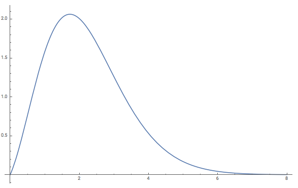
f⁡(x)=x⁡(x+1)Γ⁡(x+2,2​x)−x​Γ​(x+1,2​x)+−4​x3​(x+3)(x+2)​(Γ⁡(x+4,2​x)−3​x​Γ​(x+3,2​x)+2​x2​Γ​(x+2,2​x))\begin{split}f(x)=&\frac{x(x+1)}{\Gamma(x+2,2x)-x\Gamma(x+1,2x)}+\\ &-\frac{4x^{3}(x+3)}{(x+2)(\Gamma(x+4,2x)-3x\Gamma(x+3,2x)+2x^{2}\Gamma(x+2,2x))}\end{split} (15)

for x∈[0,+∞)x\in[0,+\infty). The graph of the function y=f⁡(x)y=f(x) is given in Figure 1 below (the fact that limx→∞f⁡(x)=0\lim_{x\to\infty}f(x)=0 follows by the asymptotic series representation for the incomplete Gamma function given in [2]). So, the value of the costant CC in (13) is equal to the value in (14) if and only if m0=0m_{0}=0 in contrast with the positivity of m0m_{0}, yielding the desired contradiction. The proof of the theorem is complete.
Refer to caption
Figure 1. y=f⁡(x)y=f(x)

∎

References

  • [1] Abramowitz, M., Stegun, I. A. Handbook of Mathematical Functions with Formulas, Graphs, and Mathematical Tables. Dover Publications (1972)
  • [2] Amore, P. Asymptotic and exact series representations for the incomplete Gamma function. Europhysics Letters 71, 1-7 (2005)
  • [3] Arezzo, C., Loi, A. Quantization of Kähler manifolds and the asymptotic expansion of Tian-Yau-Zelditch. Journal of Geo. and Phy. 47, 87-99 (2003)
  • [4] Arezzo, C., Loi, A. Moment maps, scalar curvature and quantization of Kähler manifolds. Comm. Math. Phys. 243, 543-559 (2004)
  • [5] Cahen, M., Gutt, S., Rawnsley, J.H. Quantization of Kähler manifolds I: geometric interpretation of Berezin’s quantization. J. Geophys. 7, 45-62 (1990)
  • [6] Cuccu, F., Loi, A. Global symplectic coordinates on complex domains. J. Geom. Phys. 56, 247-259 (2006)
  • [7] Donaldson, S. Scalar curvature and projective embeddings. I. J. Diff. Geom. 59, 479-522 (2001)
  • [8] Eguchi, T., Hanson A. J. Self-dual solutions to Euclidean gravity. Ann. Physics 120 no. 1, 82-106 (1979)
  • [9] Engliš, M. Weighted Bergman kernels and balancedmetrics. RIMS Kokyuroku 1487, 40-54 (2006)
  • [10] Greco, A., Loi, A. Radial balanced metrics on the unit disk. J. Geom. Phys. 60, 53-59 (2010)
  • [11] Griffiths, P., Harris, J. Principles of Algebraic Geometry. John Wiley & Sons, Inc. (1978)
  • [12] Loi, A., Mossa, R. Berezin quantization of homogeneous bounded domains. Geom. Dedicata 161, 119-128 (2012)
  • [13] Loi, A., Salis, F., Zuddas, F. Two conjectures on Ricci-flat Kähler metrics. Math. Zeit. 1, 1-15 (2018)
  • [14] Loi, A., Zedda, M. Balanced metrics on Cartan and Cartan-Hartogs domains. Math. Z. 270, no. 3-4, 1077-1087 (2012).
  • [15] Loi, A., Zedda, M. Kähler immersions of Kähler manifolds into complex space forms. Lectures Notes of the Unione Matematica Italiana, Springer (2018).
  • [16] McDuff, D. Salamon, D. Introduction to Symplectic Topology. Oxford (2017)
  • [17] Rawnsley, J. Coherent states and Kähler manifolds. Q. J. Math. Oxford (2) 28, 403-415 (1977)