Haze Density Estimation via Modeling of
Scattering Coefficients of iso-depth regions
Abstract
Vision based haze density estimation is of practical implications for the purpose of precaution alarm and emergency reactions toward disastrous hazy weathers. In this paper, we introduce a haze density estimation framework based on modeling of scattering coefficients of iso-depth regions. A haze density metric of Normalized Scattering Coefficient (NSC) is proposed to measure current haze density level with reference to two reference scales. Iso-depth regions are determined via superpixel segmentation. Efficient searching and matching of iso-depth units could be carried out for measurements via unstationary cameras. A robust dark SP selection method is used to produce reliable predictions for most out-door scenarios.
Index Terms:
scattering coefficient, dark channel, iso-depth regionsI Background Introduction
Extreme weather hazards happens more often these days due to climate changes and increased human industrial activities, and one of most notorious of them is haze. When haze happens, dust, smoke and other dry particles obscure the clarity of the sky, impeding human vision, causing respiratory diseases, and most dangerously, it could cause traffic and industrial accidents.
For the purpose of precaution alarm and emergency reactions for the disastrous hazy weather, haze density measurement is of practical importance. The standard solution is to use a haze meter, which measures the amount of light that is diffused or scattered when passing through a transparent material. Haze density (or usually referred to as see through quality) is measured with a narrow angle scattering test in which light is diffused in a small range with high concentration. This test measures the clarity with which finer details can be seen through the object being tested [1]. The haze meter also measures total transmittance. Total transmittance is the measure of the total incident light compared to the light that is actually transmitted.
Since the haze conditions usually change fast, and the distribution of haze in a wider area is commonly uneven, a vision based haze density estimation solution is of practical implications. In this paper, we introduce a haze density estimation framework based on modeling of scattering coefficients of iso-depth regions. A density metric of Normalized Scattering Coefficient (NSC) is proposed to measure current haze density level with reference to two reference scales. Iso-depth regions are determined via superpixel segmentation. Efficient searching and matching of iso-depth units could be carried out for measurements via unstationary cameras. A robust dark SP selection method is used to produce reliable predictions for most out-door scenarios.
I-A The Atmospheric Model for Vision through Haze
The foggy day image appearance is the combined result of attenuated scene radiation and transmitted airlight, whose extents both depend on the scene depth [2]. The classic physical model for atmospheric vision is shown in Eqn. (1) :
| (1) |
where is the camera captured hazy image, is the atmospheric light (referred to as airlight onwards). is the normalized radiance of a scene point, which is a function of the scene point reflectance. The scene albedo is also related to the sky illumination spectrum and intensities. is independent from the weather condition, and it is the haze-free image that we aim to recover.
The physical model in Eqn. (1) describes the two physical phenomena involved when the light propagates to the camera: propagation attenuation , and airlight scattering . denotes the scene point’s transmission rate:
| (2) |
which is a exponential function related to the scene depth , and the scattering coefficient . The scattering coefficient represents the ability of a unit volume of atmosphere to scatter light in all directions [2], and it directly determines the level of visual degradation the haze could cause to a given scene. Larger causes scene radiance to attenuate fast, and scatters the airlight more visibly towards the camera, which results in a contrast compromised and slightly over-exposed capture.
II Proposed Algorithm
In this work, we propose a haze density estimation framework based on the scattering coefficient related to two given references. Given two captures of a target scene captured at two different whether conditions (different scattering coefficients , ). Suppose the camera is stationary and the scene content is static at the moment. The captured hazy images conform to the model in Eq. (1):
| (3) | |||
Eliminating , we get:
| (4) |
Based on the two captures and , we can calculate the airlight intensities and based on the algorithms described in [3, 4]. The normalized depth can now be directly calculated.
II-A Metric for Haze Density Measurement
If given the value of and as reference haze density level, when given another arbitrary scene of a different weather condition (still assume that the camera is stationary and the scene content is static), we aim to estimate the relative ratio of the current with respect to the reference scattering coefficients [, ]. We define the normalized scattering coefficient (NRC) as:
| (5) |
gives a direct indication how heavy the current haze is in a scale of given the two input as reference. The reference input with lighter haze makes scale ”0”, while the heavier one marks the scale ”1”.
To estimate the NRC of an arbitrary input hazy image , according to Eq. (4) and (5), we need to find regions between the two reference images and the target input are iso-depth. For these iso-depth regions, depth values in Eq. (4) could be eliminated, and the NRC can be directly calculated as:
| (6) |
where is the estimated airlight for .
It is worth noting that NRC is only a proposed indicator of this work. Any other indicator that is linearly proportionate to the scattering coefficient can be conveniently fitted into our estimation framework.

II-B Segmentation of Iso-depth Regions
According to Eq. (4), we need to find iso-depth pixels to robustly calculate the scattering coefficients. We proposed to use SuperPixel (SP) segmentation for this purpose. The concept of SP is to group pixels into perceptually meaningful atomic regions [6, 7, 8, 9]. Boundaries of SP usually coincide with those of the scene objects. The SPs are very adaptive in shape, and are more likely to segment uniform depth regions compared with rectangular units.
In this work, we can assume that the pixels inside each SP are iso-depth. We can estimate a robust NRC value for the SP based on the NRC of each SP pixel :
| (7) |
Here, is the SP index. Suppose there are SPs in total. The median filter helps to suppress noisy estimations. A NRC can be estimated for each SP.
II-C Robust Selection of Dark SPs
Based on the assumptions of Dark Channel Prior [3, 10], pixels with smaller dark channel values are more likely to be close to the camera in distance. Regions with brighter dark channels (such as the sky region) tend to produce noisy and over-estimated scene depth. Therefore, we only select a set of SPs whose median dark channel value is below a given threshold to form a subset from all the SPs.
| (8) |
The set is used to estimate the NRC for the whole image:
| (9) |
II-D Captures with Unstationary Caemras and Dynamic Scenes
Until now we are holding the assumption that the cameras used to capture the reference images, and the test input image are strictly stationary, and that the scene contents are static. Such conditions can be hardly meet in practical scenarios.
Based on the SP segmentation, we can first carry out content search and match procedure following global frame alignment as introduced in [6] and [11, 12]. A group of content aligned SPs between the reference and test images will be found, and all the procedures introduced above can be easily fit into a local processing framework based on these aligned SPs. As have been explained in [6], the SP matching operation is robust to both camera motion, and scene content dynamic changes.
III Model Evaluation
In this section, we evaluate the efficiency of the proposed haze density estimation framework.
III-A Synthesis of Hazy Images
First, we synthesized hazy images with image from the dataset by Fattal et al. [5]. The thumbnails for the 11 images in the dataset is shown in Fig. 2. The dataset contains both out-door and in-door scenes, and provides ground truth transmission maps for all scenes.
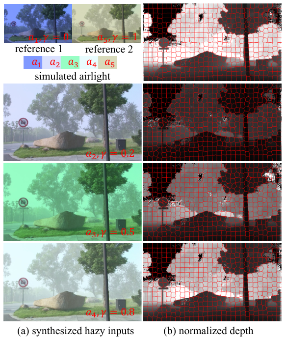
To synthesize haze under different illumination conditions, we used five different airlight values with varying color tones and intensities as specified in Table I. The five airlight colors () are visualized on the top-left figure in Fig. 1.
| Channel | |||||
| R | 128 | 219 | 153 | 234 | 217 |
| G | 154 | 226 | 255 | 253 | 219 |
| B | 255 | 255 | 198 | 255 | 188 |
Based on the haze model defined in Eq. (1) and (2), we set the scattering coefficients at 11 different levels: , which covers the range from light haze to very heavy haze. Consequently, we have synthesized hazy images for each input in the dataset from Fig. 2. Fig. 1(a) shows five different synthesis outcomes with different airlight and NRC configurations for the image road1. Although the airlight is of different color tones, it can be observed that larger values correspond to heavier haze.
We choose the parameter pair as the synthesis parameter for the first reference input, and choose for the second reference input. The experiment results shown hereafter use the same reference settings for all images of the dataset [5].
Fig. 1(b) shows the calculated normalized depth maps for the image road1 that corresponds to the hazy images on the left. As can be seen, different haze levels () result in different normalized depth maps. However, the normalized depth values are similar in each SP (iso-depth regions).
III-B Evaluation of Dark SP Selection
In this sub-section, we evaluate the necessity of the selection of dark SPs as explained in Sec. II-C. We compare the estimated NRC values against the ground truth with or without the dark SP selection step on the data church. The results are shown in Fig. 3.
As can be seen, the results with dark SP selection obviously conforms better to the diagonal line, which represents the ground truth NRC value. The estimation without filtering of dark SPs over-estimates the NRC, especially for light haze conditions.
III-C Evaluation of Density Prediction Precision
In this sub-section, we show the NRC estimation results against ground truth for the data church, lawn1, lawn2, mansion, road1, and road2. As can be observed from Fig. 2, these data are all out-door scenes, therefore the airlight can be better estimated. The results are shown in Fig. 4(a), as can be seen, the NRC plots conform very well to the ground truth NRC values, which validates the efficiency of the proposed haze density estimation framework for out-door scenes.
III-D In-door Failing Cases
For in-door scenes such as couch, flower1, flower2, mobius, and raindeer, the prediction precision is now so good as shown in Fig. 4(b). We noticed that the limitation is mainly caused by incorrectly under-estimated airlight values. Since these scenes are captured in-doors, such error is understandable, since no sky regions exists.
For these in-door cases (which we don’t believe will happen in real world applications), a specialized airlight estimation algorithms can be designed to more accurately calculate the illumination source intensity, however we believe it is out of the scope of the topic discussed in this paper.
IV Conclusions
In this paper, we have introduced a haze density estimation framework based on modeling of scattering coefficients of iso-depth regions. A density metric of Normalized Scattering Coefficient (NSC) is proposed to measure current haze density level with reference to two reference scales. Iso-depth regions are determined via superpixel segmentation. Efficient searching and matching of iso-depth units could be carried out for measurements via unstationary cameras. A robust dark SP selection method is used to produce reliable predictions for most out-door scenarios. Any other haze density metric models that are linearly proportionate to the scattering coefficients can be easily fitted into our estimation framework.
References
- [1] B. Geometries and S. Abrasion, “Standard test method for haze and luminous transmittance of transparent plastics,” ASTM Int, vol. 1, pp. 1–7, 2012.
- [2] S. G. Narasimhan and S. K. Nayar, “Vision and the atmosphere,” International Journal of Computer Vision, vol. 48, no. 3, pp. 233–254, Jul 2002.
- [3] K. He, J. Sun, and X. Tang, “Single image haze removal using dark channel prior,” in IEEE Conference on Computer Vision and Pattern Recognition, June 2009, pp. 1956–1963.
- [4] J. Chen and L.-P. Chau, “Heavy haze removal in a learning framework.”
- [5] R. Fattal, “Dehazing using color-lines,” ACM Transactions on Graphics, vol. 34, no. 1, p. 13, 2014.
- [6] J. Chen, C.-H. Tan, J. Hou, L.-P. Chau, and H. Li, “Robust video content alignment and compensation for rain removal in a cnn framework,” IEEE Conference on Computer Vision and Pattern Recognition, 2018.
- [7] R. Achanta, A. Shaji, K. Smith, A. Lucchi, P. Fua, and S. Susstrunk, “SLIC superpixels compared to state-of-the-art superpixel methods,” IEEE Transactions on Pattern Analysis and Machine Intelligence, vol. 34, no. 11, pp. 2274–2282, 2012.
- [8] M. Van den Bergh, X. Boix, G. Roig, B. de Capitani, and L. Van Gool, SEEDS: Superpixels Extracted via Energy-Driven Sampling. Springer Berlin Heidelberg, 2012, pp. 13–26.
- [9] Z. Li and J. Chen, “Superpixel segmentation using linear spectral clustering,” in IEEE Conference on Computer Vision and Pattern Recognition, Jun. 2015, pp. 1356–1363.
- [10] J. Chen and L. P. Chau, “An enhanced window-variant dark channel prior for depth estimation using single foggy image,” in IEEE International Conference on Image Processing, Sept 2013, pp. 3508–3512.
- [11] C.-H. Tan, J. Chen, and L.-P. Chau, “Dynamic scene rain removal for moving cameras,” in International Conference on Digital Signal Processing. IEEE, 2014, pp. 372–376.
- [12] J. Chen and L.-P. Chau, “Rain removal from dynamic scene based on motion segmentation,” in IEEE International Symposium on Circuits and Systems. IEEE, 2013, pp. 2139–2142.