Temperature-field phase diagram of the two-dimensional dipolar Ising ferromagnet
Abstract
We study field-induced phase transitions in the two-dimensional dipolar Ising ferromagnet with a specific ratio between the exchange and dipolar constants, , which exhibits a stripe-ordered phase with the width of one lattice unit at low temperatures without magnetic field. By using a mean-field (MF) approximation and a Monte Caro (MC) method with the stochastic-cutoff algorithm, which is an simulation method, we show the temperature-field phase diagrams. In the MC study the orientational order and the structure factor are evaluated. Second-order transition points are determined by a finite-size-scaling analysis and first-order transition points are identified by the analysis of the energy histogram. Although both the MF and MC phase diagrams consist of wide regions of several stripe-ordered phases and narrow regions between them characterized by complicated stripe patterns, they show qualitative and quantitative differences in possible phases and phase boundaries. In the MF phase diagram, three main stripe-ordered phases exhibit a nesting structure, while in the MC phase diagram, two main stripe-ordered phases are located separately, which causes a characteristic field-induced reentrant transition of the orientational order.
I Introduction
Thin magnetic films have attracted much attention in their possible applications such as magnetic recording [1]. They show a variety of ordering processes with stripe states, reorientation transitions, etc [2, 3, 4, 5]. The origin of the complexity of the phenomena is the competition between short-range exchange and long-range dipolar interactions.
The two-dimensional (2D) dipolar Ising ferromagnet has been intensively studied to catch the essence of the phenomena in the strong anisotropy limit. The zero-field phase diagram as a function of temperature and the ratio between the exchange and dipolar constants (see eq. (1)) has been focused on [6, 7, 8, 9, 10, 11, 12, 14, 13, 15, 16, 17, 18]. The dipolar interaction leads to the antiferromagnetic (AF) ground state [7], while the Ising ferromagnetic exchange interaction causes the ferromagnetic ground state. Hence frustration affects the ordering process when the two interactions coexist.
MacIsaac et al. reported [7] that the ground state changes at from the AF state to a stripe-ordered state, in which neighboring stripes have opposite magnetizations along the axis. On the other hand, Rastelli et al. pointed out [12] that the model exhibits irregular checkerboard configurations for between the AF and stripe-ordered ones. They also presented the region of for the stability of stripe-ordered phases, e.g., the stripe-ordered phase with the stripe width of one lattice unit, , is stable for . The width of the stripe becomes larger with increasing [7, 12].
At finite temperatures phase transitions between the stripe phases and the disordered (D) phase (or tetragonal liquid (TL) phase) occur, in which -rotational symmetry is broken. It has been clarified that the phase transitions between the stripe-ordered phase with the width and the D (TL) phase are mainly of first order [9, 11, 12], and the nematic phase [19] partially exists between the two phases. The phase transition between the stripe-ordered phase with and the D (TL) phase is still open to debate, namely the phase boundary is a second-order line or the second-order and first-order lines merge at some on the phase boundary [11, 12, 10, 15, 17, 18].
The 2D dipolar Ising ferromagnet also shows field-induced phase transitions [20, 21]. Díaz-Mendez and Mulet investigated the field-temperature phase diagram for [22], which gives the alternating stripes of the width of two lattice units at low temperatures without magnetic field. They presented perfect stripes, anharmonic stripes, bubbles, and ferromagnetic phases with increasing the field at low temperatures. They also pointed out that the phase transition between the bubble and ferromagnetic phases looks like the Berezinskii-Kosterliz-Thouless (BKT) one [23, 24].
In the present study we focus on the model (1) with , in which the ground state configuration without magnetic field is the perfect alternating stripes with the width of . We investigate field-induced phase transitions but do not concentrate on the identification of the bubble phase at present because the correlation length shows an exponential divergence and furthermore logarithmic corrections are accompanied in the BKT phase transition, and precise detection of the BKT transition generally requires very large-scale simulations.
Naive MC algorithms require computational time for simulation of long-range interaction systems such as dipolar systems, since the number of the interactions is . This causes difficulty in the simulation of large system sizes. To overcome this difficulty, several MC algorithms have been proposed [25, 26, 27]. In the present study we adopt the stochastic cutoff (SCO) method proposed by Sasaki and Matsubara [25]. This algorithm was first introduced to a Heisenberg dipolar system, in which the SCO procedure was applied to all dipolar interactions. To realize an efficient MC sampling in the dipolar Ising system with the SCO algorithm, we tune the range (number) of the interactions to which this algorithm is applied.
The rest of the paper is organized as follows. The model is presented in Sec. II. A mean-field (MF) approximation is performed and the MF phase diagram is given in Sec. III. In Sec. IV the phase diagram is studied by the MC simulation. Sec. V is devoted to the summary of the paper including the comparison between the MF and MC phase diagrams. In Appendix A, a tricritical point in the MF phase diagram is derived. In Appendix B, the SCO method and the realization of efficient sampling for the dipolar Ising system with the use of the SCO method are briefly explained.
II Model
The Hamiltonian of the 2D dipolar Ising ferromagnet is
| (1) |
The spin variable takes (up) or (down), perpendicular to the 2D plane. Here is the ratio between the exchange and dipolar constants, and is the magnetic field. The distance between sites and , , is measured in units of the lattice constant. The first sum runs over all pairs of nearest-neighbor spins and the second one over all pairs of spins. We focus on square-lattice systems with sites.
III Mean-field analysis
First we investigate the phase diagram of the system (1) using a MF approximation. Here we assume that the magnetization is uniform in each column in the system of columns and stripes have a period of columns [13, 11]. The self-consistent equations for the system (1) are given by
| (2) |
where is the inverse temperature, i.e., . We set from now on. Here is the average per-site magnetization at the -th row () and
| (3) |
where is defined as
| (4) |
with integers and .


We classify stripe phases by using the notation introduced in Ref. [11]: , in which is the width of a stripe and is the number of consecutive stripes with the same width . We consider a stripe as a region which has a uniform magnetization. Examples of the ground-state configurations of stripe phases are given in Fig. 1. It should be noted that a phase with 1-row stripe is written as (Fig. 1 (a)). In the present study we investigate stripe phases by evaluating the free energies for the solutions of the self-consistent field (SCF) equations (2).
We solve the SCF equations (2) numerically. We calculate up to in most cases and to for a part of complicated phases (see below). In the summations about and in eqs. (3) and (4), we calculate up to and . We determine stripe phases by comparing the stabilities of the free energies for the stable solutions:
| (5) | |||||
Details of the MF phase diagram are given in Figs. 2 (a)-(c). The system is ferromagnetic at high fields and low temperatures, while it is disordered at low fields and high temperatures. In the both states the orientational order is broken and they are not distinguishable. Here we call them “uniform phase”.


In Fig. 2 (a), , , and phases are stable in wide regions. We find that the transition between the and uniform phases is of second order at low fields (), while it is of first order at high fields (), and there exists a tricritical point at (see Appendix A). The other phase transitions are of first order.
IV Monte Carlo study
The MF approach neglects thermal fluctuation effects, and it generally leads to the overestimation of transition temperatures and fields and often fails to estimate the type of phase transitions, e.g., first order or second order. In this section we study the phase diagram of the system (1) by MC simulations based on the SCO algorithm [25]. For efficient MC sampling for the dipolar Ising system, we tune the range of the dipole interactions to which the SCO is applied (see Appendix B).
We take Monte Caro steps (MCS) for equilibration and MCS for measurement at each temperature (or magnetic field) in gradual change of temperature (or magnetic field) staring from random initial configurations. For Figs. 5 and 7, we take MCS for equilibration and MCS for measurement. We obtain physical quantities by averaging over independent 48 measurements with different random number sequences. For Fig. 7 the average physical quantity is estimated by independent 4 measurements.
In order to exclude the effect of edges in the model with long-range interactions (1), we adopt a replica method tiling replicas of the original system [16, 17] with periodic boundary conditions. Here we tile 20012001 replicas.
To detect stripe phases, we define the following order parameter [6, 10],
| (6) |
where and are the numbers of vertical and horizontal bonds between nearest neighbor anti-aligned spins, respectively. This order parameter detects -rotational symmetry breaking, and if each row or column is fully ordered alternately, i.e., alternation of and , we have . Here stands for the statistical average of the quantity . For ferromagnetically-ordered or disordered states, we have .


We investigate second-order phase transitions by using the fourth-order Binder cumulant [28] of :
| (7) |
The transition temperature is obtained by the intersection of the curves for different system sizes. Figs. 3 (a) and (b) depict at (a) and (b) for several system sizes, and the curves cross at and for and , respectively to exhibit second-order phase transitions. Similar crossings are also observed at all the points denoted by circles in Fig. 6 for .


For first-order transitions, we investigate the histogram of the total energy as a function of and . If the phase transition is of first order, the histogram should have two peaks around the transition temperature, while it should have one peak for second-order transitions. Indeed no double peaks are observed around at and . We plot energy histograms around the transition temperature at for in Fig. 4 (a). Double peaks around and are found in the region between and 0.3092. The lower-energy peak is dominant at , and the higher-energy peak grows and becomes dominant with increasing temperature up to . In Fig. 4 (b) we compare the double-peak structure for and . The peaks become sharper as the system size increases. These observations are clear evidence for the first-order transition.
To specify the stripe patterns, the structure factor is investigated:
| (8) |
| (9) |
Here is the position of site . In the present study, the system has -rotational symmetry and we measure . In Fig. 5 the field dependence of is plotted at . At , has a peak at , which indicates the phase. s at and show peaks at and , which suggests the phase with the -lattice-unit period. We perform the same analyses at different temperatures and fields, and obtain the MC phase diagram displayed in Fig. 6.


The phase at low fields and the phase at high fields are main contribution to the phase diagram, and there exists a region characterized by complicated phases between these two phases, as we see below.
The MF approximation is rigorous at under the assumption of stripe-ordered phases with the restriction, and we substitute the MF phase boundaries of the and phases at , denoted by stars in Fig. 6, for the MC ones. We sketch rough phase boundaries between the , complicated, and phases there.
We find that the phase transition between the and uniform phases is of second order. Concerning this phase transition at , there have been controversial results about the region of for the second-order transition line in the vicinity of in the zero-field MC phase diagram [11, 18, 17, 15]. First-order transition was pointed out at in several studies [11, 12, 10]. On the other hand, it has been recently shown that the second-order transition line exists up to [15, 17, 18]. Our result at is consistent with the latter, and our estimate is comparable to in Ref. [17].
For the phase at higher fields, we obtain clear evidence for the first-order transition in the energy-histogram analysis for the filled squares in Fig. 6, while we do not observe sharp double peaks for the open squares within the present system sizes. We expect the full first-order phase transition between the and uniform phases, but tricritical point(s) might exist between the filled and open squares in Fig. 6.
We see some complicated phases between the and phases at the intermediate fields. The Binder plots for the phase boundaries between these phases and the disordered phase indicate second-order transition as depicted in Fig. 3 (b). At has peaks around and (and weakly around and ), which is consistent with the phase with the -lattice-unit period. It is difficult to identify the patterns of the phases between the and phases and between the and phases because peaks of are too weak and broad (e.g. at ) and positions of them shift continuously as the field changes.
The MC phase diagram is characterized by the dominant and phases and the narrow region of complicated phases. This structure brings a field-induced reentrant transition of the phase, i.e., uniform to to uniform phase. As an example, the field dependence of the order parameter at for is shown in Fig. 7.

V Summary
We investigated the temperature-field phase diagrams for in the two-dimensional dipolar Ising ferromagnet by using the MF and MC methods. In the MC method we adopted the SCO algorithm, efficient to simulations of long-range interaction systems. In the MC study the finite-size-scaling method was applied for the second-order phase transition and the energy histogram analysis was performed for the first-order phase transitions. We found both qualitative and quantitative differences between the MF and MC phase diagrams, which is due to the thermal fluctuation and frustration effects.
The critical temperature at zero field is in the MF analysis, while that in the MC method is . The phase in the MF phase diagram does not exist in the MC phase diagram, and the upper transition filed of the phase is much reduced in the MC phase diagram. There is a tricritical point in the phase transition between the and uniform phases in the MF analysis. On the other hand, this transition is of second order in the MC analysis. In the MF phase diagram the phase neighbors the phase, and the phase neighbors the . The , , and phase boundaries show a nesting structure.
On the other hand, in the MC phase diagram and phases do not neighbor and a nesting structure does not exist. Such qualitative differences between the MF and MC phase diagrams have been found in various frustrated systems such as the triangular Ising model and its extension [29, 30]. The reduction of or in the MC method is partially attributed to the thermal fluctuation effects.
In the MC phase diagram there exist a small region of complicated stripe phases between the regions of and phases. This feature causes the field-induced reentrant transition of the phase: uniform to to uniform phase. So far field-induced reentrant transitions have not been observed in the dipolar Ising system such as the case of [22]. We first found a field-induced reentrant transition of a stripe phase, i.e., uniform to to uniform phase. This is a nontrvial characteristic in the model with .
Acknowledgments
The present work was supported by Grants-in-Aid for Scientific Research C (No. 17K05508) from MEXT of Japan, and the Elements Strategy Initiative Center for Magnetic Materials (ESICMM) under the outsourcing project of MEXT. Part of numerical calculations were performed on the Numerical Materials Simulator at National Institute for Materials Science.
Appendix A Tricritical point in the MF phase diagram
We find a tricritical point in the phase transition between the and uniform phases. Using the translational symmetry , the free energy (5) for is rewritten as a function of as follows.
| (10) | |||||
In the phase transition from to uniform phase, changes from to . Hence, the tricritical point is obtained from the following conditions:
| (11) |
and we have the relations,
| (12) |
and
| (13) |
| (14) |
Solving the SCF equations with the relations, the tricritical point is given as and , at which .
Appendix B SCO method for the Ising dipolar model
In this appendix we briefly explain the implementation of the SCO algorithm suitable for the Ising dipolar system. The SCO method [25] is based on the stochastic potential switching (SPS) algorithm [31, 32] with switching time, which realizes computational time for simulation of dipolar systems.
In the SPS algorithm long-range interaction is stochastically switched to with a probability or to with . The potential can be chosen arbitrarily. Here is written as
| (15) |
where
| (16) |
and is a constant equal to or greater than the maximum value of . The potential is given by
| (17) |
In the SCO method for the dipolar Heisenberg model, this SPS procedure is applied to all dipolar interactions with and is not applied to the nearest-neighbor Heisenberg couplings. Namely, all nearest-neighbor Heisenberg interactions and some dipolar interactions selected by the SPS procedure are considered for the update of the state in one MC step.
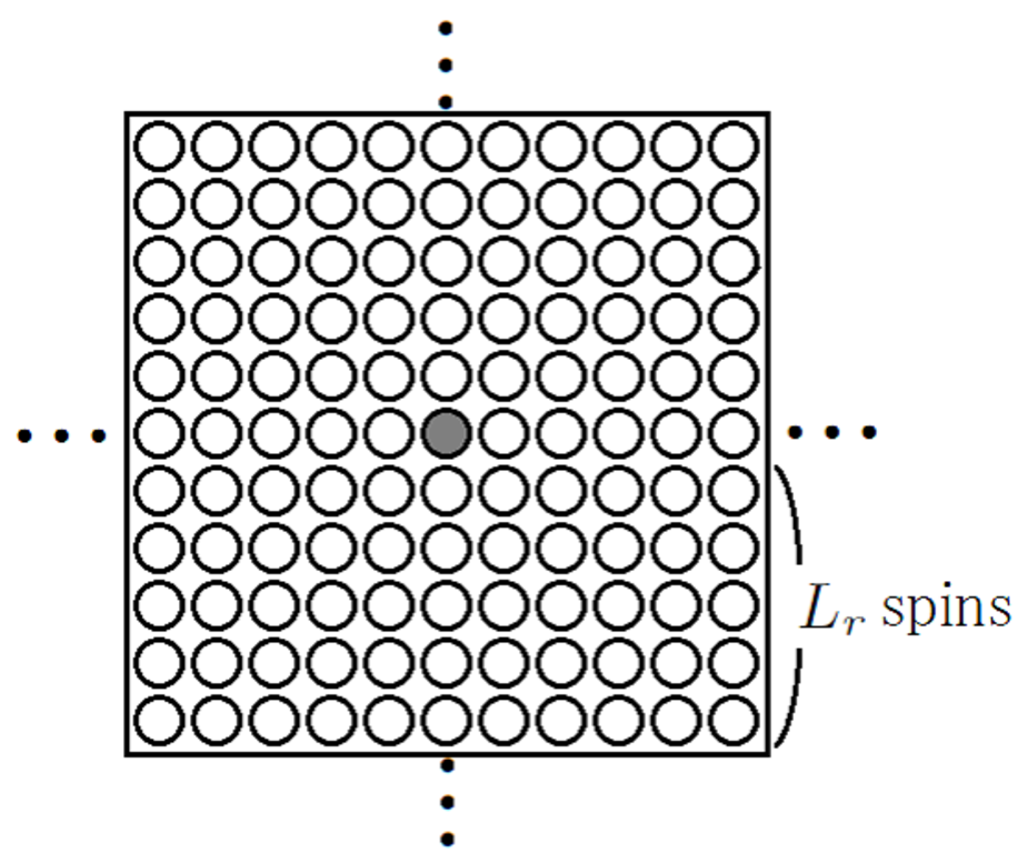
Here we tune the number of the dipolar interactions to which the SPS procedure is applied. We show that this tuning is useful for the acceleration of the relaxation in the Ising dipolar model. For a single spin flip for the spin denoted by the filled circle in Fig. 8, the SPS procedure is not applied to the dipolar interactions around the spin within the range of sites (open circles in Fig. 8) , i.e., these interactions are always counted for the single spin flip in the same way as the nearest-neighbor Ising interactions.
We give dependence of the relaxation curves of in Fig. 9. The case corresponds to the original SCO method and we find drastic reduction of the relaxation time for . We adopted , which provides enough efficiency in the MC sampling for the present work.
This improvement is attributed to the discretized spin state (up or down) of the Ising spin. The dipolar interaction in eq. (1),
| (18) |
takes two values, i.e., and for ferromagnetic () and antiferromagnetic () spins, respectively. Defining , in which , and for ferromagnetic and antiferromagnetic spins, respectively. In the present study we take .
Because
| (19) |
for ferromagnetic spins is much larger than that for antiferromagnetic spins for smaller and lower . Namely the probability for selecting for ferromagnetic spins is much smaller than that for antiferromagnetic spins. This large difference of causes a deviation of the potential switching pattern and inefficiency of the MC sampling.

References
- [1] S. D. Bader, Rev. Mod. Phys 78, 1 (2006).
- [2] R. Allenspach, M. Stampanoni, and A. Bischof, Phys. Rev. Lett. 65, 3344 (1990).
- [3] A. B. Kashuba and V. L. Pokrovsky, Phys. Rev. B 48, 10335 (1993).
- [4] K. De’Bell, A. B. MacIsaac, and J. P. Whitehead, Rev. Mod. Phys. 72, 225 (2000).
- [5] O. Portmann, A. Vaterlaus, and D. Pescia, Nature 422, 701 (2003).
- [6] I. Booth, A. B. MacIsaac, J. P. Whitehead, and K. De’Bell, Phys. Rev. Lett. 75, 950 (1995).
- [7] A. B. MacIsaac, J. P. Whitehead, M. C. Robinson, and K. De’Bell, Phys. Rev. B 51, 16033 (1995).
- [8] J. H. Toloza, F. A. Tamarit, and S. A. Cannas, Phys. Rev. B 58, R8885 (1998).
- [9] E. Rastelli, S. Regina, and A. Tassi, Phys. Rev. B 73, 144418 (2006).
- [10] S. A. Cannas, M. F. Michelon, D. A. Stariolo, and F. A. Tamarit, Phys. Rev. B 73, 184425 (2006).
- [11] S. A. Pighin and S. A. Cannas Phys. Rev. B 75, 224433 (2007).
- [12] E. Rastelli, S. Regina, and A. Tassi, Phys. Rev. B 76, 054438 (2007).
- [13] A. Vindigni, N. Saratz, O. Portmann, D. Pescia, and P. Politi, Phys. Rev. B 77, 092414 (2008).
- [14] L. G. Rizzi and N. A. Alves, Physica B 405, 1571 (2010).
- [15] J. S. M. Fonseca, L. G. Rizzi, and N. A. Alves, Phys. Rev. E 86, 011103 (2012).
- [16] R. Rüger and R. Valentí, Phys. Rev. B 86, 024431 (2012).
- [17] C. M. Horowitz, M. A. Bab, M. Mazzini, M. L. Rubio Puzzo, and G. P. Saracco, Phys. Rev. E 92, 042127 (2015).
- [18] M. A. Bab, C. M. Horowitz, M. L. Rubio Puzzo, and G. P. Saracco, Phys. Rev. E 94, 042104 (2016).
- [19] Ar. Abanov, V. Kalatsky, V. L. Pokrovsky, and W. M. Saslow, Phys. Rev. B 51, 1023 (1995).
- [20] T. Garel and S. Doniach, Phys. Rev. B 26, 325 (1982).
- [21] J. Arlett J. P. Whitehead, A. B. MacIsaac, and K. De’Bell, Phys. Rev. B 54, 3394 (1995).
- [22] R. Díaz-Mendez and R. Mulet, Phys. Rev. B 81, 184420 (2010).
- [23] V. L. Berezinskii, Sov. Phys. JETP 32, 493 (1971); 34, 610 (1972).
- [24] J. M. Kosterlitz and D. J. Thouless, J. Phys. C 6, 1181 (1973).
- [25] M. Sasaki and F. Matsubara, J. Phys. Soc. Jpn. 77, 024004 (2008).
- [26] K. Fukui and S. Todo, J. Comput. Phys. 228, 2629 (2009).
- [27] T. Hinokihara, M. Nishino, Y. Toga, and S. Miyashita, Phys. Rev. B 97, 104427 (2018).
- [28] K. Binder, Phys. Rev. Lett. 47, 693 (1981).
- [29] M. Mekata, J. Phys. Soc. Jpn. 42, 76 (1977).
- [30] D. P. Landau, Phys. Rev. B 27, 5604 (1983).
- [31] C. H. Mak, J. Chem. Phys. 122, 214110 (2005).
- [32] C. H. Mak and A. K. Sharma, Phys. Rev. Lett. 98, 180602 (2007).