跳到论文正文
W Papers独立论文阅读器 arXiv:1808.05895 论文正文 计算阅读时间 · 0%
引用这篇论文根据当前论文元数据生成,正式投稿前建议核对。


License: arXiv.org perpetual non-exclusive license
arXiv:1808.05895v1 [stat.ME] 17 Aug 2018

Estimating and accounting for unobserved covariates in high dimensional correlated data

Chris McKennan Address: Department of Statistics, University of Chicago, Chicago, IL, USA. Email: cgm29@uchicago.edu    Dan Nicolae Address: Department of Statistics, University of Chicago, Chicago, IL, USA.
Abstract

Many high dimensional and high-throughput biological datasets have complex sample correlation structures, which include longitudinal and multiple tissue data, as well as data with multiple treatment conditions or related individuals. These data, as well as nearly all high-throughput ‘omic’ data, are influenced by technical and biological factors unknown to the researcher, which, if unaccounted for, can severely obfuscate estimation and inference on effects due to the known covariate of interest. We therefore developed CBCV and CorrConf: provably accurate and computationally efficient methods to choose the number of and estimate latent confounding factors present in high dimensional data with correlated or nonexchangeable residuals. We demonstrate each method’s superior performance compared to other state of the art methods by analyzing simulated multi-tissue gene expression data and identifying sex-associated DNA methylation sites in a real, longitudinal twin study. As far as we are aware, these are the first methods to estimate the number of and correct for latent confounding factors in data with correlated or nonexchangeable residuals. An R-package is available for download at https://github.com/chrismckennan/CorrConf.

keywords
Latent factors, batch effects, unwanted variation, correlation, multi-tissue, cell-type heterogeneity

1 Introduction

The development of high-throughput biotechnologies has provided biologists with a cornucopia of genetic, proteomic and metabolomic data that can been used to elucidate the genetic components of many phenotypes and the mediation of environmental exposures. Many of these ‘omic’ data have complex sample-correlation structure, which includes longitudinal data (Baumgart et al., 2016; Agha et al., 2016; McKennan et al., 2018), multi-tissue data (GTEx Consortium, 2017; Yu et al., 2017), data with multiple treatment conditions (Knowles et al., 2018) and data with related individuals (Martino et al., 2013; Tung et al., 2015). Longitudinal studies have even been cited as a critical area of future DNA methylation research to assess the stability of methylation marks over time (Breton et al., 2017; Martin and Fry, 2018a), so it is crucial that suitable methods exist to analyze these data. An important feature of these high-throughput experimental data is the presence of unmeasured factors, which include technical factors like batch variables and biological factors like cell composition, that influence the measured response (Leek et al., 2010; Jaffe and Irizarry, 2014). When unaccounted for, these factors can bias test statistics, reduce power and lead to irreproducible results (Yao et al., 2012; Peixoto et al., 2015). There have been a number of methods developed by the statistical community to estimate and correct for latent factors (Buja and Eyuboglu, 1992; Leek and Storey, 2008; Gagnon-Bartsch and Speed, 2012; Sun et al., 2012; Gagnon-Bartsch et al., 2013; Houseman et al., 2014; Owen and Wang, 2016; Fan and Han, 2017; Lee et al., 2017; Wang et al., 2017; McKennan and Nicolae, 2018). However, all of these methods make the critical assumption that conditional on both the observed and unobserved covariates, samples are independent with homogeneous residual variances, and tend to perform poorly when these assumptions are violated. The goal of this paper is therefore to provide a provably accurate method to both choose the number of latent factors and estimate them from the measured correlated data precisely enough so that downstream inference on the covariate of interest is as accurate as when the latent variables are observed. To the best of our knowledge, this is the first method to estimate and correct for latent covariates in correlated data.

We use DNA methylation quantified in p≈8×10⁵p\approx 8\times 10^{5} methylation sites (i.e. CpGs) in 183 unrelated individuals at birth and age 7 (n=2×183n=2\times 183) from McKennan et al. (2018) as a motivating data example, although we analyze other methylation data with a more complex covariance structure in Section 5. The aim is to jointly model methylation at birth and age 7 to determine if the effects due to ancestry on methylation levels changed or remained constant over time. If we ignore observed nuisance variables like the intercept, a reasonable model for the methylation at birth and age 7 at CpG gg (𝒚g(0)∈ℝn/2\bm{y}_{g}^{(0)}\in\mathbb{R}^{n/2} and 𝒚g(7)∈ℝn/2\bm{y}_{g}^{(7)}\in\mathbb{R}^{n/2}) in the presence of unobserved covariates 𝑪∈ℝn×K\bm{C}\in\mathbb{R}^{n\times K} (K<<nK<<n, an unknown constant) is

𝒚g\displaystyle\bm{y}_{g} =(𝒚g(0)𝒚g(7))T=𝑿(βg(0)βg(7))T+𝑪ℓg+𝒆g,𝒆g∼N(0,𝑽g)(g=1,…,p)\displaystyle=\left(\bm{y}_{g}^{(0)}\,\bm{y}_{g}^{(7)}\right)^{T}=\bm{X}\left(\beta_{g}^{(0)}\,\beta_{g}^{(7)}\right)^{T}+\bm{C}\bm{\ell}_{g}+\bm{e}_{g},\quad\bm{e}_{g}\sim N\left(0,\bm{V}_{g}\right)\quad(g=1,\ldots,p) (1a)
𝑽g\displaystyle\bm{V}_{g} =ϕg2𝑩1+σg,02𝑩2+σg,72𝑩3(g=1,…,p)\displaystyle=\phi^{2}_{g}\bm{B}_{1}+\sigma_{g,0}^{2}\bm{B}_{2}+\sigma_{g,7}^{2}\bm{B}_{3}\quad(g=1,\ldots,p) (1b)

where 𝑿=𝑨⊕𝑨∈ℝn×2\bm{X}=\bm{A}\oplus\bm{A}\in\mathbb{R}^{n\times 2} and 𝑨∈ℝn/2\bm{A}\in\mathbb{R}^{n/2} gives each individual’s ancestry, 𝑩1∈ℝn×n\bm{B}_{1}\in\mathbb{R}^{n\times n} is a partition matrix that groups samples by individuals and 𝑩2∈ℝn×n\bm{B}_{2}\in\mathbb{R}^{n\times n} and 𝑩3∈ℝn×n\bm{B}_{3}\in\mathbb{R}^{n\times n} are diagonal matrices with ones in the first n/2n/2 and second n/2n/2 diagonal entries, respectively, and zeros everywhere else that capture the potential difference in residual variance at birth and age 7. In order to avoid overestimating the residual variance and biasing our estimates for the effects of interest βg(0)\beta_{g}^{(0)} and βg(7)\beta_{g}^{(7)}, we must first estimate 𝑪\bm{C}. Instead of effectively reducing the sample size by 50% and estimating 𝑪\bm{C} separately at birth and age 7, which risks underestimating KK and subsequently biasing estimates for βg(0)\beta_{g}^{(0)} and βg(7)\beta_{g}^{(7)}, we would ideally estimate KK and subsequently 𝑪\bm{C} using all nn samples, since we expect technical and many biological factors (including cell composition) to affect methylation at both ages. However, naively applying standard methods to choose KK designed for data with independent and identically distributed residuals, like parallel analysis (Buja and Eyuboglu, 1992) and bi-cross validation (Owen and Wang, 2016), will typically overestimate the latent factor dimension to be on the order of the sample size, as they will be unable to distinguish the low dimensional factors 𝑪\bm{C} from the high dimensional random effect. Even if KK were known, the correlation among the residuals obfuscates current state of the art method’s estimates for 𝑪\bm{C}.

Our proposed computationally efficient method uses all of the available data to estimate KK and 𝑪\bm{C} for data whose gene-, methylation-, protein- or metabolite-specific covariance can be written as a linear combination of known positive semi-definite matrices. As we will eventually show, this covariance structure is quite general and includes longitudinal, multi-tissue, multi-treatment and twin studies, as well as studies with individuals related through a kinship matrix. While our ultimate goal is to be able to do inference on the effects of interest that is as accurate as when 𝑪\bm{C} is observed, our method also provides a way to efficiently perform factor analysis in data with correlated or nonexchangeable residuals 𝒆g​1,…,𝒆g​n\bm{e}_{g1},\ldots,\bm{e}_{gn} (g=1,…,pg=1,\ldots,p) and has application in quantitative train loci (QTL) studies (Knowles et al., 2018; McKennan et al., 2018).

We demonstrate the efficacy of our method by showing it selects the correct latent factor dimension with high probability, its estimate for the column space of 𝑪\bm{C} is nearly as accurate as when samples are independent (i.e. 𝑽g\bm{V}_{g} in (1) is a multiple of the identity) and that downstream inference on the effect of interest is asymptotically equivalent to inference with the generalized least squares estimator when 𝑪\bm{C} is known. We also simulate multi-tissue gene expression data with a complex, gene-dependent correlation structure to illustrate our method’s superior performance in both choosing KK and estimating 𝑪\bm{C}.

The remainder of the paper is organized as follows. Section 2 provides a description of and generative model for the data and an overview of our estimation procedure. Section 3 gives a detailed description of our estimation procedure, as well as all relevant theory. We then analyze simulated data in Section 4 and apply our method to a longitudinal DNA methylation dataset with measurements made on pairs of twins to identify CpGs with sex-dependent methylation levels in Section 5. An R package called CorrConf that implements our method to estimate KK and 𝑪\bm{C} is freely available with download instructions provided in Section 7. The proofs of all propositions, lemmas and theorems can be found in the Supplement.

2 Notation and problem set-up

2.1 Basic notation

Define 𝟏n∈ℝn\bm{1}_{n}\in\mathbb{R}^{n} be the vector of all ones and In∈ℝn×nI_{n}\in\mathbb{R}^{n\times n} to be the identity matrix. For any matrix 𝑴∈ℝn×m\bm{M}\in\mathbb{R}^{n\times m}, we define PMP_{M}, PM⟂P_{M}^{\perp} to be the orthogonal projections matrices onto the image and orthogonal complement of 𝑴\bm{M}. If d>0d>0 is the dimension of the null space of 𝑴T\bm{M}^{T}, we define 𝑸M∈ℝn×d\bm{Q}_{M}\in\mathbb{R}^{n\times d} to be a matrix whose columns form an orthonormal basis for the null space of 𝑴T\bm{M}^{T}, i.e. 𝑸MT​𝑴=𝟎\bm{Q}_{M}^{T}\bm{M}=\bm{0}, 𝑸MT​𝑸M=Id\bm{Q}_{M}^{T}\bm{Q}_{M}=I_{d} and 𝑸M​𝑸MT=PM⟂\bm{Q}_{M}\bm{Q}_{M}^{T}=P_{M}^{\perp}. Lastly, 𝑿​=d𝐘\bm{X}\edist\bm{Y} if the two random variables, vectors or matrices 𝑿\bm{X} and 𝒀\bm{Y} have the same distribution.

2.2 A description of and generative probability model for the data

Suppose we measure the expression or methylation 𝒚g∈ℝn\bm{y}_{g}\in\mathbb{R}^{n} (g=1,…,pg=1,\ldots,p) of pp units across nn potentially correlated samples and, when applicable, observe the covariates of interest 𝑿∈ℝn×d\bm{X}\in\mathbb{R}^{n\times d}. Throughout this work, we will assume 𝑿\bm{X} is “well-behaved”, i.e. the smallest and largest eigenvalues of n−1​𝑿T​𝑿n^{-1}\bm{X}^{T}\bm{X} remains bounded above 0 and below a fixed constant. When unobserved factors 𝑪∈ℝn×K\bm{C}\in\mathbb{R}^{n\times K} influence the response, we assume the data 𝒚g\bm{y}_{g} are generated as

𝒚g\displaystyle\bm{y}_{g} =𝑿​𝜷g+𝑪​ℓg+𝒆g,𝒆g∼N⁡(𝟎,𝑽g)​(g=1,…,p)\displaystyle=\bm{X}\bm{\beta}_{g}+\bm{C}\bm{\ell}_{g}+\bm{e}_{g},\quad\bm{e}_{g}\sim N\left(\bm{0},\bm{V}_{g}\right)\,\,(g=1,\ldots,p) (2a)
𝒀\displaystyle\bm{Y} =[𝒚1⋯𝒚p]T=𝜷𝑿T+𝑳𝑪T+𝑬\displaystyle=\left[\bm{y}_{1}\,\cdots\,\bm{y}_{p}\right]^{T}=\bm{\beta}\bm{X}^{T}+\bm{L}\bm{C}^{T}+\bm{E} (2b)
𝑽g\displaystyle\bm{V}_{g} =vg,1​𝑩1+⋯+vg,b​𝑩b​(g=1,…,p)\displaystyle=v_{g,1}\bm{B}_{1}+\cdots+v_{g,b}\bm{B}_{b}\,\,(g=1,\ldots,p) (2c)

where the gthg^{\text{th}} row of 𝜷\bm{\beta}, 𝑳\bm{L} and 𝑬\bm{E} is 𝜷g\bm{\beta}_{g}, ℓg\bm{\ell}_{g} and 𝒆g\bm{e}_{g}, respectively, 𝒆g\bm{e}_{g} and 𝒆g′\bm{e}_{g^{\prime}} are independent for g≠g′g\neq g^{\prime}, the variance multipliers vg,jv_{g,j} (g=1,…,pg=1,\ldots,p; j=1,…,bj=1,\ldots,b) are unknown and 𝑩j∈ℝn×n\bm{B}_{j}\in\mathbb{R}^{n\times n} (j=1,…,bj=1,\ldots,b) are known and describe how the nn samples are related. Lastly, we assume that the variance multipliers 𝒗g=(vg,1⋯vg,b)T\bm{v}_{g}=\left(v_{g,1}\,\cdots\,v_{g,b}\right)^{T} lie in the convex polytope Θ\Theta, defined as

Θ={𝒙∈ℝb:𝑨ℰ𝒙=𝟎,𝑨ℐ𝒙≥𝟎}\displaystyle\Theta=\left\{\bm{x}\in\mathbb{R}^{b}:\bm{A}_{\mathcal{E}}\bm{x}=\bm{0},\bm{A}_{\mathcal{I}}\bm{x}\geq\bm{0}\right\} (3)

where 𝑨ℰ∈ℝNℰ×b\bm{A}_{\mathcal{E}}\in\mathbb{R}^{N_{\mathcal{E}}\times b} and 𝑨ℐ∈ℝNℐ×b\bm{A}_{\mathcal{I}}\in\mathbb{R}^{N_{\mathcal{I}}\times b} are the equality and inequality constraints on 𝒗g\bm{v}_{g}. For example, we may know that certain multipliers must be larger than others, or that the sum of two sets of multipliers must be equal to ensure the marginal variances are the same. Depending on how we parametrize the covariance matrices 𝑽g\bm{V}_{g}, the multipliers can take negative values as long as 𝑽g\bm{V}_{g} is interpretable as a covariance matrix. We lastly note that the form for parameter space Θ\Theta is sufficient for most problems because it assumes one only has prior information about the relative sizes of the variance multipliers (as well as their sign). It is unlikely for practitioner to know the absolute sizes of the multipliers.

In many applications there are other observed covariates 𝒁∈ℝn×r\bm{Z}\in\mathbb{R}^{n\times r} that may influence the response 𝒚g\bm{y}_{g} but whose effects are not of interest. In that case, the model for 𝒚g\bm{y}_{g} would be

𝒚g=𝑿​𝜷g+𝒁​𝒘g+𝑪​ℓg+𝒆g,\displaystyle\bm{y}_{g}=\bm{X}\bm{\beta}_{g}+\bm{Z}\bm{w}_{g}+\bm{C}\bm{\ell}_{g}+\bm{e}_{g},

and we can get back to model (2) by multiplying 𝒚g\bm{y}_{g} by 𝑸ZT\bm{Q}_{Z}^{T}, provided rr does not grow with nn:

𝑸ZT​𝒚g\displaystyle\bm{Q}_{Z}^{T}\bm{y}_{g} =(𝑸ZT​𝑿)​𝜷g+(𝑸ZT​𝑪)​ℓg+𝒆¯g,𝒆¯g∼N⁡(𝟎,𝑽¯g)\displaystyle=\left(\bm{Q}_{Z}^{T}\bm{X}\right)\bm{\beta}_{g}+\left(\bm{Q}_{Z}^{T}\bm{C}\right)\bm{\ell}_{g}+\bar{\bm{e}}_{g},\quad\bar{\bm{e}}_{g}\sim N\left(\bm{0},\bar{\bm{V}}_{g}\right)
𝑽¯g\displaystyle\bar{\bm{V}}_{g} =vg,1​(𝑸ZT​𝑩1​𝑸Z)+⋯+vg,b​(𝑸ZT​𝑩b​𝑸Z).\displaystyle=v_{g,1}\left(\bm{Q}_{Z}^{T}\bm{B}_{1}\bm{Q}_{Z}\right)+\cdots+v_{g,b}\left(\bm{Q}_{Z}^{T}\bm{B}_{b}\bm{Q}_{Z}\right).

Therefore, we assume that the only observed covariates are contained in 𝑿\bm{X}.

Our primary goal is to estimate the column space of 𝑪\bm{C} accurately enough so that inference on 𝜷g\bm{\beta}_{g} is just as accurate as the generalized least squares estimate for 𝜷g\bm{\beta}_{g} when 𝑪\bm{C} is known, and secondary goal is to simply estimate the column space of 𝑪\bm{C} when there are no covariates of interest, i.e. d=0d=0. Since accomplishing the former implies we can achieve the latter, we only consider the case when d≥1d\geq 1.

To estimate 𝑪\bm{C}, we partition the variability of 𝒚1,…,𝒚p\bm{y}_{1},\ldots,\bm{y}_{p} into two pieces: one part explainable by 𝑿\bm{X} and another orthogonal to 𝑿\bm{X}. Specifically, for some positive definite matrix 𝑮∈ℝn×n\bm{G}\in\mathbb{R}^{n\times n} we define

𝒚g1=(𝑿T​𝑮−1​𝑿)−1​𝑿T​𝑮−1​𝒚g=𝜷g+𝛀​ℓg+𝒆g1​(g=1,…,p)\displaystyle\bm{y}_{g_{1}}=\left(\bm{X}^{T}\bm{G}^{-1}\bm{X}\right)^{-1}\bm{X}^{T}\bm{G}^{-1}\bm{y}_{g}=\bm{\beta}_{g}+\bm{\Omega}\bm{\ell}_{g}+\bm{e}_{g_{1}}\,\,(g=1,\ldots,p) (4a)
𝛀=(𝑿T​𝑮−1​𝑿)−1​𝑿T​𝑮−1​𝑪\displaystyle\bm{\Omega}=\left(\bm{X}^{T}\bm{G}^{-1}\bm{X}\right)^{-1}\bm{X}^{T}\bm{G}^{-1}\bm{C} (4b)
𝒚g2=𝑸XT​𝒚g=𝑪⟂​ℓg+𝒆g2,𝒆g2∼N⁡(𝟎,𝑾g)​(g=1,…,p)\displaystyle\bm{y}_{g_{2}}=\bm{Q}_{X}^{T}\bm{y}_{g}=\bm{C}_{\perp}\bm{\ell}_{g}+\bm{e}_{g_{2}},\quad\bm{e}_{g_{2}}\sim N\left(\bm{0},\bm{W}_{g}\right)\,\,(g=1,\ldots,p) (4c)
𝑪⟂=𝑸XT​𝑪\displaystyle\bm{C}_{\perp}=\bm{Q}_{X}^{T}\bm{C} (4d)
𝑾g=∑j=1bvg,j​𝑸XT​𝑩j​𝑸X​(g=1,…,p)\displaystyle\bm{W}_{g}=\sum\limits_{j=1}^{b}v_{g,j}\bm{Q}_{X}^{T}\bm{B}_{j}\bm{Q}_{X}\,\,(g=1,\ldots,p) (4e)
𝒀1=[𝒚11⋯𝒚p1]T=𝜷+𝑳𝛀T+𝑬1,𝒀2=[𝒚12⋯𝒚p2]T=𝑳𝑪⟂T+𝑬2\displaystyle\bm{Y}_{1}=\left[\bm{y}_{1_{1}}\,\cdots\,\bm{y}_{p_{1}}\right]^{T}=\bm{\beta}+\bm{L}\bm{\Omega}^{T}+\bm{E}_{1},\quad\bm{Y}_{2}=\left[\bm{y}_{1_{2}}\,\cdots\,\bm{y}_{p_{2}}\right]^{T}=\bm{L}\bm{C}_{\perp}^{T}+\bm{E}_{2} (4f)

where the gthg^{\text{th}} rows of 𝑬1\bm{E}_{1} and 𝑬2\bm{E}_{2} are 𝒆g1\bm{e}_{g_{1}} and 𝒆g2\bm{e}_{g_{2}}, 𝛀\bm{\Omega} is the weighted least squares regression coefficient for the regression 𝑪\bm{C} onto 𝑿\bm{X} and 𝒚g1\bm{y}_{g_{1}} is the naive weighted least squares estimator for 𝜷g\bm{\beta}_{g} (g=1,…,pg=1,\ldots,p) that ignores 𝑪\bm{C}. We show how to choose the appropriate 𝑮\bm{G} when we provide our estimate for 𝜷g\bm{\beta}_{g} in Section 3.4. 𝑪⟂\bm{C}_{\perp} and 𝒚g2\bm{y}_{g_{2}} lie in the space orthogonal to 𝑿\bm{X}, where the latter no longer depends on 𝜷g\bm{\beta}_{g}. Algorithm 1 below provides a cursory description of how we use the objects defined in (4) to estimate 𝑪\bm{C}.

Algorithm 1
  1. (a)

    Use 𝒀2\bm{Y}_{2} and a cross-validation procedure to estimate KK, the dimension of the column space of 𝑪\bm{C}. This procedure is called CBCV (Correlated Bi-Cross Validation) and is enumerated in Section 3.3.

  2. (b)

    For KK known, use 𝒀2\bm{Y}_{2} to estimate 𝑳\bm{L}, 𝑪⟂\bm{C}_{\perp} and the appropriate 𝑮\bm{G} using an iterative factor analysis procedure we call ICaSE (Iterative Correlation and Subspace Estimation), which we discuss in Section 3.2.

  3. (c)

    Estimate 𝛀\bm{\Omega} using 𝒀1\bm{Y}_{1}, 𝑳^\hat{\bm{L}}, 𝑪^⟂\hat{\bm{C}}_{\perp} and 𝑮\bm{G}. Since 𝑪=𝑿​𝛀+𝑮​𝑸X​(𝑸XT​𝑮​𝑸X)−1​𝑪⟂\bm{C}=\bm{X}\bm{\Omega}+\bm{G}\bm{Q}_{X}\left(\bm{Q}_{X}^{T}\bm{G}\bm{Q}_{X}\right)^{-1}\bm{C}_{\perp}, our estimate for 𝑪\bm{C} is 𝑪^=𝑿​𝛀^+𝑮​𝑸X​(𝑸XT​𝑮​𝑸X)−1​𝑪^⟂\hat{\bm{C}}=\bm{X}\hat{\bm{\Omega}}+\bm{G}\bm{Q}_{X}\left(\bm{Q}_{X}^{T}\bm{G}\bm{Q}_{X}\right)^{-1}\hat{\bm{C}}_{\perp}. For KK known, we call this method of estimating 𝑪\bm{C} CorrConf and is discussed in Section 3.4.

If the samples were independent and KK were known, steps (b) and (c) with 𝑮=In\bm{G}=I_{n} are similar to methods used by Sun et al. (2012); Houseman et al. (2014); Wang et al. (2017); Lee et al. (2017); McKennan and Nicolae (2018) to estimate 𝑪\bm{C}. However, it is not hard to show that their estimates are inaccurate in the presence of even moderate correlation. In what follows, we first show that for KK known, ICaSE is able to estimate 𝑪⟂\bm{C}_{\perp} as accurately as when samples are independent. We then use the theory developed in step (b) to show that CBCV consistently chooses the correct factor dimension KK in step (a), and lastly show that our estimate for 𝑪\bm{C} in part (c) ensures that the generalized least squares estimate for 𝜷g\bm{\beta}_{g} using 𝑪^\hat{\bm{C}} as a plug-in estimate for 𝑪\bm{C} is asymptotically equivalent to the generalized least squares estimator when 𝑪\bm{C} is known.

3 Estimating the factor dimension KK and latent covariates 𝑪\bm{C}

3.1 A computationally tractable model for the data

The generative model assumed in (2) is not conducive to estimating 𝑪\bm{C}, since this would require jointly estimating 𝑪\bm{C} and all pp covariance matrices 𝑽1,…,𝑽p\bm{V}_{1},\ldots,\bm{V}_{p}. Instead, we use the following simpler, but incorrect, model to estimate KK, 𝑳\bm{L} and 𝑪\bm{C}:

𝒀\displaystyle\bm{Y} =𝜷​𝑿T+𝑳​𝑪T+𝑬,𝑬∼M​Np×n​(𝟎,δ2​Ip,𝑽)\displaystyle=\bm{\beta}\bm{X}^{T}+\bm{L}\bm{C}^{T}+\bm{E},\quad\bm{E}\sim MN_{p\times n}\left(\bm{0},\delta^{2}I_{p},\bm{V}\right) (5a)
𝑽\displaystyle\bm{V} =τ1​𝑩1+⋯+τb​𝑩b,log⁡|𝑸XT​𝑽​𝑸X|=0\displaystyle=\tau_{1}\bm{B}_{1}+\cdots+\tau_{b}\bm{B}_{b},\quad\log\left\lvert\bm{Q}_{X}^{T}\bm{V}\bm{Q}_{X}\right\rvert=0 (5b)
𝝉\displaystyle\bm{\tau} =(τ1⋯τb)T\displaystyle=\left(\tau_{1}\,\cdots\,\tau_{b}\right)^{T} (5c)

where we introduce δ2\delta^{2} so that 𝑽\bm{V} is scale-invariant (and equal to InI_{n} when samples are independent), and is defined in terms of the determinant for reasons expounded upon in Section 3.3. Since this is not the correct model, we use the KL-divergence to express the “closest” model parameters δ2\delta^{2}, 𝑽\bm{V} in terms of the data-generating model parameters from (2) in Proposition 1 below.

Proposition 1

Let 𝐕¯=p−1​∑g=1p𝐕g\bar{\bm{V}}=p^{-1}\sum\limits_{g=1}^{p}\bm{V}_{g} and c1c_{1} be a constant not dependent on nn or pp and suppose the matrix [𝐇]r​s=n−1​Tr⁡(𝐁r​𝐕¯−1​𝐁s​𝐕¯−1)−c1−1​I​(r=s)\left[\bm{H}\right]_{rs}=n^{-1}\Tr\left(\bm{B}_{r}\bar{\bm{V}}^{-1}\bm{B}_{s}\bar{\bm{V}}^{-1}\right)-c_{1}^{-1}I(r=s) (r=1,…,b;s=1,…,br=1,\ldots,b;s=1,\ldots,b) is positive definite for all nn large enough. Let F(2)F_{\eqref{equation:Model_yANDvar}} and F(5),(𝛕,δ2)F_{\eqref{equation:WrongModel},\left(\bm{\tau},\delta^{2}\right)} be the distribution functions for 𝐘\bm{Y} under the data-generating and incorrect, but tractable model assumed in (2) and (5) with parameters 𝛕,δ2\bm{\tau},\delta^{2}, respectively, and define

(𝝉∗,δ∗2)\displaystyle\left(\bm{\tau}_{*},\delta_{*}^{2}\right) =arg​min𝐕⁡(𝝉)≻𝟎log⁡|𝐐XT​𝐕​(𝝉)​𝐐X|=0KL{F(2)∣∣F(5),(𝝉,δ2)}\displaystyle=\argmin_{\begin{subarray}{c}\bm{V}\left(\bm{\tau}\right)\succ\bm{0}\\ \log\left\lvert\bm{Q}_{X}^{T}\bm{V}\left(\bm{\tau}\right)\bm{Q}_{X}\right\rvert=0\end{subarray}}KL\left\{F_{\eqref{equation:Model_yANDvar}}\mid\mid F_{\eqref{equation:WrongModel},\left(\bm{\tau},\delta^{2}\right)}\right\}

where 𝐕=𝐕⁡(𝛕)\bm{V}=\bm{V}\left(\bm{\tau}\right). Then for 𝐕∗=𝐕⁡(𝛕∗)\bm{V}_{*}=\bm{V}\left(\bm{\tau}_{*}\right), 𝐖∗=𝐐XT​𝐕∗​𝐐X\bm{W}_{*}=\bm{Q}_{X}^{T}\bm{V}_{*}\bm{Q}_{X} and 𝐖g\bm{W}_{g} defined in (4e),

δ∗2​𝝉∗=p−1​∑g=1p𝒗g,δ∗2​𝑽∗=p−1​∑g=1p𝑽g,δ∗2​𝑾∗=p−1​∑g=1p𝑾g\displaystyle\delta_{*}^{2}\bm{\tau}_{*}=p^{-1}\sum\limits_{g=1}^{p}\bm{v}_{g},\qquad\delta_{*}^{2}\bm{V}_{*}=p^{-1}\sum\limits_{g=1}^{p}\bm{V}_{g},\qquad\delta_{*}^{2}\bm{W}_{*}=p^{-1}\sum\limits_{g=1}^{p}\bm{W}_{g} (6)

and 𝛕∗∈Θ\bm{\tau}_{*}\in\Theta for all nn large enough..

This is a simple, but auspicious result that helps to guarantee that using the incorrect model (5) to perform computationally tractable factor analysis to estimate 𝑪\bm{C} does not sacrifice statistical accuracy. For example, consider estimating 𝑪⟂\bm{C}_{\perp} in step (b) of Algorithm 1. The empirical between-sample covariance matrix can be written as

𝑺2=p−1​𝒀2T​𝒀2≈𝑪⟂​(p−1​𝑳T​𝑳)​𝑪⟂T+p−1​𝑬2T​𝑬2≈𝑪⟂​(p−1​𝑳T​𝑳)​𝑪⟂T+δ∗2​𝑾∗.\displaystyle\bm{S}_{2}=p^{-1}\bm{Y}_{2}^{T}\bm{Y}_{2}\approx\bm{C}_{\perp}\left(p^{-1}\bm{L}^{T}\bm{L}\right)\bm{C}_{\perp}^{T}+p^{-1}\bm{E}_{2}^{T}\bm{E}_{2}\approx\bm{C}_{\perp}\left(p^{-1}\bm{L}^{T}\bm{L}\right)\bm{C}_{\perp}^{T}+\delta_{*}^{2}\bm{W}_{*}.

Since 𝑾∗\bm{W}_{*} is not a multiple of the identity, the first KK eigenvectors of 𝑺2\bm{S}_{2} will not be an accurate estimate for 𝑪⟂\bm{C}_{\perp}. If 𝑾∗\bm{W}_{*} were known, we could instead first estimate 𝑾∗−1/2𝑪⟂\bm{W}_{*}^{-1/2}\bm{C}_{\perp} as the first KK eigenvectors of 𝑾∗−1/2𝑺2𝑾∗−1/2\bm{W}_{*}^{-1/2}\bm{S}_{2}\bm{W}_{*}^{-1/2}, and then rescale the estimate by 𝑾∗1/2\bm{W}_{*}^{1/2} to estimate 𝑪⟂\bm{C}_{\perp}. It turns out that this estimation paradigm performs just as well as when samples are known to be independent.

3.2 ICaSE: an iterative factor analysis to estimate 𝑪⟂\bm{C}_{\perp}

Here we present the algorithm ICaSE, a method to estimate δ∗2\delta_{*}^{2}, 𝑽∗\bm{V}_{*} and 𝑪⟂\bm{C}_{\perp} when KK is known from the portion of the data in the orthogonal complement of 𝑿\bm{X}, as well as theory to illustrate its accuracy. We will also use ICaSE and its theoretical guarantees to estimate KK in Section 3.3. Recall from (4) that the mean of 𝒀2\bm{Y}_{2} is 𝑳​𝑪⟂T\bm{L}\bm{C}_{\perp}^{T} and is not dependent on 𝑿\bm{X} and the covariance of the gthg^{\text{th}} row is 𝑾g\bm{W}_{g}, were δ∗2​𝑾∗=p−1​∑g=1p𝑾g\delta^{2}_{*}\bm{W}_{*}=p^{-1}\sum\limits_{g=1}^{p}\bm{W}_{g}. The discussion at the end of Section 3.1 suggests that if 𝑾∗\bm{W}_{*} were known, one could estimate 𝑪⟂\bm{C}_{\perp} by first computing the first KK right singular vectors of 𝒀2𝑾∗−1/2\bm{Y}_{2}\bm{W}_{*}^{-1/2}, and then re-scaling them by 𝑾∗1/2\bm{W}_{*}^{1/2}. On the other hand, if 𝑪⟂\bm{C}_{\perp} were known, one could easily estimate δ∗2\delta_{*}^{2} and 𝝉∗\bm{\tau}_{*} using restricted maximum likelihood. ICaSE iterates between these two steps to jointly estimate δ∗2\delta_{*}^{2}, 𝝉∗\bm{\tau}_{*} and 𝑪⟂\bm{C}_{\perp}.

It remains to show how to determine an appropriate starting point for δ∗2\delta_{*}^{2} and 𝝉∗\bm{\tau}_{*} that avoids incorporating signal from the random effect into the estimate for 𝑪⟂\bm{C}_{\perp}, as imprudent starting points often beget biased estimates for 𝝉∗\bm{\tau}_{*}, and therefore 𝑪⟂\bm{C}_{\perp}. For example, consider a simple scenario where 𝑾g=σ12​𝑹​𝑹T+σ02​In−d\bm{W}_{g}=\sigma_{1}^{2}\bm{R}\bm{R}^{T}+\sigma_{0}^{2}I_{n-d} for all g=1,…,pg=1,\ldots,p, where 𝑹∈ℝ(n−d)×s\bm{R}\in\mathbb{R}^{(n-d)\times s} and 𝑹​𝑹T≠In−d\bm{R}\bm{R}^{T}\neq I_{n-d}. Then we can re-write 𝒀2\bm{Y}_{2} as

𝒀2=𝑳​𝑪⟂T+σ1​𝚪​𝑹T+σ0​𝓔,𝚪∼M​Np×s​(𝟎,Ip,Is),𝓔∼M​Np×(n−d)​(𝟎,Ip,In−d).\displaystyle\bm{Y}_{2}=\bm{L}\bm{C}_{\perp}^{T}+\sigma_{1}\bm{\Gamma}\bm{R}^{T}+\sigma_{0}\bm{\mathcal{E}},\quad\bm{\Gamma}\sim MN_{p\times s}\left(\bm{0},I_{p},I_{s}\right),\,\,\bm{\mathcal{E}}\sim MN_{p\times(n-d)}\left(\bm{0},I_{p},I_{n-d}\right).

If we use 𝑾∗=In−d\bm{W}_{*}=I_{n-d} as a starting point, the initial estimate for 𝑪⟂\bm{C}_{\perp} will be a mixture of 𝑪⟂\bm{C}_{\perp} and 𝑹\bm{R}. If KK is moderate to large or nn is small, we will have a difficult time re-estimating 𝑾∗\bm{W}_{*} because too much of the random effect would be treated as a fixed effect. Further, if we attribute signal from the random effect as arising from 𝑳​𝑪⟂T\bm{L}\bm{C}_{\perp}^{T}, we will tend to overestimate KK and have fewer degrees of freedom to estimate 𝜷\bm{\beta}.

In order to better separate the variability in 𝒀2\bm{Y}_{2} due to the unobserved covariates 𝑪⟂\bm{C}_{\perp} and the random effect, we employ a “warm start” technique often used when solving penalized regression problems (Friedman et al., 2010). There, the solution from an optimization with a larger regularization constant, which typically yields a model with few parameters, is used as a starting point for the same problem with a smaller regularization constant. In our case, we initialize our estimates for δ∗2\delta_{*}^{2} and 𝝉∗\bm{\tau}_{*} assuming K=0K=0, since there is no ambiguity where the variability in 𝒀2\bm{Y}_{2} is coming from if 𝑳​𝑪⟂T=0\bm{L}\bm{C}_{\perp}^{T}=0. We then use the estimate for 𝑾∗\bm{W}_{*} when the dimension of the column space of 𝑪⟂\bm{C}_{\perp} is k−1k-1 as the starting point when the dimension is kk. This ensures that we attribute as much variability as possible to the random effect and only attribute signal to the latent covariates if the observed signal is not amenable to the model for the variance. Algorithm 2 below enumerates the steps in ICaSE.

Algorithm 2 (ICaSE)
  1. (0)

    For K=0K=0, estimate δ∗2\delta_{*}^{2} and 𝑾∗\bm{W}_{*} by restricted maximum likelihood using the incorrect model 𝒀2∼M​Np×(n−d)​(𝟎,δ2​Ip,𝑾)\bm{Y}_{2}\sim MN_{p\times(n-d)}\left(\bm{0},\delta^{2}I_{p},\bm{W}\right) under the restriction that log⁡|𝑾|=0\log\left\lvert\bm{W}\right\rvert=0 and δ2​𝝉∈Θ\delta^{2}\bm{\tau}\in\Theta.

  2. (1)

    For K=kK=k and given δ^2\hat{\delta}^{2} and 𝑾^\hat{\bm{W}}, estimates for 𝑾∗\bm{W}_{*} and δ∗2\delta_{*}^{2}, estimate 𝑾^−1/2𝑪⟂\hat{\bm{W}}^{-1/2}\bm{C}_{\perp} using the truncated singular value decomposition of 𝒀2𝑾^−1/2\bm{Y}_{2}\hat{\bm{W}}^{-1/2} and rescale the estimate by (n−d)1/2​𝑾^1/2(n-d)^{1/2}\hat{\bm{W}}^{1/2} to get an estimate for 𝑪⟂\bm{C}_{\perp}, 𝑪^⟂∈ℝ(n−d)×k\hat{\bm{C}}_{\perp}\in\mathbb{R}^{(n-d)\times k}.

  3. (2)

    Given 𝑪^⟂\hat{\bm{C}}_{\perp}, obtain δ^2\hat{\delta}^{2} and 𝝉^\hat{\bm{\tau}} (estimates for δ∗2\delta_{*}^{2} and 𝝉∗\bm{\tau}_{*}) by restricted maximum likelihood, assuming 𝒀2∼M​Np×(n−d)​{𝑳​𝑪^⟂T,δ2​Ip,𝑾⁡(𝝉)}\bm{Y}_{2}\sim MN_{p\times(n-d)}\left\{\bm{L}\hat{\bm{C}}_{\perp}^{T},\delta^{2}I_{p},\bm{W}\left(\bm{\tau}\right)\right\} under the restriction log⁡|𝑾⁡(𝝉)|=0\log\left\lvert\bm{W}\left(\bm{\tau}\right)\right\rvert=0 and δ2​𝝉∈Θ\delta^{2}\bm{\tau}\in\Theta.

  4. (3)

    Iterate between steps (1) and (2), stop on step (1) of the second iteration and use 𝑾^\hat{\bm{W}} as the starting point for K=k+1K=k+1 in step (1).

Evidently, iterating between steps (1) and (2) is not explicitly maximizing an objective function. However, we prove that one needs only to iterate two times to obtain estimates for 𝑪⟂\bm{C}_{\perp} that are nearly as accurate as those obtained from methods that assume samples are independent (McKennan and Nicolae, 2018). Before we explicitly state our theory, we place technical assumptions on the components of the data-generating model (2) in Assumption 1, as well as assumptions on the parameter estimates from step (2) of Algorithm 2 in Assumption 2.

Assumption 1

Let c2>0c_{2}>0 be a constant not dependent on nn or pp. Assume:

  1. (a)

    𝑽g−c2−1​In≻𝟎\bm{V}_{g}-c_{2}^{-1}I_{n}\succ\bm{0}, |vg,j|≤c2\left\lvert v_{g,j}\right\rvert\leq c_{2} and ‖𝑩j‖2≤c2\left\lVert\bm{B}_{j}\right\rVert_{2}\leq c_{2}, where g∈[p]g\in[p] and j∈[b]j\in[b].

  2. (b)

    𝑪∈ℝn×K\bm{C}\in\mathbb{R}^{n\times K} is a non-random, full-rank matrix such that

    (n−d)−1𝑪T𝑽∗−1/2PV∗−1/2X⟂𝑽∗−1/2𝑪=IK\displaystyle(n-d)^{-1}\bm{C}^{T}\bm{V}_{*}^{-1/2}P_{V_{*}^{-1/2}X}^{\perp}\bm{V}_{*}^{-1/2}\bm{C}=I_{K}

    and K≥0K\geq 0 is an unknown constant not dependent on nn or pp.

  3. (c)

    (n−d)​p−1​𝑳T​𝑳=diag⁡(γ1,…,γK)(n-d)p^{-1}\bm{L}^{T}\bm{L}=\diag\left(\gamma_{1},\ldots,\gamma_{K}\right) where c2−1≤γK<⋯<γ1≤c2​nc_{2}^{-1}\leq\gamma_{K}<\cdots<\gamma_{1}\leq c_{2}n, γ1/γK≤c2\gamma_{1}/\gamma_{K}\leq c_{2} and (γk−γk+1)/γk+1≥c2−1\left(\gamma_{k}-\gamma_{k+1}\right)/\gamma_{k+1}\geq c_{2}^{-1} (k=1,…,Kk=1,\ldots,K and γK+1=0\gamma_{K+1}=0). Further, the magnitude of the entries of 𝑳\bm{L} are bounded above by c2c_{2}.

  4. (d)

    pp is a non-decreasing function of nn such that n/p,n3/2/(p​γK)→0n/p,\,n^{3/2}/\left(p\gamma_{K}\right)\to 0.

Item (a) ensures that 𝑽g\bm{V}_{g} is interpretable as a covariance matrix and that no particular direction explains an overwhelming majority of the variability in the residuals 𝒆g\bm{e}_{g}. The conditions that PV∗−1/2X⟂𝑽∗−1/2𝑪P_{V_{*}^{-1/2}X}^{\perp}\bm{V}_{*}^{-1/2}\bm{C} have orthogonal columns and 𝑳T​𝑳\bm{L}^{T}\bm{L} be diagonal with decreasing elements in items (b) and (c) are without loss of generality by the identifiability of 𝑪​ℓg\bm{C}\bm{\ell}_{g} in model (2) and because our eventual estimator for 𝜷g\bm{\beta}_{g} only depends on the column space of 𝑪\bm{C}. These two conditions imply that γ1,…,γK\gamma_{1},\ldots,\gamma_{K} are exactly the non-zero eigenvalues of the identifiable matrix

PV∗−1/2X⟂𝑽∗−1/2𝑪(p−1𝑳T𝑳)𝑪T𝑽∗−1/2PV∗−1/2X⟂\displaystyle P_{V_{*}^{-1/2}X}^{\perp}\bm{V}_{*}^{-1/2}\bm{C}\left(p^{-1}\bm{L}^{T}\bm{L}\right)\bm{C}^{T}\bm{V}_{*}^{-1/2}P_{V_{*}^{-1/2}X}^{\perp}

and quantify the average variability in 𝒚1,…,𝒚p\bm{y}_{1},\ldots,\bm{y}_{p} due to the latent factors that can be unequivocally distinguished from the variation due to 𝑿\bm{X}. This intuition will be important when we describe our estimation procedure in Section 3.4 and when we analyze simulated data in Section 4. We choose to treat the unobserved factors 𝑪\bm{C} as non-random to illustrate that naive estimates for 𝜷g\bm{\beta}_{g} that do not account for 𝑪\bm{C} are biased, although our main results can easily be extended to the case when 𝑪\bm{C} is assumed random. Lastly, item (d) assumes we are in the high dimensional setting (p>np>n) and there are enough units to suitably estimate 𝑪\bm{C} (n3/2/(p​γK)→0n^{3/2}/\left(p\gamma_{K}\right)\to 0). The latter assumption is standard in the latent factor correction literature when 𝑽g\bm{V}_{g} is assumed to be a multiple of the identity, where Wang et al. (2017) considers the case when the data are acutely informative for 𝑪\bm{C} (γK≍n\gamma_{K}\asymp n) and McKennan and Nicolae (2018) allow the data to be only moderately informative for some of the factors (γK≥c2−1\gamma_{K}\geq c_{2}^{-1}).

Assumption 2
  1. (a)

    The estimates δ^2\hat{\delta}^{2} and 𝝉^\hat{\bm{\tau}} from step (2) in Algorithm 2 are such that δ^2​𝝉^\hat{\delta}^{2}\hat{\bm{\tau}} lies in the convex set Θ∗\Theta_{*}, where

    Θ∗=Θ∩{𝒙∈𝑹b:‖𝒙‖2≤2bc2,𝑽(𝒙)−(2c2)−1In≻𝟎}\displaystyle\Theta_{*}=\Theta\cap\left\{\bm{x}\in\bm{R}^{b}:\left\lVert\bm{x}\right\rVert_{2}\leq 2bc_{2},\bm{V}\left(\bm{x}\right)-\left(2c_{2}\right)^{-1}I_{n}\succ\bm{0}\right\}

    where c2c_{2} was defined in Assumption 1.

  2. (b)

    Define the function

    hn​(δ2​𝝉)=−n−1​log⁡|δ2​𝑽​(𝝉)|−n−1​Tr⁡[δ∗2​𝑽∗​{δ2​𝑽​(𝝉)}−1].\displaystyle h_{n}\left(\delta^{2}\bm{\tau}\right)=-n^{-1}\log\left\lvert\delta^{2}\bm{V}\left(\bm{\tau}\right)\right\rvert-n^{-1}\Tr\left[\delta_{*}^{2}\bm{V}_{*}\left\{\delta^{2}\bm{V}\left(\bm{\tau}\right)\right\}^{-1}\right].

    Then hn→hh_{n}\to h uniformly in Θ∗\Theta_{*} and −∇2hn​(δ∗2​𝝉∗)−c1−1​Ib≻𝟎-\nabla^{2}h_{n}\left(\delta_{*}^{2}\bm{\tau}_{*}\right)-c_{1}^{-1}I_{b}\succ\bm{0}, where c1c_{1} was defined in the statement of Proposition 1.

  3. (c)

    Define the function

    fn,g​(𝜽)=−n−1​log⁡|𝑽⁡(𝜽)|−n−1​Tr⁡{𝑽g​𝑽​(𝜽)−1}​(g=1,…,p).\displaystyle f_{n,g}\left(\bm{\theta}\right)=-n^{-1}\log\left\lvert\bm{V}\left(\bm{\theta}\right)\right\rvert-n^{-1}\Tr\left\{\bm{V}_{g}\bm{V}\left(\bm{\theta}\right)^{-1}\right\}\,\,\,(g=1,\ldots,p).

    Then fn,g→fgf_{n,g}\to f_{g} uniformly in Θ∗\Theta_{*} and −∇2fn,g​(𝒗g)−c3−1​Ib≻𝟎-\nabla^{2}f_{n,g}\left(\bm{v}_{g}\right)-c_{3}^{-1}I_{b}\succ\bm{0} for all g=1,…,pg=1,\ldots,p, where c3c_{3} is a constant not dependent on nn or pp.

Item (a) simply makes the residual variance parameter space compact and is analogous to Assumption D in Bai and Li (2012) and Assumption 2 in Wang et al. (2017). The functions hnh_{n} and fn,gf_{n,g} are the minus KL-divergence defined in Proposition 1 (up to terms not dependent on δ2​𝝉\delta^{2}\bm{\tau}) and twice the expected log-likelihood under the model 𝒆g∼N⁡(𝟎,𝑽g)\bm{e}_{g}\sim N\left(\bm{0},\bm{V}_{g}\right). Their convergence properties and conditions on their second derivatives in items (b) and (c) are standard likelihood theory assumptions and ensure consistency and identifiability. We can now state Theorem 1:

Theorem 1

Suppose the data 𝐘\bm{Y} are generated according to model (2) and Assumptions 1 and 2 hold. Suppose further that we stop on step (1) of the second iteration of Algorithm 2 for each k=1,…,Kmaxk=1,\ldots,K_{\max}, where Kmax≥KK_{\max}\geq K. Then the estimates for δ∗2\delta_{*}^{2}, 𝛕∗\bm{\tau}_{*} and 𝐂⟂\bm{C}_{\perp} from Algorithm 2 are such that

|δ^2−δ∗2|,‖𝝉^−𝝉∗‖2\displaystyle\left\lvert\hat{\delta}^{2}-\delta_{*}^{2}\right\rvert,\left\lVert\hat{\bm{\tau}}-\bm{\tau}_{*}\right\rVert_{2} =OP​(n−1),k≥K\displaystyle=O_{P}\left(n^{-1}\right),\,\,\,k\geq K (7a)
‖P𝑪⟂−P𝑪^⟂‖F2\displaystyle\left\lVert P_{\bm{C}_{\perp}}-P_{\hat{\bm{C}}_{\perp}}\right\rVert_{F}^{2} =OP{n/(γKp)+(pγK)−1/2+(nγK)−1},k=K\displaystyle=O_{P}\left\{n/\left(\gamma_{K}p\right)+\left(p\gamma_{K}\right)^{-1/2}+\left(n\gamma_{K}\right)^{-1}\right\},\,\,\,k=K (7b)
‖P𝑪⟂−P𝑪^⟂​P𝑪⟂‖F2\displaystyle\left\lVert P_{\bm{C}_{\perp}}-P_{\hat{\bm{C}}_{\perp}}P_{\bm{C}_{\perp}}\right\rVert_{F}^{2} =OP{n/(γKp)+(pγK)−1/2+(nγK)−1},k≥K\displaystyle=O_{P}\left\{n/\left(\gamma_{K}p\right)+\left(p\gamma_{K}\right)^{-1/2}+\left(n\gamma_{K}\right)^{-1}\right\},\,\,\,k\geq K (7c)

where δ^2\hat{\delta}^{2} and 𝛕^\hat{\bm{\tau}} depend on kk.

Theorem 1 implies that the column space of 𝑪⟂\bm{C}_{\perp} is estimated well when k=Kk=K and its column space is approximately a subspace of the column space of 𝑪^⟂\hat{\bm{C}}_{\perp} when we overestimate KK. This result is quite remarkable because besides the additional factor (nγK)−1+(pγK)−1/2(n\gamma_{K})^{-1}+\left(p\gamma_{K}\right)^{-1/2} (which is <<n−1/2<<n^{-1/2}), this is the same rate obtained when the samples are uncorrelated (i.e. when 𝑽g\bm{V}_{g} is a multiple of the identity for every unit g=1,…,pg=1,\ldots,p) (McKennan and Nicolae, 2018).

3.3 Correlated Bi-Cross Validation to estimate KK

We propose estimating KK, the dimension of the column space of 𝑪\bm{C}, with a cross-validation paradigm developed in Owen and Wang (2016) that partitions 𝒀2\bm{Y}_{2} into a training and test set. Besides having substantially shorter computation time and providing a less variable estimate for KK, what differentiates our method from the one developed in Owen and Wang (2016) is we provide an approach amenable to dependent data, while their method is only valid for independent data.

Our primary point of concern is ensuring our estimates for KK are not biased by the correlations in our data (Hastie et al., 2009; Carmack et al., 2012). An alternative, but equivalent, concern is we want to avoid including factors arising from the random effect in our estimate for KK. To describe our procedure, we assume for notational convenience that 𝒀p×n=𝑳p×K​𝑪n×KT+𝑬p×n\bm{Y}_{p\times n}=\bm{L}_{p\times K}\bm{C}_{n\times K}^{T}+\bm{E}_{p\times n} where the rows 𝒆g\bm{e}_{g}, 𝒆g′\bm{e}_{g^{\prime}} of 𝑬\bm{E} are independent for g≠g′g\neq g^{\prime} and 𝒆g∼(𝟎,𝑽g)\bm{e}_{g}\sim\left(\bm{0},\bm{V}_{g}\right) (i.e. 𝒀\bm{Y} is distributed according to (2) with d=0d=0). Algorithm 3 provides an outline for the algorithm we use to estimate KK, which we call CBCV (Correlated Bi-Cross Validation).

Algorithm 3 (CBCV)

Randomly partition the rows of 𝐘\bm{Y} (i.e. genes) into F=O⁡(1)F=O(1) folds (our software default is F=5F=5). Fix some fold f∈[F]f\in[F] as the test set (with pfp_{f} elements) and let the training set be the rest of the data (p(−f)=p−pfp_{(-f)}=p-p_{f}).

  1. (a)

    Fix some k∈{0,1,…,Kmax}k\in\left\{0,1,\ldots,K_{\max}\right\} and without loss of generality assume the partition of the rows is such that

    𝒀=[𝒀(−f)𝒀f]=[𝑳(−f)​𝑪T𝑳f​𝑪T]+[𝑬(−f)𝑬f]\displaystyle\bm{Y}=\begin{bmatrix}\bm{Y}_{(-f)}\\ \bm{Y}_{f}\end{bmatrix}=\begin{bmatrix}\bm{L}_{(-f)}\bm{C}^{T}\\ \bm{L}_{f}\bm{C}^{T}\end{bmatrix}+\begin{bmatrix}\bm{E}_{(-f)}\\ \bm{E}_{f}\end{bmatrix}

    where 𝒀(−f)∈ℝp(−f)×n\bm{Y}_{(-f)}\in\mathbb{R}^{p_{(-f)}\times n}, 𝒀f∈ℝpf×n\bm{Y}_{f}\in\mathbb{R}^{p_{f}\times n} are the training set and test sets, respectively, and are independent.

  2. (b)

    Obtain 𝑪^∈ℝn×k\hat{\bm{C}}\in\mathbb{R}^{n\times k} and 𝑽^(−f)\hat{\bm{V}}_{(-f)} from 𝒀(−f)\bm{Y}_{(-f)} using Algorithm 2.

  3. (c)

    Define 𝒀¯f=𝒀f𝑽^(−f)−1/2\bar{\bm{Y}}_{f}=\bm{Y}_{f}\hat{\bm{V}}_{(-f)}^{-1/2} and 𝑪¯^=𝑽^(−f)−1/2𝑪^\hat{\bar{\bm{C}}}=\hat{\bm{V}}_{(-f)}^{-1/2}\hat{\bm{C}}. Determine the loss for this fold, dimension combination using leave-one-out cross validation:

    L​O​Of​(k)=∑i=1n‖𝒚¯f,i−𝑳^f,(−i)​𝒄¯^i‖22,\displaystyle LOO_{f}\left(k\right)=\sum\limits_{i=1}^{n}\left\lVert\bar{\bm{y}}_{f,i}-\hat{\bm{L}}_{f,(-i)}\hat{\bar{\bm{c}}}_{i}\right\rVert_{2}^{2}, (8)

    where 𝒚¯f,i∈ℝpf\bar{\bm{y}}_{f,i}\in\mathbb{R}^{p_{f}} and 𝒄¯^i∈ℝk\hat{\bar{\bm{c}}}_{i}\in\mathbb{R}^{k} are the ithi^{\text{th}} columns of 𝒀¯f\bar{\bm{Y}}_{f} and 𝑪¯^T\hat{\bar{\bm{C}}}^{T}, respectively, and 𝑳^f,(−i)\hat{\bm{L}}_{f,(-i)} is the ordinary least squares regression coefficient from the regression 𝒀¯f\bar{\bm{Y}}_{f} onto 𝑪¯^\hat{\bar{\bm{C}}} whose ithi^{\text{th}} column and row have been removed, respectively.

  4. (d)

    Repeat this for folds f=1,…,Ff=1,\ldots,F and k=0,1,…,Kmaxk=0,1,\ldots,K_{\max} and set K^\hat{K} to be

    K^=arg​mink∈{0,1,…,Kmax}⁡{∑f=1FLOOf​(k)}.\displaystyle\hat{K}=\argmin_{k\in\left\{0,1,\ldots,K_{\max}\right\}}\left\{\sum\limits_{f=1}^{F}LOO_{f}\left(k\right)\right\}.

The form that the loss function takes in equation (8) is not the standard squared loss, but is instead scaled by the estimate 𝑽^(−f)−1/2\hat{\bm{V}}_{(-f)}^{-1/2}. This is sensible because it places more importance on correctly estimating the portion of 𝑪\bm{C} not captured by the model for the residual variance. However, unless proper care is taken, this scaled loss function would underestimate KK simply because the estimated residual variance is larger for underspecified mean models. The restriction that log⁡|𝑽^(−f)|=0\log\left\lvert\hat{\bm{V}}_{(-f)}\right\rvert=0 alleviates this issue by making the loss function scale-invariant, a feature that is critical to the performance of CBCV and something that the minus log-likelihood cannot guarantee.

To understand why CBCV gives accurate estimates for KK, we study the expected leave-one-out squared error for a particular fold, latent dimension pair, conditioned on the training data 𝒀(−f)\bm{Y}_{(-f)}:

𝔼⁡{LOOf​(k)∣𝐘(−f)}=\displaystyle\E\left\{LOO_{f}(k)\mid\bm{Y}_{(-f)}\right\}= 𝔼⁡{∑i=1n‖𝐋f​𝐜¯i−𝐋^f,(−i)​𝐜¯^i‖22∣𝐘(−f)}+𝔼⁡[Tr⁡{𝐕^(−f)−1​𝐄fT​𝐄f}∣𝐘(−f)]\displaystyle\E\left\{\sum\limits_{i=1}^{n}\left\lVert\bm{L}_{f}\bar{\bm{c}}_{i}-\hat{\bm{L}}_{f,(-i)}\hat{\bar{\bm{c}}}_{i}\right\rVert_{2}^{2}\mid\bm{Y}_{(-f)}\right\}+\E\left[\Tr\left\{\hat{\bm{V}}_{(-f)}^{-1}\bm{E}_{f}^{T}\bm{E}_{f}\right\}\mid\bm{Y}_{(-f)}\right]
−2∑i=1n𝔼{(𝐋f𝐜¯i−𝐋^f,(−i)𝐜¯^i)T𝐄f𝐕^(−f)−1/2𝐚i∣𝐘(−f)}=I+II+III\displaystyle-2\sum\limits_{i=1}^{n}\E\left\{\left(\bm{L}_{f}\bar{\bm{c}}_{i}-\hat{\bm{L}}_{f,(-i)}\hat{\bar{\bm{c}}}_{i}\right)^{T}\bm{E}_{f}\hat{\bm{V}}_{(-f)}^{-1/2}\bm{a}_{i}\mid\bm{Y}_{(-f)}\right\}=I+II+III

where 𝒂i∈ℝn\bm{a}_{i}\in\mathbb{R}^{n} is the ithi^{\text{th}} standard basis vector. In standard cross validation, 𝑽^(−f)=In\hat{\bm{V}}_{(-f)}=I_{n}, meaning the residual variance term (I​III) would be constant for all k=0,1,…,Kmaxk=0,1,\ldots,K_{\max} and the correlation term (I​I​IIII) would be 0, since 𝑳^f,(−i)\hat{\bm{L}}_{f,(-i)} would not be correlated with the ithi^{\text{th}} column of 𝑬f\bm{E}_{f}, 𝑬f​𝒂i\bm{E}_{f}\bm{a}_{i}. Therefore, the minimizer of the squared bias term (II) would also minimize the cross validated error, which is exactly what one would hope because II would be minimized when k=Kk=K (Owen and Wang, 2016). However, since we must account for the correlation between samples, we now need to ensure that I+I​II+II is minimized when k=Kk=K and that the correlation term does not contribute to the expected loss. The restriction that log⁡|𝑽^(−f)|=0\log\left\lvert\hat{\bm{V}}_{(-f)}\right\rvert=0 helps ensure this is the case, since

(npf)−1II=δf∗2n−1Tr{𝑽^(−f)−1𝑽f∗}≥δf∗2,\displaystyle(np_{f})^{-1}II=\delta_{f*}^{2}n^{-1}\Tr\left\{\hat{\bm{V}}_{(-f)}^{-1}\bm{V}_{f*}\right\}\geq\delta_{f*}^{2},

where the inequality holds with equality if and only if 𝑽^(−f)=𝑽f∗\hat{\bm{V}}_{(-f)}=\bm{V}_{f*} by Jensen’s Inequality (the average log-eigenvalue of 𝑽^(−f)−1𝑽f∗\hat{\bm{V}}_{(-f)}^{-1}\bm{V}_{f*} is 0, which is no greater than the log of the average eigenvalue of 𝑽^(−f)−1𝑽f∗\hat{\bm{V}}_{(-f)}^{-1}\bm{V}_{f*}). Since an accurate estimate of 𝑪\bm{C} begets an accurate estimate of 𝑽(−f)∗≈𝑽f∗\bm{V}_{(-f)*}\approx\bm{V}_{f*}, the minimizer of I+I​II+II, and also I+I​I+I​I​II+II+III if I​I​I≈0III\approx 0, should be very close to KK. We make this rigorous with the following theorem:

Theorem 2

Suppose Assumptions 1 and 2 hold for d=0d=0 with γK→∞\gamma_{K}\to\infty and define h¯^i\hat{\bar{h}}_{i} to be the ithi^{\text{th}} leverage score of 𝐂¯^\hat{\bar{\bm{C}}} (i.e. the ithi^{\text{th}} diagonal element of PC¯^P_{\hat{\bar{C}}}) and for each fold f∈[F]f\in[F], suppose we modify the loss function in (8) to be

L​O​Of​(k)={∑i=nn‖𝒚¯f,i−𝑳^f,(−i)​𝒄¯^i‖22,maxi∈[n]h¯^i≤1−η​log⁡mnmn∞,otherwise\displaystyle LOO_{f}(k)=\begin{cases}\sum\limits_{i=n}^{n}\left\lVert\bar{\bm{y}}_{f,i}-\hat{\bm{L}}_{f,(-i)}\hat{\bar{\bm{c}}}_{i}\right\rVert_{2}^{2},&\mathop{\max}\limits_{i\in[n]}\hat{\bar{h}}_{i}\leq 1-\eta\frac{\log m_{n}}{m_{n}}\\ \infty,&\text{otherwise}\end{cases} (9)

where η>0\eta>0 is a constant and mn=min⁡(n,p/n)m_{n}=\min\left(n,p/n\right). Then if Kmax≥KK_{\max}\geq K and the maximum leverage score of 𝐕−1/2∗𝐂\bm{V}^{-1/2}_{*}\bm{C} is o⁡(1)o(1) as n→∞n\to\infty,

arg​mink∈{0,1,…,Kmax}𝔼{LOOf(k)∣𝐘(−f),𝝅}=K+oP(1)\displaystyle\argmin_{k\in\left\{0,1,\ldots,K_{\max}\right\}}\E\left\{LOO_{f}(k)\mid\bm{Y}_{(-f)},\bm{\pi}\right\}=K+o_{P}(1)

where 𝛑\bm{\pi} is sampled uniformly from the set of all permutations on [p][p] and partitions the pp units into FF folds.

First, the condition on the leverage scores of 𝑽−1/2∗𝑪\bm{V}^{-1/2}_{*}\bm{C} help ensure there are no influential points that drive estimates of 𝑳f\bm{L}_{f} substantially more than others and is a weak assumption, given that the average leverage score of 𝑽−1/2∗𝑪\bm{V}^{-1/2}_{*}\bm{C} is K/n→0K/n\to 0. Second, the re-definition of the loss function in (9) is purely for theoretical reasons to ensure we do not divide by zero and only increases the loss when k≠Kk\neq K. We have not encountered any simulations or real data examples where the maximum leverage score was large enough to justify setting the loss to infinity.

An important conclusion of Theorem 2 is that we can only guarantee our current version of CBCV to correctly estimate KK when p>>np>>n, since plugging in 𝑽^(−f)\hat{\bm{V}}_{(-f)} as an estimate for 𝑽f∗\bm{V}_{f}^{*} in step (c) of Algorithm 3 requires 𝑽(−f)∗≈𝑽f∗\bm{V}_{(-f)*}\approx\bm{V}_{f*}, which is only true when the number of units in the training and test sets is large. This is typically the case is gene expression and methylation data when nn is on the order of hundreds and pp ranges from 104−10610^{4}-10^{6}. However, when nn is on the same order as pp (e.g. in some metabolomic data), it may be wise to estimate 𝑽f∗\bm{V}_{f*} from 𝒀f\bm{Y}_{f}, although caution will need to be taken to ensure estimates for KK are not biased by training and testing with the same data.

Theorem 2 applies when b=1b=1, 𝑩1=In\bm{B}_{1}=I_{n} and τ∗=1\tau_{*}=1, i.e. when samples are assumed independent. When this assumptions holds, we can use results from McKennan and Nicolae (2018) to extend Theorem 2 by removing the assumption that γ1/γK≤c2\gamma_{1}/\gamma_{K}\leq c_{2} in item (c) of Assumption 1 (i.e. the confounding effects are all on the same order of magnitude). This is contrary to parallel analysis, a permutation method generally attributed to Buja and Eyuboglu (1992) and used as the default method to choose KK in many software packages (Leek et al., 2017; Lee, 2017; Gerard and Carbonetto, 2018), which generally fails to capture factors with moderate to small eigenvalues in the presence of factors with larger eigenvalues (Dobriban, 2017). We show this empirically and discuss it in greater detail in Section 4.

3.4 De-biasing estimates for the main effect in correlated data

Once we have estimated the dimension of the subspace generated by the hidden covariates and the portion of the the subspace orthogonal to the design matrix, 𝑪⟂\bm{C}_{\perp}, we need only estimate the portion of 𝑪\bm{C} explainable by 𝑿\bm{X}. While 𝑪⟂\bm{C}_{\perp} allows one to estimate the confounding effects ℓg\bm{\ell}_{g} and the variance 𝑽g\bm{V}_{g}, estimating PX​𝑪P_{X}\bm{C} allows one to distinguish the direct effect of 𝑿\bm{X} on 𝒚g\bm{y}_{g} from the indirect effect mediated through the latent factors 𝑪\bm{C}, and helps make results reproducible.

In order to complete Algorithm 1 and estimate 𝑪\bm{C}, we must first specify a suitable 𝑮\bm{G} from (4). Proposition 1 suggests that a reasonable choice would be 𝑮=𝑽^\bm{G}=\hat{\bm{V}}, where 𝑽^\hat{\bm{V}} is computed in Algorithm 2. From here on out, we assume KK is known and define 𝒚g1,𝛀\bm{y}_{g_{1}},\bm{\Omega} and 𝒀1\bm{Y}_{1} from (4a), (4b) and (4f) by setting 𝑮=𝑽^\bm{G}=\hat{\bm{V}}.

Our strategy for estimating 𝛀\bm{\Omega} is to regress 𝒀1\bm{Y}_{1} onto the estimate for 𝑳\bm{L} obtainable after completing Algorithm 2, where

ℓ^g=(𝑪^⟂T​𝑾^−1​𝑪^⟂)−1​𝑪^⟂T​𝑾^−1​𝒚g2.\displaystyle\hat{\bm{\ell}}_{g}=\left(\hat{\bm{C}}_{\perp}^{T}\hat{\bm{W}}^{-1}\hat{\bm{C}}_{\perp}\right)^{-1}\hat{\bm{C}}_{\perp}^{T}\hat{\bm{W}}^{-1}\bm{y}_{g_{2}}. (10)

In order to eventually perform inference on 𝜷g\bm{\beta}_{g} (g=1,…,pg=1,\ldots,p), we will require the estimator 𝛀^\hat{\bm{\Omega}} to be such that n1/2​‖𝛀^−𝛀‖2=oP​(1)n^{1/2}\left\lVert\hat{\bm{\Omega}}-\bm{\Omega}\right\rVert_{2}=o_{P}(1). If the main effect 𝜷=𝟎\bm{\beta}=\bm{0}, one possible estimator for 𝛀\bm{\Omega} is the ordinary least squares estimate

𝛀^=𝒀1T​𝑳^​(𝑳^T​𝑳^)−1.\displaystyle\hat{\bm{\Omega}}=\bm{Y}_{1}^{T}\hat{\bm{L}}\left(\hat{\bm{L}}^{T}\hat{\bm{L}}\right)^{-1}. (11)

When samples are independent, this strategy is similar to those used in Sun et al. (2012); Houseman et al. (2014); Lee et al. (2017); Wang et al. (2017); Fan and Han (2017), although the exact estimators differ slightly. However, McKennan and Nicolae (2018) show that depending on the size of the eigenvalues γ1,…,γK\gamma_{1},\ldots,\gamma_{K}, (11) underestimates 𝛀\bm{\Omega} when samples are independent because 𝑳^\hat{\bm{L}} is a noisy estimate for the design matrix 𝑳\bm{L}, and suggest a bias correction that amounts to replacing 𝑳^T​𝑳^\hat{\bm{L}}^{T}\hat{\bm{L}} with a better estimate for 𝑳T​𝑳\bm{L}^{T}\bm{L}. Therefore, we use a de-biased estimate of 𝛀\bm{\Omega}, which is analogous to the estimator used in McKennan and Nicolae (2018) when samples are assumed independent. Before we provide the estimator, we make the following assumption about the sparsity of the dd columns of 𝜷\bm{\beta}:

Assumption 3

Let srs_{r} be the fraction of non-zero terms in the rthr^{\text{th}} main effect, i.e.

sr=p−1​∑g=1pI⁡(𝜷g​r≠0)(r=1,…,d).\displaystyle s_{r}=p^{-1}\sum\limits_{g=1}^{p}I\left(\bm{\beta}_{gr}\neq 0\right)\quad(r=1,\ldots,d).

Then sr=o(n−3/2γK)s_{r}=o\left(n^{-3/2}\gamma_{K}\right) for all r=1,…,dr=1,\ldots,d and maxg∈[p]‖𝛃g‖2≤c4\mathop{\max}\limits_{g\in[p]}\left\lVert\bm{\beta}_{g}\right\rVert_{2}\leq c_{4} for some c4>0c_{4}>0 not dependent on nn or pp.

This provides an explicit relationship between the maximum allowable sparsity on the main effect and the informativeness of the data 𝒀\bm{Y} for estimating 𝑪\bm{C}: the more signal in 𝑳​𝑪⟂T\bm{L}\bm{C}_{\perp}^{T} (i.e. the larger γK\gamma_{K}), the part of 𝑳​𝑪T\bm{L}\bm{C}^{T} unequivocally distinguishable from 𝑩​𝑿T\bm{B}\bm{X}^{T}, the less stringent Assumption 3 becomes. This is the same maximum allowable sparsity assumed in Wang et al. (2017) and McKennan and Nicolae (2018), both of which assumed 𝑽g=In\bm{V}_{g}=I_{n} for all g=1,…,pg=1,\ldots,p. While this may seem restrictive, we show through simulation in Section 4 that we can accurately estimate 𝑪\bm{C} even when this assumption is violated. We can now provide our estimator for 𝛀\bm{\Omega}, as well as a lemma about its asymptotic behavior:

Lemma 1

Suppose Assumptions 1, 2 and 3 hold, KK is known and we estimate 𝐂⟂\bm{C}_{\perp}, 𝛕∗\bm{\tau}_{*} and δ∗2\delta_{*}^{2} according to Algorithm 2. If we define the estimate for 𝛀\bm{\Omega} to be

𝛀^b​c=𝒀1T​𝑳^​{𝑳^T​𝑳^−p​δ^2​(𝑪^⟂T​𝑾^−1​𝑪^⟂)−1}−1,\displaystyle\hat{\bm{\Omega}}_{bc}=\bm{Y}_{1}^{T}\hat{\bm{L}}\left\{\hat{\bm{L}}^{T}\hat{\bm{L}}-p\hat{\delta}^{2}\left(\hat{\bm{C}}_{\perp}^{T}\hat{\bm{W}}^{-1}\hat{\bm{C}}_{\perp}\right)^{-1}\right\}^{-1}, (12)

then

n1/2​‖𝛀−𝛀^b​c‖2=oP​(1).\displaystyle n^{1/2}\left\lVert\bm{\Omega}-\hat{\bm{\Omega}}_{bc}\right\rVert_{2}=o_{P}(1).

The p​δ^2​(𝑪^⟂T​𝑾^−1​𝑪^⟂)−1p\hat{\delta}^{2}\left(\hat{\bm{C}}_{\perp}^{T}\hat{\bm{W}}^{-1}\hat{\bm{C}}_{\perp}\right)^{-1} term in (12) removes the bias in 𝑳^T​𝑳^\hat{\bm{L}}^{T}\hat{\bm{L}} and reduces to the bias correction used in McKennan and Nicolae (2018) when 𝑽g=In\bm{V}_{g}=I_{n} for all g=1,…,pg=1,\ldots,p. Amazingly, the rate of convergence of 𝛀^b​c\hat{\bm{\Omega}}_{bc} is the same as that achieved in McKennan and Nicolae (2018).

Upon having estimated 𝛀\bm{\Omega}, our estimate for 𝑪\bm{C} is

𝑪^=𝑿​𝛀^b​c+𝑽^​𝑸X​𝑾^−1​𝑪^⟂.\displaystyle\hat{\bm{C}}=\bm{X}\hat{\bm{\Omega}}_{bc}+\hat{\bm{V}}\bm{Q}_{X}\hat{\bm{W}}^{-1}\hat{\bm{C}}_{\perp}. (13)

Theorems 1 and 2 and Lemma 1 show that our estimate for 𝑪\bm{C} is accurate, but do not guarantee that our downstream generalized least squares estimates for 𝜷g\bm{\beta}_{g} will be accurate. Therefore, we prove an additional theorem that states that the generalized least squares estimate for 𝜷g\bm{\beta}_{g} obtained by plugging in 𝑪^\hat{\bm{C}} for 𝑪\bm{C} has the same asymptotic distribution as the generalized least squares estimate when 𝑪\bm{C} is known.

Theorem 3

Suppose the assumptions of Lemma 1 hold, we estimate 𝐂\bm{C} according to (13) and 𝐕g\bm{V}_{g} and 𝛃g\bm{\beta}_{g} via restricted maximum likelihood (REML) and generalized least squares (GLS) using the design matrix [𝐗​𝐂^]\left[\bm{X}\,\hat{\bm{C}}\right]. If the REML estimate 𝐯^g\hat{\bm{v}}_{g} is estimated on the parameter space Θ∗\Theta_{*} defined in Assumption 2, the following asymptotic relations hold for the GLS estimate 𝛃^g\hat{\bm{\beta}}_{g} and 𝐕^g=𝐕⁡(𝐯^g)\hat{\bm{V}}_{g}=\bm{V}\left(\hat{\bm{v}}_{g}\right):

‖𝑽^g−𝑽g‖2\displaystyle\left\lVert\hat{\bm{V}}_{g}-\bm{V}_{g}\right\rVert_{2} =oP​(1)\displaystyle=o_{P}(1) (14)
n​(𝜷^g−𝜷g)\displaystyle\sqrt{n}\left(\hat{\bm{\beta}}_{g}-\bm{\beta}_{g}\right) =d𝐙+oP​(1)\displaystyle\edist\bm{Z}+o_{P}(1) (15)

where

𝒁∼N⁡(0,𝑴^n)\displaystyle\bm{Z}\sim N\left(0,\hat{\bm{M}}_{n}\right)
𝑴^n=(n−1​𝑿T​𝑽^g−1​𝑿)−1+𝛀^g​(n−1​𝑪^⟂T​𝑾^g−1​𝑪^⟂)−1​𝛀^gT\displaystyle\hat{\bm{M}}_{n}=\left(n^{-1}\bm{X}^{T}\hat{\bm{V}}_{g}^{-1}\bm{X}\right)^{-1}+\hat{\bm{\Omega}}_{g}\left(n^{-1}\hat{\bm{C}}_{\perp}^{T}\hat{\bm{W}}_{g}^{-1}\hat{\bm{C}}_{\perp}\right)^{-1}\hat{\bm{\Omega}}_{g}^{T}
𝛀^g=(𝑿T​𝑽^g−1​𝑿)−1​𝑿T​𝑽^g−1​𝑪^.\displaystyle\hat{\bm{\Omega}}_{g}=\left(\bm{X}^{T}\hat{\bm{V}}_{g}^{-1}\bm{X}\right)^{-1}\bm{X}^{T}\hat{\bm{V}}_{g}^{-1}\hat{\bm{C}}.

Further, ‖𝐌^n−𝐌n‖2=oP​(1)\left\lVert\hat{\bm{M}}_{n}-\bm{M}_{n}\right\rVert_{2}=o_{P}(1), where 𝐌n\bm{M}_{n} is the finite sample variance for the generalized least squares estimate for 𝛃g\bm{\beta}_{g} when 𝐂\bm{C} and 𝐕g\bm{V}_{g} are known.

4 Simulated multi-tissue gene expression data analysis

4.1 Simulation setup and parameters

We simulated the expression of p=15,000p=15,000 genes from 50 individuals across three tissues with a complicated tissue-by-tissue correlation structure to compare our method against other state of the art methods designed to estimate KK (Buja and Eyuboglu, 1992; Owen and Wang, 2016), the column space of 𝑪⟂\bm{C}_{\perp} (Pearson, 1901; Bai and Li, 2012) and 𝜷\bm{\beta} (Leek and Storey, 2008; Gagnon-Bartsch and Speed, 2012; Lee et al., 2017; Wang et al., 2017; McKennan and Nicolae, 2018). We first randomly chose 25 individuals to be in the treatment group and set 𝑿∈{0,1}n\bm{X}\in\left\{0,1\right\}^{n} to be the treatment status for the n=150n=150 samples. We then set K=10K=10 and for given 𝑨∈ℝ1×K\bm{A}\in\mathbb{R}^{1\times K} and 𝑽g\bm{V}_{g} (g=1,…,pg=1,\ldots,p), simulated 𝒚g∈ℝn\bm{y}_{g}\in\mathbb{R}^{n}, the expression of gene gg in the nn (individual, tissue) pairs, as follows:

𝒚g=𝑿βg+𝑪ℓg+2−1/2𝑽g1/2𝒆g,𝒆g​i∼T4(g=1,…,p;i=1,…,n)\displaystyle\bm{y}_{g}=\bm{X}\beta_{g}+\bm{C}\bm{\ell}_{g}+2^{-1/2}\bm{V}_{g}^{1/2}\bm{e}_{g},\quad\bm{e}_{gi}\sim T_{4}\,\,\,(g=1,\ldots,p;i=1,\ldots,n) (16a)
βg∼0.8​δ0+0.2​N​(0,0.42)​(g=1,…,p)\displaystyle\beta_{g}\sim 0.8\delta_{0}+0.2N\left(0,0.4^{2}\right)\,\,\,(g=1,\ldots,p) (16b)
𝑪=𝑿𝑨+𝚵{(n−4)−1𝚵T𝑸[X​Z]𝑾∗−1𝑸[X​Z]T𝚵}−1/2,𝚵∼MNn×K(0,In,IK)\displaystyle\bm{C}=\bm{X}\bm{A}+\bm{\Xi}\left\{(n-4)^{-1}\bm{\Xi}^{T}\bm{Q}_{[X\,Z]}\bm{W}_{*}^{-1}\bm{Q}_{[X\,Z]}^{T}\bm{\Xi}\right\}^{-1/2},\quad\bm{\Xi}\sim MN_{n\times K}\left(0,I_{n},I_{K}\right) (16c)
ℓg​k∼πk​δ0+(1−πk)​N​(0,ηk2)​(g=1,…,p,k=1,…,K)\displaystyle\bm{\ell}_{gk}\sim\pi_{k}\delta_{0}+\left(1-\pi_{k}\right)N\left(0,\eta_{k}^{2}\right)\,\,\,(g=1,\ldots,p;k=1,\ldots,K) (16d)

where δ0\delta_{0} is the point mass at 0, 𝒁=𝟏50⊗I3∈ℝn×3\bm{Z}=\bm{1}_{50}\otimes I_{3}\in\mathbb{R}^{n\times 3} is the tissue-specific intercept and T4T_{4} is the t-distribution with four degrees of freedom, and was chosen to emulate real data with heavy tails. We chose to simulate a non-sparse main effect 𝜷\bm{\beta} to show that we can violate Assumption 3 and still do inference that is just as accurate as when 𝑪\bm{C} is known. The values for πk\pi_{k}, ηk\eta_{k} and the resulting γk\gamma_{k} (k=1,…,10k=1,\ldots,10) are provided in Table 1.

Table 1: The πk\pi_{k} and ηk\eta_{k} values used to simulated 𝑳\bm{L} and the resulting average γk\gamma_{k} (k=1,…,10k=1,\ldots,10).
Factor number (kk) 11 22 33 44 55 66 77 88 99 1010
πk\pi_{k} 0 0.45 0.60 0.71 0.79 0.85 0.90 0.92 0.94 0.95
ηk\eta_{k} 1 0.4 0.4 0.4 0.4 0.4 0.4 0.4 0.4 0.5
γk\gamma_{k} 143 12.7 9.5 6.6 4.8 3.3 2.5 1.8 1.4 1.4

In order to mirror the complex and gene-specific nature of cross-tissue correlation patterns, we assumed tissues two and three were more similar to one another than to the first and set 𝑽g=I50⊗𝑴g\bm{V}_{g}=I_{50}\otimes\bm{M}_{g} to be

𝑴g=Cov⁡{(ϵg1​ϵg2​ϵg3)T}\displaystyle\bm{M}_{g}=\C\left\{\left(\epsilon_{g1}\,\,\epsilon_{g2}\,\,\epsilon_{g3}\right)^{T}\right\}
ϵg​1=αg​1+ξg​1,ϵg​2=ϕg​2​αg​1+αg​2+ξg​2,ϵg​3=ϕg​3​αg​1+ρg​3​αg​2+ξg​3\displaystyle\epsilon_{g1}=\alpha_{g1}+\xi_{g1},\,\,\epsilon_{g2}=\phi_{g2}\alpha_{g1}+\alpha_{g2}+\xi_{g2},\,\,\epsilon_{g3}=\phi_{g3}\alpha_{g1}+\rho_{g3}\alpha_{g2}+\xi_{g3}
αg​1∼(0,vg​12),αg​2∼(0,vg​22),ξg​j∼(0,σg​j2)​(j=1,2,3).\displaystyle\alpha_{g1}\sim\left(0,v_{g1}^{2}\right),\,\,\alpha_{g2}\sim\left(0,v_{g2}^{2}\right),\,\,\xi_{gj}\sim\left(0,\sigma_{gj}^{2}\right)\,\,\,(j=1,2,3).

The constants vg​12,ϕg​2,vg​22,ϕg​3,ρg​3v_{g1}^{2},\phi_{g2},v_{g2}^{2},\phi_{g3},\rho_{g3} and σg​j2\sigma_{gj}^{2} (j=1,2,3j=1,2,3) were simulated from Gamma distributions with means 0.8, 1.25, 0.4, 0.75, 1 and 0.2, respectively, each with coefficient of variation equal to 0.2, and subsequently re-scaled so that δ∗2=|p−1​∑g=1p𝑸[X​Z]T​𝑽g​𝑸[X​Z]|=1\delta_{*}^{2}=\left\lvert p^{-1}\sum\limits_{g=1}^{p}\bm{Q}_{[X\,Z]}^{T}\bm{V}_{g}\bm{Q}_{[X\,Z]}\right\rvert=1. The average correlation matrix using these parameters is given in Table 2 below.

Table 2: The correlation matrix corresponding to the covariance matrix p−1​∑g=1p𝑴gp^{-1}\sum\limits_{g=1}^{p}\bm{M}_{g}.
Tissue 1 Tissue 2 Tissue 3
Tissue 1 1 0.72 0.58
Tissue 2 0.72 1 0.80
Tissue 3 0.58 0.80 1

This seemingly complex tissue-by-tissue covariance structure is amenable to the variance model assumed in (2c), since

𝑽g=\displaystyle\bm{V}_{g}= ∑r=13∑s=r3vg​r​s​{I50⊗(𝒂r​s​𝒂r​sT)}=∑r=13∑s=r3vg​r​s​𝑩r​s\displaystyle\sum\limits_{r=1}^{3}\sum\limits_{s=r}^{3}v_{grs}\left\{I_{50}\otimes\left(\bm{a}_{rs}\bm{a}_{rs}^{T}\right)\right\}=\sum\limits_{r=1}^{3}\sum\limits_{s=r}^{3}v_{grs}\bm{B}_{rs} (17)

where 𝒂r​s∈ℝ3\bm{a}_{rs}\in\mathbb{R}^{3} has a 1 in the rthr^{\text{th}} and sths^{\text{th}} coordinates and 0 everywhere else and

vg​12,vg​13,vg​23≥0,vg​11+vg​12+vg​13,vg​22+vg​12+vg​23,vg​33+vg​13+vg​23≥0.\displaystyle v_{g12},\,v_{g13},\,v_{g23}\geq 0,\quad v_{g11}+v_{g12}+v_{g13},\,v_{g22}+v_{g12}+v_{g23},\,v_{g33}+v_{g13}+v_{g23}\geq 0.

We lastly set 𝑨=α​𝟏KT\bm{A}=\alpha\bm{1}_{K}^{T} and fixed α\alpha across all simulated datasets so (𝑸ZT𝑽∗𝑸Z)−1/2𝑸ZT𝑪\left(\bm{Q}_{Z}^{T}\bm{V}_{*}\bm{Q}_{Z}\right)^{-1/2}\bm{Q}_{Z}^{T}\bm{C} explained approximately 30% of the variability in (𝑸ZT𝑽∗𝑸Z)−1/2𝑸ZT𝑿\left(\bm{Q}_{Z}^{T}\bm{V}_{*}\bm{Q}_{Z}\right)^{-1/2}\bm{Q}_{Z}^{T}\bm{X}, on average. For each simulated data set, we set treatment status, 𝑿\bm{X}, to be the covariate of interest and the tissue specific intercepts, 𝒁\bm{Z}, to be nuisance covariates and estimated KK using CBCV with F=3F=3 folds, 𝑪⟂\bm{C}_{\perp} and 𝑽∗\bm{V}_{*} using ICaSE and 𝑪\bm{C} using (13). We then estimated 𝑽g\bm{V}_{g} and 𝜷g\bm{\beta}_{g} using restricted maximum likelihood and generalized least squares, respectively, as described in the statement of Theorem 3.

4.2 Comparison of estimators for KK and 𝑪\bm{C}

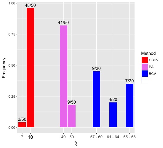
Since (as far as we are aware) our methods for estimating the factor dimension KK and 𝑪\bm{C} are the first methods designed to account for potential correlation among samples, we compared our estimates for KK, 𝑪\bm{C} and subsequently 𝜷\bm{\beta} with state of the art methods designed for data with independent samples. We first evaluated our estimates for KK in 50 simulated datasets in Figure 1 and compared them with the two most widely used methods in the biological literature: parallel analysis (Buja and Eyuboglu, 1992) and bi-cross validation (Owen and Wang, 2016), as implemented in the R-packages SVA (Leek et al., 2017) and CATE (Wang and Zhao, 2015), respectively. As predicted by Theorem 2, our method estimates KK correctly in 48 out of the 50 simulated data sets (Figure 1), while bi-cross validation and parallel analysis drastically overestimate it, since both methods are effectively treating the random effect as part of the latent fixed effect term 𝑳​𝑪⟂T\bm{L}\bm{C}_{\perp}^{T}. We underestimated KK in 2 datasets because the three components with the smallest γk\gamma_{k}’s were shrouded by the heavy-tailed residuals. When residuals were normally distributed, we estimated KK correctly in every dataset.

An interesting feature of Figure 1 is parallel analysis’ estimates for KK are smaller than bi-cross validation’s, which is a manifestation of the more general phenomenon that parallel analysis fails to identify components with smaller eigenvalues γk\gamma_{k} in the presence of components with larger eigenvalues. In fact, when we set γk=n\gamma_{k}=n for k=1,…,5k=1,\ldots,5 and left the remaining eigenvalues as set in Table 1, parallel analysis estimated KK to be only 5. This is because parallel analysis’ approximations of the singular values of 𝒀2\bm{Y}_{2} under the null hypothesis 𝑳​𝑪⟂T=𝟎\bm{L}\bm{C}_{\perp}^{T}=\bm{0} are obtained by independently permuting the entries in each row of 𝒀2\bm{Y}_{2}, and therefore tend to be large when the signal in 𝑳​𝑪⟂T\bm{L}\bm{C}_{\perp}^{T} is large. We refer the reader to Section 3.1 of Dobriban (2017) for a more detailed discussion of this phenomenon.
Refer to caption
Figure 1: Our proposed method’s (CBCV) and parallel analysis’ (PA) estimates for KK in 50 simulated datasets and bi-cross validation’s (BCV) estimates in 20 simulated datasets with the true K=10K=10. We only estimated KK with BCV in 20 datasets because of its slow run time.

Assuming K=10K=10 was known, we next compared the accuracy of our estimates for the column space of 𝑪⟂\bm{C}_{\perp} using ICaSE with the accuracy of KK-partial SVD (Pearson, 1901) and maximum likelihood (Bai and Li, 2012), which first estimates 𝑳\bm{L} and the diagonal matrix 𝚺\bm{\Sigma} under the quasi likelihood model 𝒀2∼M​Np×(n−4)​(𝟎,𝑳​𝑳T+𝚺,In−4)\bm{Y}_{2}\sim MN_{p\times(n-4)}\left(\bm{0},\bm{L}\bm{L}^{T}+\bm{\Sigma},I_{n-4}\right), and sets 𝑪^⟂=𝒀2T​𝚺^−1​𝑳^​(𝑳^T​𝚺^−1​𝑳^)−1\hat{\bm{C}}_{\perp}=\bm{Y}_{2}^{T}\hat{\bm{\Sigma}}^{-1}\hat{\bm{L}}\left(\hat{\bm{L}}^{T}\hat{\bm{\Sigma}}^{-1}\hat{\bm{L}}\right)^{-1}. For each estimate 𝑪^⟂\hat{\bm{C}}_{\perp}, we measured the angle between the column space of 𝑪⟂\bm{C}_{\perp}, Im⁡(𝐂⟂)\im\left(\bm{C}_{\perp}\right), and Im⁡(𝐂^⟂)\im\left(\hat{\bm{C}}_{\perp}\right) as

∡⁡(𝑪⟂,𝑪^⟂)=max𝒗∈Im⁡(𝐂⟂)⁡[min𝒗^∈Im⁡(𝐂^⟂)⁡{cos−1⁡(𝒗^T​𝒗‖𝒗^‖2​‖𝒗‖2)}],\displaystyle\measuredangle\left(\bm{C}_{\perp},\hat{\bm{C}}_{\perp}\right)=\max_{\bm{v}\in\im\left(\bm{C}_{\perp}\right)}\left[\min_{\hat{\bm{v}}\in\im\left(\hat{\bm{C}}_{\perp}\right)}\left\{\cos^{-1}\left(\frac{\hat{\bm{v}}^{T}\bm{v}}{\left\lVert\hat{\bm{v}}\right\rVert_{2}\left\lVert\bm{v}\right\rVert_{2}}\right)\right\}\right],

which is a symmetric function, provided the dimensions of Im⁡(𝐂⟂)\im\left(\bm{C}_{\perp}\right) and Im⁡(𝐂^⟂)\im\left(\hat{\bm{C}}_{\perp}\right) are the same. In order to benchmark the performance of ICaSE, we also simulated additional datasets 𝒀¯∈ℝ15,000×150\bar{\bm{Y}}\in\mathbb{R}^{15,000\times 150} with independent columns, which were generated with the parameters given in (16) and Table 1, except we fixed 𝑽1=⋯=𝑽p=In\bm{V}_{1}=\cdots=\bm{V}_{p}=I_{n}. The angles between the actual and estimated subspace for 50 simulated datasets 𝒀\bm{Y} and 𝒀¯\bar{\bm{Y}} are summarized in Figure 2(a). Just as Theorem 1 predicts and the discussion at the end of Section 3.1 anticipates, ICaSE accurately estimates the column space of 𝑪⟂\bm{C}_{\perp}, whereas naive singular value decomposition and maximum quasi likelihood that ignores the between-sample correlation cannot recover the latent subspace. Further, ICaSE’s estimate for the column space of 𝑪⟂\bm{C}_{\perp} when expression across samples exhibits a complex correlation structure is approximately as accurate as when it is known to be independent.

Refer to caption
(a)
Refer to caption
(b)
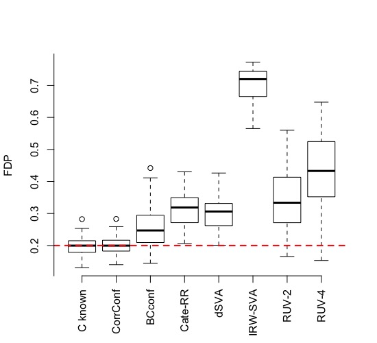
Figure 2: (a): The angle between the actual and estimated 𝑪⟂\bm{C}_{\perp} for 50 simulated datasets 𝒀\bm{Y}, where 𝑪^⟂\hat{\bm{C}}_{\perp} was estimated using our proposed method ICaSE, the first KK right singular vectors of 𝒀2\bm{Y}_{2} (SVD) and maximum quasi likelihood (ML), all with K=10K=10 known. Independent SVD (SVD-Ind) estimated 𝑪⟂\bm{C}_{\perp} as the first K=10K=10 right singular vectors of 𝒀¯2\bar{\bm{Y}}_{2}, which was generated with independent samples. (b): The false discovery proportion (FDP) among genes with a q-value no greater than 0.2 in 50 simulated datasets. We randomly chose 90 genes with βg=0\beta_{g}=0 as control genes in RUV-2 and RUV-4.

We lastly estimated 𝜷\bm{\beta}, the effect of treatment on gene expression in each of the 50 simulated datasets, via generalized least squares with the design matrix 𝑴^=[𝑿​𝒁​𝑪^]\hat{\bm{M}}=\left[\bm{X}\,\bm{Z}\,\hat{\bm{C}}\right], where 𝑪^\hat{\bm{C}} was estimated assuming K=10K=10 was known using CorrConf (our estimator specified in (13)), BCconf (the estimator proposed in McKennan and Nicolae (2018)), Cate-RR (the software default robust regression estimator suggested in Wang et al. (2017)), dSVA (Lee et al., 2017), iteratively re-weighted SVA (IRW-SVA) (Leek and Storey, 2008), RUV-2 (Gagnon-Bartsch and Speed, 2012), RUV-4 (Gagnon-Bartsch et al., 2013) and when 𝑪\bm{C} was known (i.e. 𝑪^=𝑪\hat{\bm{C}}=\bm{C}). In order to make the estimation of 𝑽g\bm{V}_{g} (g=1,…,pg=1,\ldots,p) computationally tractable, we modeled the simulated residuals 𝒆1,…,𝒆p\bm{e}_{1},\ldots,\bm{e}_{p} as

𝒆g∼N⁡(𝟎,vg​𝑽)​(g=1,…,p),𝑽=∑r=13∑s=r3τr​s​𝑩r​s,\displaystyle\bm{e}_{g}\sim N\left(\bm{0},v_{g}\bm{V}\right)\,\,\,(g=1,\ldots,p),\quad\bm{V}=\sum\limits_{r=1}^{3}\sum\limits_{s=r}^{3}\tau_{rs}\bm{B}_{rs},

where 𝑩r​s\bm{B}_{rs} was defined in (17), and estimated v1,…,vpv_{1},\ldots,v_{p} and τr​s\tau_{rs} with restricted maximum likelihood for each of the eight methods using the estimated design matrix 𝑴^\hat{\bm{M}}. We then computed the P value for the null hypothesis βg=0\beta_{g}=0 (g=1,…,pg=1,\ldots,p) by comparing β^g\hat{\beta}_{g} to a t-distribution with n−4−K=n−14n-4-K=n-14 degrees of freedom, used these P values as input into q-value (Storey, 2001) to control the false discovery rate (as this is a software popular among biologists) and deemed a gene to have significantly different expression across the two treatment conditions if its q-value was no greater than 0.2. Figure 2(b) plots the true false discovery proportion in 50 simulated datasets among genes with a q-value less than or equal to 0.2 for each of the eight methods.

The performance of our method (CorrConf), as the statement of Theorem 3 suggests, is nearly indistinguishable from the generalized least squares estimator when 𝑪\bm{C} is known, with nearly identical power. On the other hand, the other six methods tend to introduce more type I errors because their estimates for 𝑪\bm{C} do not account for the dependence between the residuals and therefore fail to recover 𝛀\bm{\Omega}, the variation in 𝑪\bm{C} due to treatment. When KK is underestimated, these six methods have even poorer performance than when K=10K=10 is known, and still fail to control the false discovery rate and exhibit a decrease in power when KK is overestimated to the extent suggested by bi-cross validation and parallel analysis in Figure 1 (see Figure S1 in the Supplement).

The anomalous behavior of IRW-SVA in Figure 2(b) is contingent on the size of 𝛀\bm{\Omega} and the eigenvalues γ1,…,γK\gamma_{1},\ldots,\gamma_{K}. Instead of using the paradigm employed in BCconf, Cate-RR and dSVA of separating 𝜷\bm{\beta} from 𝑳\bm{L} by estimating 𝑳\bm{L} and 𝑪⟂\bm{C}_{\perp} from the residuals 𝒀2\bm{Y}_{2} and 𝛀\bm{\Omega} from 𝑳^\hat{\bm{L}} and 𝒀1\bm{Y}_{1} (with 𝑮=In\bm{G}=I_{n} in (4)), IRW-SVA circumvents estimating 𝛀\bm{\Omega} with the noisy design matrix 𝑳^\hat{\bm{L}} by first identifying the genes with no main effect (i.e. βg=0\beta_{g}=0) and then estimating 𝑪\bm{C} with factor analysis on the reduced data matrix. If KK is known, the proof of Theorem S8.4 in the Supplement suggests that if sufficiently many null genes were correctly identified, 𝛀\bm{\Omega} is sufficiently small, γK\gamma_{K} is sufficiently large and n−1​𝑪T​𝑽∗​𝑪n^{-1}\bm{C}^{T}\bm{V}_{*}\bm{C} is approximately a multiple of n−1​𝑪T​𝑪n^{-1}\bm{C}^{T}\bm{C}, then IRW-SVA can accurately recover 𝑪\bm{C} when samples are correlated. This is not necessarily the case for BCconf, Cate-RR and dSVA, since these methods must additionally use 𝑳^\hat{\bm{L}} to estimate 𝛀\bm{\Omega}, which can be inaccurate depending on the accuracy of 𝑳^\hat{\bm{L}}. However, when both γk\gamma_{k} and the kthk^{\text{th}} column of 𝛀\bm{\Omega} are moderate to large, IRW-SVA attributes a disproportionate amount of the variability in 𝑪\bm{C} as arising from the direct effect of treatment on expression compared to the other three methods. We refer the reader to Section 5.3 of Wang et al. (2017) for a more detailed discussion.

4.3 Modifying existing methods that estimate KK to account for sample correlation

Given the importance of the choice of KK in estimating 𝜷\bm{\beta} and factor analysis in general (Hayton et al., 2004; Brown, 2015; Dobriban, 2017), we discuss three possible adjustments one might suggest to attempt to ameliorate bi-cross validation’s and parallel analysis’ estimates for KK in these simulated data. The simplest would be to merely estimate KK, and subsequently 𝑪\bm{C}, separately for each tissue, since gene expression is assumed to be independent across individuals. If the data within each tissue were sufficiently informative for KK and 𝑪\bm{C}, this procedure should estimate the within-tissue factor dimension to be 10 and 𝑪^t≈𝑪t​𝑹t\hat{\bm{C}}_{t}\approx\bm{C}_{t}\bm{R}_{t} where 𝑪t\bm{C}_{t} is 𝑪\bm{C} restricted to the ttht^{\text{th}} tissue and 𝑹t\bm{R}_{t} is an invertible matrix (t=1,2,3t=1,2,3). The final estimate for KK would then be 3×10=303\times 10=30 and 𝑪^≈𝚷⁡(𝑪1​𝑹1⊕𝑪2​𝑹2⊕𝑪3​𝑹3)\hat{\bm{C}}\approx\bm{\Pi}\left(\bm{C}_{1}\bm{R}_{1}\oplus\bm{C}_{2}\bm{R}_{2}\oplus\bm{C}_{3}\bm{R}_{3}\right), where 𝚷\bm{\Pi} is a permutation matrix that reorders (individual, tissue) pairs. While 𝑪^\hat{\bm{C}} will give approximately unbiased estimates for 𝜷\bm{\beta}, there will be a reduction in the residual degrees of freedom, and therefore power. However, analyzing each tissue separately effectively reduces the sample size (and therefore the eigenvalues γ1,…,γK\gamma_{1},\ldots,\gamma_{K}) by 67% in this simulation example, which is why depending on the analyzed tissue, bi-cross validation and parallel analysis only estimate the within-tissue factor dimension to be anywhere from 1 to 4, which is a marked underestimate of KK.

To discuss the remaining two adjustments, we note that in this simulation example, 𝑽g≈ag​In+bg​𝑩=ag​In+bg​𝒁B​𝒁BT\bm{V}_{g}\approx a_{g}I_{n}+b_{g}\bm{B}=a_{g}I_{n}+b_{g}\bm{Z}_{B}\bm{Z}_{B}^{T}, where 𝑩\bm{B} is a partition matrix that groups the nn samples into n/3n/3 individuals and the columns of 𝒁B∈ℝn×n/3\bm{Z}_{B}\in\mathbb{R}^{n\times n/3} are indicators specifying from which individual the sample originated. The second alteration would be to include 𝒁B\bm{Z}_{B} in the set of nuisance covariates and restrict 𝒀\bm{Y} to the set of 2​n/32n/3 within-individual contrasts. However, this effectively reduces the sample size from nn to 2​n/32n/3 and shrinks the γk\gamma_{k}’s by at least 33%, thereby making it harder to differentiate the latent signal 𝑳​𝑪⟂T\bm{L}\bm{C}_{\perp}^{T} from the noise. In fact, bi-cross validation and parallel analysis had median estimates of KK equal to 8 and 6, respectively, using this alteration. The third adjustment, which avoids dramatically reducing the sample size, is to rotate 𝒀2\bm{Y}_{2} by the eigenvectors of 𝑸[X​Z]T​𝑩​𝑸[X​Z]\bm{Q}_{[X\,Z]}^{T}\bm{B}\bm{Q}_{[X\,Z]}, which in this simulation example shrinks the between-sample dependence but increases the heterogeneity of the sample-specific residual variances. Since parallel analysis only compares the singular values of 𝒀2\bm{Y}_{2} with singular values under a bootstrapped null model, rotating 𝒀2\bm{Y}_{2} did not change parallel analysis’ estimates for KK. On the other hand, bi-cross validation’s estimates for KK should change because cross validation will not be as sensitive to correlations between samples. However, its estimates for 𝑪⟂\bm{C}_{\perp} will still be inaccurate because of the heterogeneity in sample-specific residual variances, which is why its median estimate for KK was only 5 in this simulation example.

5 Sex-specific DNA methylation patterns in a longitudinal twin study

We next applied our method to identify sex-specific DNA methylation patterns from a longitudinal twin study using data previously published in Martino et al. (2013). The authors measured the DNA methylation of 10 monozygotic (MZ) and 5 dizygotic (DZ) Australian twin pairs (all DZ twins were both male or female) at birth and 18 months on the Infinium HumanMethylation450 BeadChip platform in buccal epithelium, a relatively homogeneous tissue. After probe and sample quality filtering and data-normalization, the authors were left with p=330,168p=330,168 methylation sites (CpGs) whose methylation was quantified in 29 male and 24 female (n=53n=53) samples as the difference between log-methylated and log-unmethylated probe intensity (Du et al., 2010) (see Martino et al. (2013) for all pre-processing steps). We then used our proposed method to choose KK and estimate 𝜷\bm{\beta} (CBCV-CorrConf), BCconf, Cate-RR, dSVA and IRW-SVA to identify sex-associated CpGs (CpGs whose methylation differed in males and females), and subsequently validated each method’s findings using sex-associated CpGs identified at birth in previous studies with substantially larger sample sizes. We did not compare our method with RUV-2 or RUV-4, since we did not have access to control CpGs.

We first show that we can write the covariance of the 53 observations at each CpG as a linear combination of six positive semi-definite matrices. Let ym,t,ay_{m,t,a} be the measured DNA methylation for twin t∈{1,2}t\in\left\{1,2\right\}, from mother m∈[15]m\in[15] at age a∈{0,18m}a\in\left\{0,\text{18m}\right\}, where samples with different mothers were assumed to be independent and twin 1 and twin 2 from the same mother were assumed to be exchangeable. A preliminary analysis showed that the correlation between MZ and DZ twins at both ages was approximately the same, which is consistent with the observation that methylation patterns are in large part determined by environmental exposures (Galanter et al., 2017; Martin and Fry, 2018b). Therefore, the 4×44\times 4 covariance matrix for 𝒚m=(ym,1,0​ym,1,18m​ym,2,0​ym,2,18m)T\bm{y}_{m}=\left(y_{m,1,0}\,y_{m,1,\text{18m}}\,y_{m,2,0}\,y_{m,2,\text{18m}}\right)^{T} completely determined the n×nn\times n covariance matrix for each CpG. We avoid assuming a generative model for Cov⁡(𝐲m)\C\left(\bm{y}_{m}\right) by only making assumptions on the pairwise covariances, which averts potential biases in our estimate for 𝑽∗\bm{V}_{*}, and therefore 𝑪\bm{C}. First, we would expect the covariance between observations made on the same individual (or sample) to be at least as large as those made on different individuals (or samples). Second, one might also expect that the shared variance for twins at the same age be as least as large as that at different ages. That is, for a1≠a2a_{1}\neq a_{2} and t1≠t2t_{1}\neq t_{2},

0≤Cov⁡(ym,t1,a1,ym,t2,a2)≤Cov⁡(ym,t1,a1,ym,t1,a2)\displaystyle 0\leq\C\left(y_{m,t_{1},a_{1}},y_{m,t_{2},a_{2}}\right)\leq\C\left(y_{m,t_{1},a_{1}},y_{m,t_{1},a_{2}}\right) ≤Var⁡(ym,t1,ai)​(i=1,2)\displaystyle\leq\V\left(y_{m,t_{1},a_{i}}\right)\,\,\,(i=1,2) (18a)
0≤Cov⁡(ym,t1,a1,ym,t2,a2)≤Cov⁡(ym,t1,ai,ym,t2,ai)\displaystyle 0\leq\C\left(y_{m,t_{1},a_{1}},y_{m,t_{2},a_{2}}\right)\leq\C\left(y_{m,t_{1},a_{i}},y_{m,t_{2},a_{i}}\right) ≤Var⁡(ym,t1,ai)​(i=1,2).\displaystyle\leq\V\left(y_{m,t_{1},a_{i}}\right)\,\,\,(i=1,2). (18b)

Therefore, we can write the covariance matrix for 𝒚m\bm{y}_{m} as

Cov⁡(𝐲m)=\displaystyle\C\left(\bm{y}_{m}\right)= vα​𝟏4​𝟏4T+vη​(𝟏2​𝟏2T⊕𝟏2​𝟏2T)+vϕ,0​𝒂0​𝒂0T+vϕ,18m​𝒂18m​𝒂18mT+v0​diag⁡(𝒂0)+v18m​diag⁡(𝒂18m)\displaystyle v_{\alpha}\bm{1}_{4}\bm{1}_{4}^{T}+v_{\eta}\left(\bm{1}_{2}\bm{1}_{2}^{T}\oplus\bm{1}_{2}\bm{1}_{2}^{T}\right)+v_{\phi,0}\bm{a}_{0}\bm{a}_{0}^{T}+v_{\phi,\text{18m}}\bm{a}_{\text{18m}}\bm{a}_{\text{18m}}^{T}+v_{0}\diag\left(\bm{a}_{0}\right)+v_{\text{18m}}\diag\left(\bm{a}_{\text{18m}}\right)

where 𝒂0T=(1,0,1,0)\bm{a}_{0}^{T}=\left(1,0,1,0\right), 𝒂18mT=(0,1,0,1)\bm{a}_{\text{18m}}^{T}=\left(0,1,0,1\right) and

vα=Cov⁡(ym,t1,0,ym,t2,18m)\displaystyle v_{\alpha}=\C\left(y_{m,t_{1},0},y_{m,t_{2},\text{18m}}\right)
vα+vη=Cov⁡(ym,t1,0,ym,t1,18m),vα+vϕ,a=Cov⁡(ym,t1,a,ym,t2,a)​(a=0,18m)\displaystyle v_{\alpha}+v_{\eta}=\C\left(y_{m,t_{1},0},y_{m,t_{1},\text{18m}}\right),\,\,v_{\alpha}+v_{\phi,a}=\C\left(y_{m,t_{1},a},y_{m,t_{2},a}\right)\,\,\,(a=0,\text{18m})
vα+vη+vϕ,a+va=Var⁡(ym,t1,a)​(a=0,18m).\displaystyle v_{\alpha}+v_{\eta}+v_{\phi,a}+v_{a}=\V\left(y_{m,t_{1},a}\right)\,\,\,(a=0,\text{18m}).

By (18), the variance multipliers also lie in a convex polytope that can be written in the form of (3), and are such that

vα≥0,vη≥0,vϕ,a≥0,vη+va≥0,vϕ,a+va≥0​(a=0,18m),\displaystyle v_{\alpha}\geq 0,\,v_{\eta}\geq 0,\,v_{\phi,a}\geq 0,\,v_{\eta}+v_{a}\geq 0,\,v_{\phi,a}+v_{a}\geq 0\,\,\,(a=0,\text{18m}),

meaning we can apply Algorithm 1 to estimate KK and 𝑪\bm{C} and subsequently identify sex-specific DNA methylation patterns.

Since there was no evidence that the difference in methylation between males and females changed from birth to 18 months, we assumed the methylation at each CpG was a linear combination of the subject’s age (birth or 18 months), sex and other unobserved factors to be estimated, where age was a nuisance covariate and sex was the phenotype of interest. We first used CBCV with F=5F=5 folds and estimated KK to be 2 and then estimated 𝑪\bm{C} and 𝑽∗\bm{V}_{*} with CorrConf. Our estimates for the six average variance multipliers were all strictly greater than 0 and were consistent with previous observations that one’s methylome reflects one’s environmental exposures (Galanter et al., 2017; Martin and Fry, 2018b). That is, the average residual variance at 18 months was 25% larger than that at birth and the correlation between methylation for twins at 18 months was nearly 20% larger than that at birth, indicating this set of twin’s methylomes tended to converge over the first 18 months of life.

We next computed each of the other four method’s estimates for 𝑪\bm{C} using each method’s default software to choose KK: bi-cross validation, the default for Cate-RR and BCconf, or parallel analysis, the default for dSVA and IRW-SVA. Using the full p×np\times n data matrix, bi-cross validation and parallel analysis estimated KK to be 4 and 15, respectively (CBCV also estimated KK to be 4 when we applied it assuming 𝑽g\bm{V}_{g} was a multiple of the identity). The fact that both estimated the latent factor dimension to be greater than CBCV’s estimate of 2 is not surprising, as these methods tend to overestimate KK when samples are correlated. Since these methods are not designed for dependent data and given the complexity of the sample correlation structure for samples from infants with the same mother, we discuss two adjustments designed to alleviate potential biases in their estimates for KK and subsequent test statistics. The first is to split the data matrix into a set of samples measured at birth and another set measured at 18 months, and subsequently rotate the two data matrices to nullify between-twin correlations, which should help to mitigate biases in bi-cross validation’s estimates for K0K_{0} and K18mK_{\text{18m}} (the number of latent factors at birth and 18 months), but leaves parallel analysis’ estimates unchanged. While data splitting removes between-individual correlations, it effectively reduces the sample size by 50% when estimating 𝑪\bm{C} because we are forced to estimate the latent factors at birth and 18 months separately. Bi-cross validation estimated K0=3K_{0}=3, K18m=2K_{\text{18m}}=2 and parallel analysis estimated K0=9K_{0}=9, K18m=7K_{\text{18m}}=7. Lastly, one could split the data by age and twin id into four data matrices, which would ostensibly eliminate the correlation between samples. However, since twin ids are arbitrary, estimates for KK, 𝑪\bm{C} and subsequently 𝜷\bm{\beta} were heavily dependent on how twins were grouped, so we did not include comparisons with this data splitting technique.

Once we estimated 𝑪\bm{C} for all five methods, we estimated the effect due to sex on methylation, and corresponding q-values to control the false discovery rate, exactly as we did for the simulated data in Section 4 and deemed a CpG a sex-associated CpG if its q-value in that method was no greater than 0.2. Since we obviously did not know the ground truth, we used sex-associated CpGs identified at birth in Yousefi et al. (2015) and Maschietto et al. (2017) as a validation set to help judge the veracity of each method’s findings. Yousefi et al. (2015) and Maschietto et al. (2017) measured DNA methylation in umbilical cord blood on the Infinium HumanMethylation450 BeadChip platform in children born to 111 unrelated Brazilian and 71 unrelated Mexican American mothers, respectively. The authors of both studies measured and corrected for cord blood cellular composition and identified 2,355 and 1,928 sex-associated CpGs that were also among the 330,168 CpGs studied in Martino et al. (2013). Table 3 gives the fraction of sex-associated CpGs identified using 𝑪^\hat{\bm{C}} estimated with our method (CBCV-CorrConf), along with the other four methods applied to the full p×np\times n data matrix, that are also among the 3,532 sex-associated CpGs identified in Maschietto et al. (2017) or Yousefi et al. (2015). BCconf’s, Cate-RR’s, dSVA’s and IRW-SVA’s results were nearly identical when we used the data splitting method described in the previous paragraph.

Table 3: The fraction of sex-associated CpGs identified using data from Martino et al. (2013) that are also one of the 3,532 sex-associated CpGs confidently identified in Yousefi et al. (2015) or Maschietto et al. (2017).
CBCV-CorrConf (K=2)(K=2) BCconf (K=4)(K=4) Cate-RR (K=4)(K=4) dSVA (K=15)(K=15) IRW-SVA (K=15)(K=15)
39% (283/735) 23% (424/1836) 20% (474/2404) 19% (487/2513) 28% (341/1236)

While it may be the case that most of BCconf, Cate-RR, dSVA and IRW-SVA are actual sex-associated CpGs, the results in Table 3 mirror the trends observed in Figure 2(b) (as well as those observed in Figure S1 in the Supplement). That is, while these four methods nominally identify more sex-associated CpGs, we are less confident in their results because their estimates for the latent factors reduce the residual variance but likely do not suitably account for the variability in sex explainable by 𝑪\bm{C}, thereby making their results less reproducible.

These results also highlight the importance of the choice of KK. Estimating KK with CBCV (and cross-validation in general) tends to yield more reproducible results because we only include a latent factor if prediction performs suitably well on new, held-out data. When we applied all five methods with K=2K=2, BCconf, Cate-RR and dSVA performed similarly with overlaps no greater than 30% (349 out of dSVA’s 1168 sex-associated CpGs (<30%<30\%) were in the validation set). However, 272 out of IRW-SVA’s 662 sex-associated CpGs (41%) were in the validation set, which is nearly identical to CorrConf’s results in Table 3. Similarly, when we set K=4K=4 for all methods, dSVA performed nearly identically to Cate-RR, whereas CorrConf and IRW-SVA had overlaps of 27% and 26%, respectively, and both ostensibly identified approximately 1,500 sex-associated CpGs. The similarity between CorrConf and IRW-SVA in this dataset is not surprising, since the estimated 𝑪\bm{C}, γK\gamma_{K}, 𝛀\bm{\Omega} and 𝑽∗\bm{V}_{*} satisfied the sufficient conditions for IRW-SVA to accurately recover 𝑪\bm{C} discussed at the end of Section 4.2. We believe K=2K=2 is the most appropriate choice of KK for this dataset because CorrConf’s estimate for 𝑪\bm{C} appears to explain enough of the variance in methylation to achieve reasonable power, while also accurately recovering 𝛀\bm{\Omega} to control for false discoveries and ensuring the results are reproducible.

6 Discussion

To the best of our knowledge, we have provided the first method to account for latent factors in high dimensional data with correlated observations. We proved that our proposed method correlated bi-cross validation (CBCV) tends to accurately choose the latent factor dimension and that our estimate for 𝑪\bm{C} is accurate enough so that asymptotically, inference on the main effect 𝜷\bm{\beta} is just as accurate as when 𝑪\bm{C} is known. We also demonstrated our method’s finite sample properties by analyzing complex, multi-tissue simulated gene expression data, and also used a real longitudinal DNA methylation data from a twin study to show our method tends to give more reproducible results compared to other state of the art methods.

Our proposed procedure is certainly not a panacea for data with arbitrary correlation structure, and relies on the residual variance 𝑽g\bm{V}_{g} being a linear combination of known positive semi-definite matrices. Data with more complex, non-linear sample correlation structure like lengthy auto regressive processes may not be amenable to (2c) without requiring bb to be large, since a linear combination of pp non-linear functions will not necessarily have an apriori known functional form. It may be possible to use the intuition we have developed to first estimate the latent factors with the largest effects, estimate the average unit-specific covariances 𝑽1,…,𝑽p\bm{V}_{1},\ldots,\bm{V}_{p} and use these to subsequently fix 𝑽∗\bm{V}_{*} to approximate KK and 𝑪\bm{C}, since ICaSE, CBCV and (13) only depend on the unit-specific variances through 𝑽∗\bm{V}_{*}. This may be an interesting area of future application.

Another important point is the estimation model we use in (5) is not the only way to approximate the data generating model. In fact, one could argue that 𝒀≈M​Np×n​{𝝁,diag⁡(δ12,⋯,δp2),𝑽}\bm{Y}\approx MN_{p\times n}\left\{\bm{\mu},\diag\left(\delta_{1}^{2},\cdots,\delta_{p}^{2}\right),\bm{V}\right\} is a better approximation to (2). However, ICaSE, and subsequently CBCV, have substantially longer run times with this model (and are intractable with ultra high dimensional DNA methylation data), since we need to repeatedly manipulate and decompose a large p×np\times n matrix as opposed to the relatively small n×nn\times n empirical sample covariance matrix p−1​𝒀T​𝒀p^{-1}\bm{Y}^{T}\bm{Y}. We also did not see any improvement with this model over model (5) in simulations.

7 Software

An R package is available for download at https://github.com/chrismckennan/CorrConf. To install, type the following into the R console:

install.packages("devtools")
devtools::install_github("chrismckennan/CorrConf/CorrConf")
library(CorrConf)

Acknowledgments

We thank Carole Ober and Marcus Soliai for providing data and for comments that have substantially improved the manuscript. This research is supported in part by NIH grants R01-HL129735 and R01-MH101820.

References

  • Agha et al. (2016) Agha, G., Hajj, H., Rifas-Shiman, S. L., Just, A. C., Hivert, M.-F., Burris, H. H., Lin, X., Litonjua, A. A., Oken, E., DeMeo, D. L., Gillman, M. W. and Baccarelli, A. A. (2016) Birth weight-for-gestational age is associated with DNA methylation at birth and in childhood. Clinical Epigenetics, 8, 118.
  • Auffinger and Tang (2015) Auffinger, A. and Tang, S. (2015) Extreme eigenvalues of sparse, heavy tailed random matrices. arXiv:1506.06175v1.
  • Bai and Li (2012) Bai, J. and Li, K. (2012) Statistical analysis of factor models of high dimension. The Annals of Statistics, 40, 436–465.
  • Baumgart et al. (2016) Baumgart, M., Priebe, S., Groth, M., Hartmann, N., Menzel, U., Pandolfini, L., Koch, P., Felder, M., Ristow, M., Englert, C., Guthke, R., Platzer, M. and Cellerino, A. (2016) Longitudinal RNA-Seq analysis of vertebrate aging identifies mitochondrial complex I as a small-molecule-sensitive modifier of lifespan. Cell Systems, 2, 122–132.
  • Breton et al. (2017) Breton, C. V., Marsit, C. J., Faustman, E., Nadeau, K., Goodrich, J. M., Dolinoy, D. C., Herbstman, J., Holland, N., LaSalle, J. M., Schmidt, R., Yousefi, P., Perera, F., Joubert, B. R., Wiemels, J., Taylor, M., Yang, I. V., Chen, R., Hew, K. M., Freeland, D. M. H., Miller, R. and Murphy, S. K. (2017) Small-magnitude effect sizes in epigenetic end points are important in children’s environmental health studies: The children’s environmental health and disease prevention research center’s epigenetics working group. Environmental Health Perspectives, 125, 511–526.
  • Brown (2015) Brown, T. A. (2015) Confirmatory Factor Analysis for Applied Research. Guilford Publications.
  • Buja and Eyuboglu (1992) Buja, A. and Eyuboglu, N. (1992) Remarks on parallel analysis. Multivariate Behavioral Research, 27, 509–540.
  • Carmack et al. (2012) Carmack, P. S., Spence, J. S. and Schucany, W. R. (2012) Generalised correlated cross-validation. Journal of Nonparametric Statistics, 24, 269–282.
  • Dobriban (2017) Dobriban, E. (2017) Factor selection by permutation. arXiv:1710.00479v1.
  • Du et al. (2010) Du, P., Zhang, X., Huang, C.-C., Jafari, N., Kibbe, W. A., Hou, L. and Lin, S. M. (2010) Comparison of beta-value and m-value methods for quantifying methylation levels by microarray analysis. BMC Bioinformatics, 11, 587.
  • Eldar and Kutyniok (2012) Eldar, Y. and Kutyniok, G. (2012) Compressed Sensing: Theory and Applications. Cambridge University Press.
  • Fan and Han (2017) Fan, J. and Han, X. (2017) Estimation of the false discovery proportion with unknown dependence. Journal of the Royal Statistical Society: Series B, 79, 1143–1164.
  • Friedman et al. (2010) Friedman, J., Hastie, T. and Tibshirani, R. (2010) Regularization paths for generalized linear models via coordinate descent. Journal of statistical software, 33, 1–22.
  • Gagnon-Bartsch et al. (2013) Gagnon-Bartsch, J. A., Jacob, L. and Speed, T. P. (2013) Removing unwanted variation from high dimensional data with negative controls. Tech. rep., UC Berkeley.
  • Gagnon-Bartsch and Speed (2012) Gagnon-Bartsch, J. A. and Speed, T. P. (2012) Using control genes to correct for unwanted variation in microarray data. Biostatistics, 13, 539––552.
  • Galanter et al. (2017) Galanter, J. M., Gignoux, C. R., Oh, S. S., Torgerson, D., Pino-Yanes, M., Thakur, N., Eng, C., Hu, D., Huntsman, S., Farber, H. J., Avila, P. C., Brigino-Buenaventura, E., LeNoir, M. A., Meade, K., Serebrisky, D., Rodríguez-Cintrón, W., Kumar, R., Rodríguez-Santana, J. R., Seibold, M. A., Borrell, L. N., Burchard, E. G. and Zaitlen, N. (2017) Differential methylation between ethnic sub-groups reflects the effect of genetic ancestry and environmental exposures. eLife, 6, e20532.
  • Gerard and Carbonetto (2018) Gerard, D. and Carbonetto, P. (2018) vicar: Various Ideas for Confounder Adjustment in Regression.
  • GTEx Consortium (2017) GTEx Consortium (2017) Genetic effects on gene expression across human tissues. Nature, 550.
  • Hastie et al. (2009) Hastie, T., Tibshirani, R. and Friedman, J. (2009) The Elements of Statistical Learning: Data Mining, Inference, and Prediction (Second edition). Springer.
  • Hayton et al. (2004) Hayton, J. C., Allen, D. G. and Scarpello, V. (2004) Factor retention decisions in exploratory factor analysis: a tutorial on parallel analysis. Organizational Research Methods, 7, 191–205.
  • Houseman et al. (2014) Houseman, E. A., Molitor, J. and Marsit, C. J. (2014) Reference-free cell mixture adjustments in analysis of DNA methylation data. Bioinformatics, 30, 1431––1439.
  • Jaffe and Irizarry (2014) Jaffe, A. E. and Irizarry, R. A. (2014) Accounting for cellular heterogeneity is critical in epigenome-wide association studies. Genome Biology, 15.
  • Knowles et al. (2018) Knowles, D. A., Burrows, C. K., Blischak, J. D., Patterson, K. M., Serie, D. J., Norton, N., Ober, C., Pritchard, J. K., Gilad, Y. and McVean, G. (2018) Determining the genetic basis of anthracycline-cardiotoxicity by response QTL mapping in induced cardiomyocytes. eLife, 7, e33480.
  • Lee (2017) Lee, S. (2017) dSVA: Direct Surrogate Variable Analysis.
  • Lee et al. (2017) Lee, S., Sun, W., Wright, F. A. and Zou, F. (2017) An improved and explicit surrogate variable analysis procedure by coefficient adjustment. Biometrika, 104, 303–316.
  • Leek et al. (2017) Leek, J. T., Johnson, W. E., Parker, H. S., Fertig, E. J., Jaffe, A. E., Storey, J. D., Zhang, Y. and Torres, L. C. (2017) sva: Surrogate Variable Analysis. R package version 3.26.0.
  • Leek et al. (2010) Leek, J. T., Scharpf, R. B., Bravo, H. C., Simcha, D., Langmead, B., Johnson, W. E., Geman, D., Baggerly, K. and Irizarry, R. A. (2010) Tackling the widespread and critical impact of batch effects in high-throughput data. Nature reviews. Genetics, 11, 10.1038/nrg2825.
  • Leek and Storey (2008) Leek, J. T. and Storey, J. D. (2008) A general framework for multiple testing dependence. Proceedings of the National Academy of Sciences, 105, 18718–18723.
  • Martin and Fry (2018a) Martin, E. M. and Fry, R. C. (2018a) Environmental influences on the epigenome: Exposure- associated DNA methylation in human populations. Annual Review of Public Health, 39, 309–333.
  • Martin and Fry (2018b) — (2018b) Environmental influences on the epigenome: Exposure- associated DNA methylation in human populations. Annual Review of Public Health, 39, 309–333.
  • Martino et al. (2013) Martino, D., Loke, Y. J., Gordon, L., Ollikainen, M., Cruickshank, M. N., Saffery, R. and Craig, J. M. (2013) Longitudinal, genome-scale analysis of DNA methylation in twins from birth to 18 months of age reveals rapid epigenetic change in early life and pair-specific effects of discordance. Genome Biology, 14, R42.
  • Maschietto et al. (2017) Maschietto, M., Bastos, L. C., Tahira, A. C., Bastos, E. P., Euclydes, V. L. V., Brentani, A., Fink, G., de Baumont, A., Felipe-Silva, A., Francisco, R. P. V., Gouveia, G., Grisi, S. J. F. E., Escobar, A. M. U., Moreira-Filho, C. A., Polanczyk, G. V., Miguel, E. C. and Brentani, H. (2017) Sex differences in DNA methylation of the cord blood are related to sex-bias psychiatric diseases. Scientific Reports, 7.
  • McKennan et al. (2018) McKennan, C., Naughton, K., Stanhope, C., Kattan, M., O’Connor, G., Sandel, M., Visness, C., Wood, R., Bacharier, L., Beigelman, A., Lovisky-Desir, S., Togias, A., Gern, J., Nicolae, D. and Ober, C. (2018) Longitudinal studies at birth and age 7 reveal strong effects of genetic variation on ancestry-associated DNA methylation patterns in blood cells from ethnically admixed children. bioRxiv.
  • McKennan and Nicolae (2018) McKennan, C. and Nicolae, D. (2018) Accounting for unobserved covariates with varying degrees of estimability in high dimensional experimental data. arXiv:1801.00865.
  • Owen and Wang (2016) Owen, A. B. and Wang, J. (2016) Bi-cross-validation for factor analysis. Statistical Science, 31, 119––139.
  • Paul (2007) Paul, D. (2007) Asymptotics of sample eigenstructure for a large dimensional spiked covariance model. Statistica Sinica, 17, 1617–1642.
  • Pearson (1901) Pearson, K. (1901) On Lines and Planes of Closest Fit to Systems of Points in Space. University College.
  • Peixoto et al. (2015) Peixoto, L., Risso, D., Poplawski, S. G., Wimmer, M. E., Speed, T. P., Wood, M. A. and Abel, T. (2015) How data analysis affects power, reproducibility and biological insight of RNA-seq studies in complex datasets. Nucleic Acids Research, 43, 7664–7674.
  • Storey (2001) Storey, J. D. (2001) A direct approach to false discovery rates. Journal of the Royal Statistics Society Series B, 63, 479––498.
  • Sun et al. (2012) Sun, Y., Zhang, N. R. and Owen, A. B. (2012) Multiple hypothesis testing adjusted for latent variables, with an application to the agemap gene expression data. The Annals of Applied Statistics, 6, 1664–1668.
  • Tung et al. (2015) Tung, J., Zhou, X., Alberts, S. C., Stephens, M., Gilad, Y. and Dermitzakis, E. T. (2015) The genetic architecture of gene expression levels in wild baboons. eLife, 4, e04729.
  • Wang and Zhao (2015) Wang, J. and Zhao, Q. (2015) cate: High Dimensional Factor Analysis and Confounder Adjusted Testing and Estimation.
  • Wang et al. (2017) Wang, J., Zhao, Q., Hastie, T. and Owen, A. B. (2017) Confounder adjustment in multiple hypothesis testing. The Annals of Statistics, 45, 1863–1894.
  • Yao et al. (2012) Yao, C., Li, H., Shen, X., He, Z., He, L. and Guo, Z. (2012) Reproducibility and concordance of differential dna methylation and gene expression in cancer. PLOS ONE, 7, e29686–.
  • Yousefi et al. (2015) Yousefi, P., Huen, K., Davé, V., Barcellos, L., Eskenazi, B. and Holland, N. (2015) Sex differences in DNA methylation assessed by 450K beadchip in newborns. BMC Genomics, 16.
  • Yu et al. (2017) Yu, L., Ma, J., Niu, Z., Bai, X., Lei, W., Shao, X., Chen, N., Zhou, F. and Wan, D. (2017) Tissue-specific transcriptome analysis reveals multiple responses to salt stress in populus euphratica seedlings. Genes, 8, 372.

S8 Supplementary Material

S8.1 Additional simulation results

Here we include additional results regarding the estimation of the effect of interest, 𝜷\bm{\beta}, from the simulations discussed in Section 4 when KK is not known to be 10. Since all competing methods perform worse when KK is underestimated, we estimated 𝜷\bm{\beta} using BCconf, Cate-RR, dSVA, IRW-SVA, RUV-2 and RUV-4 in the 50 simulated datasets with K^\hat{K} set to 61, which was the median of all 20 estimates for KK using bi-cross validation. We chose the median bi-cross validation estimate for KK as opposed to the median parallel analysis estimate so that each method had an opportunity to estimate the factors with smallest γk\gamma_{k}’s, which were not recoverable with parallel analysis’ estimate for KK. The results are given in Figure S1, which shows no competing method is able to control for false discovery. Even BCconf, which is the only competing method able to come close to controlling false discovery, has less power than CorrConf to detect true signals. This is presumably because of bi-cross validation’s large estimate of KK, which reduces residual degrees of freedom and increases the estimated variation in 𝑿\bm{X} attributable to 𝑪\bm{C} (i.e. increases 𝛀^\hat{\bm{\Omega}}).

Refer to caption
(a)
Refer to caption
(b)
Figure S1: The false discovery proportion, (a), and true recovery proportion, (b), among genes with a q-value no greater than 0.2 in 50 simulated datasets, where TRP={# of discoveries}/{Total # of genes with βg≠0}\text{TRP}=\left\{\text{\# of discoveries}\right\}/\left\{\text{Total \# of genes with $\beta_{g}\neq 0$}\right\}. The dashed red and blue lines in (a) and (b) are FDP=0.2\text{FDP}=0.2 and TRP={Median TRP when 𝑪 is known}\text{TRP}=\left\{\text{Median TRP when $\bm{C}$ is known}\right\}. We set K^=10\hat{K}=10 in CorrConf (which was CBCV’s median estimate for KK), and K^=61\hat{K}=61 in BCconf, Cate-RR, dSVA, IRW-SVA, RUV-2 and RUV-4.

S8.2 Proofs of all propositions, lemmas and theorems

Unless otherwise stated, we use the notation that a matrix or vector 𝑨=OP​(an)\bm{A}=O_{P}\left(a_{n}\right) if ‖𝑨‖2=OP​(an)\left\lVert\bm{A}\right\rVert_{2}=O_{P}\left(a_{n}\right). We also define

𝑩~j=𝑸XT​𝑩j​𝑸X(j=1,…,b).\displaystyle\tilde{\bm{B}}_{j}=\bm{Q}_{X}^{T}\bm{B}_{j}\bm{Q}_{X}\quad(j=1,\ldots,b).

S8.2.1 Proof of Proposition 1

Proof S8.1 (of Proposition 1).

Since the mean of F(5),(𝛕,δ2)F_{\eqref{equation:WrongModel},\left(\bm{\tau},\delta^{2}\right)} that minimizes the KL divergence is the mean of F(2)F_{\eqref{equation:Model_yANDvar}}, we can write the KL divergence up to constants that do not depend on 𝛕\bm{\tau} or δ2\delta^{2} as

KL{F(2)∣∣F(5),(𝝉,δ2)}=−log|𝒁|+Tr(𝒁𝑽¯)\displaystyle KL\left\{F_{\eqref{equation:Model_yANDvar}}\mid\mid F_{\eqref{equation:WrongModel},\left(\bm{\tau},\delta^{2}\right)}\right\}=-\log\left\lvert\bm{Z}\right\rvert+\Tr\left(\bm{Z}\bar{\bm{V}}\right)

where 𝐙=(δ2​𝐕)−1\bm{Z}=\left(\delta^{2}\bm{V}\right)^{-1} and 𝐕¯=p−1​∑g=1p𝐕g\bar{\bm{V}}=p^{-1}\sum\limits_{g=1}^{p}\bm{V}_{g}. This attains its only minimum when δ∗2​𝐕∗=𝐙∗−1=𝐕¯\delta_{*}^{2}\bm{V}_{*}=\bm{Z}_{*}^{-1}=\bar{\bm{V}}, since the KL-divergence is strictly convex in 𝐙\bm{Z}. We then have

∑j=1bδ∗2τ∗j𝑩j=δ∗2𝑽∗=p−1∑g=1p(∑j=1bvg,j𝑩j)=∑j=1b(p−1∑g=1pvg,j)𝑩j\displaystyle\sum\limits_{j=1}^{b}\delta_{*}^{2}\tau_{*_{j}}\bm{B}_{j}=\delta_{*}^{2}\bm{V}_{*}=p^{-1}\sum\limits_{g=1}^{p}\left(\sum\limits_{j=1}^{b}v_{g,j}\bm{B}_{j}\right)=\sum\limits_{j=1}^{b}\left(p^{-1}\sum\limits_{g=1}^{p}v_{g,j}\right)\bm{B}_{j}

Since the matrix 𝐇\bm{H} defined in the statement of Proposition 1 is positive definite, {vec⁡(𝐁j)}j=1b\left\{\vecM\left(\bm{B}_{j}\right)\right\}_{j=1}^{b} is a linearly independent set, which proves (6). To prove 𝛕∗∈Θ\bm{\tau}_{*}\in\Theta,

𝑨ℐ​𝝉∗=δ∗−2​p−1​∑g=1p𝑨ℐ​𝒗g≥𝟎\displaystyle\bm{A}_{\mathcal{I}}\bm{\tau}_{*}=\delta_{*}^{-2}p^{-1}\sum\limits_{g=1}^{p}\bm{A}_{\mathcal{I}}\bm{v}_{g}\geq\bm{0}

since 𝐀ℐ​𝐯g≥𝟎\bm{A}_{\mathcal{I}}\bm{v}_{g}\geq\bm{0} and

𝑨ℰ​𝝉∗=δ∗−2​p−1​∑g=1p𝑨ℰ​𝒗g=𝟎\displaystyle\bm{A}_{\mathcal{E}}\bm{\tau}_{*}=\delta_{*}^{-2}p^{-1}\sum\limits_{g=1}^{p}\bm{A}_{\mathcal{E}}\bm{v}_{g}=\bm{0}

since 𝐀ℰ​𝐯g=𝟎\bm{A}_{\mathcal{E}}\bm{v}_{g}=\bm{0}. This completes the proof.

S8.2.2 Proof of Theorem 1

We next prove Theorem 1, which will be subsequently used in the proofs of Theorems 2 and 3 and Lemma 1. For ease of notation we will assume in this section that the data 𝒀\bm{Y} are generated according to model (2) with d=0d=0 and will use the incorrect, but simpler model in (5) with d=0d=0 as well in the proofs of Lemma S8.2, Theorem S8.4, Lemma S8.10 and Theorem 1 below. We first prove a lemma about the extreme singular values of a Gaussian random matrix with independent rows.

Lemma S8.2.

Let 𝐄∈ℝp×n\bm{E}\in\mathbb{R}^{p\times n} be a random matrix with independent rows where the gthg^{\text{th}} row is distributed as 𝐞g∼N⁡(0,𝐕g)\bm{e}_{g}\sim N\left(0,\bm{V}_{g}\right) where p−1​∑g=1p𝐕g=𝐕¯p^{-1}\sum\limits_{g=1}^{p}\bm{V}_{g}=\bar{\bm{V}} and suppose Assumption 1 holds. Then

‖p−1𝑬T𝑬−𝑽¯‖2=OP(n1/2p−1/2).\displaystyle\left\lVert p^{-1}\bm{E}^{T}\bm{E}-\bar{\bm{V}}\right\rVert_{2}=O_{P}\left(n^{1/2}p^{-1/2}\right).
Proof S8.3.

The proof of this is a simple extension of Theorem 5.39 in Eldar and Kutyniok (2012) and is omitted.

Theorem S8.4.

Suppose Assumptions 1 and 2 hold and define ϵ=‖𝐕^−𝐕∗‖2\epsilon=\left\lVert\hat{\bm{V}}-\bm{V}_{*}\right\rVert_{2}, where 𝐕^\hat{\bm{V}} is an estimate of 𝐕∗\bm{V}_{*} with log⁡|𝐕^|=0\log\left\lvert\hat{\bm{V}}\right\rvert=0, and

𝑪¯\displaystyle\bar{\bm{C}} =𝑽^−1/2𝑪(𝑪T𝑽^−1𝑪)−1/2\displaystyle=\hat{\bm{V}}^{-1/2}\bm{C}\left(\bm{C}^{T}\hat{\bm{V}}^{-1}\bm{C}\right)^{-1/2} (S1a)
𝑸¯\displaystyle\bar{\bm{Q}} =𝑸𝑪¯\displaystyle=\bm{Q}_{\bar{\bm{C}}} (S1b)
λk\displaystyle\lambda_{k} =𝝀k(p−1𝑽^−1/2𝑪𝑳T𝑳𝑪T𝑽^−1/2).\displaystyle=\bm{\lambda}_{k}\left(p^{-1}\hat{\bm{V}}^{-1/2}\bm{C}\bm{L}^{T}\bm{L}\bm{C}^{T}\hat{\bm{V}}^{-1/2}\right). (S1c)

where 𝛌k​(𝐀)\bm{\lambda}_{k}\left(\bm{A}\right) is the kthk^{\text{th}} largest eigenvector of the matrix 𝐀\bm{A}. Define the estimates 𝐂¯^∈ℝn×K\hat{\bar{\bm{C}}}\in\mathbb{R}^{n\times K} and λ^1,…,λ^K\hat{\lambda}_{1},\ldots,\hat{\lambda}_{K} to be the first KK eigenvectors and eigenvalues of 𝐕^−1/2p−1𝐘T𝐘𝐕^−1/2\hat{\bm{V}}^{-1/2}p^{-1}\bm{Y}^{T}\bm{Y}\hat{\bm{V}}^{-1/2}, respectively. Then if ϵ/γK=oP​(1)\epsilon/\gamma_{K}=o_{P}(1),

‖P𝑪¯−P𝑪¯^‖F2\displaystyle\left\lVert P_{\bar{\bm{C}}}-P_{\hat{\bar{\bm{C}}}}\right\rVert_{F}^{2} =OP[{n1/2(γKp)−1/2+ϵγK−1}2].\displaystyle=O_{P}\left[\left\{n^{1/2}\left(\gamma_{K}p\right)^{-1/2}+\epsilon\gamma_{K}^{-1}\right\}^{2}\right]. (S2)

Further, if ϵ=oP​(1)\epsilon=o_{P}(1),

λ^k/λk=1+δ∗2/λk+OP{n(γKp)−1+n1/2(γKp)−1/2ϵ+(γKp)−1/2+ϵγK−1}\displaystyle\hat{\lambda}_{k}/\lambda_{k}=1+\delta_{*}^{2}/\lambda_{k}+O_{P}\left\{n\left(\gamma_{K}p\right)^{-1}+n^{1/2}\left(\gamma_{K}p\right)^{-1/2}\epsilon+\left(\gamma_{K}p\right)^{-1/2}+\epsilon\gamma_{K}^{-1}\right\} (S3)
‖𝑪¯T𝑪¯^−IK‖2=OP{n(γKp)−1+n1/2(γKp)−1/2ϵ+(γKp)−1/2+ϵγK−1}.\displaystyle\left\lVert\bar{\bm{C}}^{T}\hat{\bar{\bm{C}}}-I_{K}\right\rVert_{2}=O_{P}\left\{n\left(\gamma_{K}p\right)^{-1}+n^{1/2}\left(\gamma_{K}p\right)^{-1/2}\epsilon+\left(\gamma_{K}p\right)^{-1/2}+\epsilon\gamma_{K}^{-1}\right\}. (S4)
Proof S8.5.

First, (λk−λk+1)/λk+1≥c1−1+oP​(1)(\lambda_{k}-\lambda_{k+1})/\lambda_{k+1}\geq c_{1}^{-1}+o_{P}(1) when ϵ=oP​(1)\epsilon=o_{P}(1) by item (a) of Assumption 1. Next, since 𝐋\bm{L} and 𝐂\bm{C} are unique up to a K×KK\times K invertible matrix, it suffices to re-define 𝐋\bm{L} as 𝐋(n−1𝐂T𝐕^−1𝐂)+1/2\bm{L}\left(n^{-1}\bm{C}^{T}\hat{\bm{V}}^{-1}\bm{C}\right)^{+1/2} and assume n​p−1​𝐋T​𝐋=diag⁡(λ1,…,λK)np^{-1}\bm{L}^{T}\bm{L}=\diag\left(\lambda_{1},\ldots,\lambda_{K}\right). We let γ=γK\gamma=\gamma_{K} and use a technique developed in Paul (2007) and define the rotated matrix 𝐒¯\bar{\bm{S}} to be

𝑺¯\displaystyle\bar{\bm{S}} =(𝑪¯T𝑸¯T)(γp)−1𝑽^−1/2𝒀T𝒀𝑽^−1/2(𝑪¯𝑸¯)={(𝑳¯+𝑬¯1)T​(𝑳¯+𝑬¯1)(𝑳¯+𝑬¯1)T​𝑬¯2𝑬¯2T​(𝑳¯+𝑬¯1)𝑬¯2T​𝑬¯2}\displaystyle=\begin{pmatrix}\bar{\bm{C}}^{T}\\ \bar{\bm{Q}}^{T}\end{pmatrix}\left(\gamma p\right)^{-1}\hat{\bm{V}}^{-1/2}\bm{Y}^{T}\bm{Y}\hat{\bm{V}}^{-1/2}\begin{pmatrix}\bar{\bm{C}}&\bar{\bm{Q}}\end{pmatrix}=\left\{\begin{matrix}\left(\bar{\bm{L}}+\bar{\bm{E}}_{1}\right)^{T}\left(\bar{\bm{L}}+\bar{\bm{E}}_{1}\right)&\left(\bar{\bm{L}}+\bar{\bm{E}}_{1}\right)^{T}\bar{\bm{E}}_{2}\\ \bar{\bm{E}}_{2}^{T}\left(\bar{\bm{L}}+\bar{\bm{E}}_{1}\right)&\bar{\bm{E}}_{2}^{T}\bar{\bm{E}}_{2}\end{matrix}\right\} (S5)
𝑳¯\displaystyle\bar{\bm{L}} =n1/2(γp)−1/2𝑳\displaystyle=n^{1/2}\left(\gamma p\right)^{-1/2}\bm{L} (S6)
𝑬¯1\displaystyle\bar{\bm{E}}_{1} =(γp)−1/2𝑬𝑽^−1/2𝑪¯\displaystyle=\left(\gamma p\right)^{-1/2}\bm{E}\hat{\bm{V}}^{-1/2}\bar{\bm{C}} (S7)
𝑬¯2\displaystyle\bar{\bm{E}}_{2} =(γp)−1/2𝑬𝑽^−1/2𝑸¯.\displaystyle=\left(\gamma p\right)^{-1/2}\bm{E}\hat{\bm{V}}^{-1/2}\bar{\bm{Q}}. (S8)

We now get explicit error bounds for terms in 𝐒¯\bar{\bm{S}}.

  1. 1.
    𝑳¯T​𝑬¯1\displaystyle\bar{\bm{L}}^{T}\bar{\bm{E}}_{1} =(γp)−1/2𝑳¯T𝑬𝑽^−1(n−1/2𝑪)(n−1𝑪T𝑽^−1𝑪)−1/2⏟OP​(1)\displaystyle=\left(\gamma p\right)^{-1/2}\bar{\bm{L}}^{T}\bm{E}\hat{\bm{V}}^{-1}\left(n^{-1/2}\bm{C}\right)\underbrace{\left(n^{-1}\bm{C}^{T}\hat{\bm{V}}^{-1}\bm{C}\right)^{-1/2}}_{O_{P}(1)}
    =((γp)−1/2𝑳¯T𝑬𝑽−1∗(n−1/2𝑪)⏟OP{(γp)−1/2}+(γp)−1/2𝑳¯T𝑬(𝑽^−1−𝑽−1∗)(n−1/2𝑪)⏟OP{n1/2(γp)−1/2ϵ})OP(1).\displaystyle=\left(\underbrace{\left(\gamma p\right)^{-1/2}\bar{\bm{L}}^{T}\bm{E}\bm{V}^{-1}_{*}\left(n^{-1/2}\bm{C}\right)}_{O_{P}\left\{\left(\gamma p\right)^{-1/2}\right\}}+\underbrace{\left(\gamma p\right)^{-1/2}\bar{\bm{L}}^{T}\bm{E}\left(\hat{\bm{V}}^{-1}-\bm{V}^{-1}_{*}\right)\left(n^{-1/2}\bm{C}\right)}_{O_{P}\left\{n^{1/2}\left(\gamma p\right)^{-1/2}\epsilon\right\}}\right)O_{P}(1).

    Therefore, ‖𝑳¯T𝑬¯1‖2=OP{(γp)−1/2+n1/2(γp)−1/2ϵ}\left\lVert\bar{\bm{L}}^{T}\bar{\bm{E}}_{1}\right\rVert_{2}=O_{P}\left\{\left(\gamma p\right)^{-1/2}+n^{1/2}\left(\gamma p\right)^{-1/2}\epsilon\right\}.

  2. 2.
    𝑳¯T​𝑬¯2\displaystyle\bar{\bm{L}}^{T}\bar{\bm{E}}_{2} =(γp)−1/2𝑳¯T𝑬𝑽^−1/2𝑽^1/2𝑸𝑪⏟OP{n1/2(γp)−1/2}(𝑸𝑪T𝑽^𝑸𝑪)−1/2⏟OP​(1).\displaystyle=\underbrace{\left(\gamma p\right)^{-1/2}\bar{\bm{L}}^{T}\bm{E}\hat{\bm{V}}^{-1/2}\hat{\bm{V}}^{1/2}\bm{Q}_{\bm{C}}}_{O_{P}\left\{n^{1/2}\left(\gamma p\right)^{-1/2}\right\}}\underbrace{\left(\bm{Q}_{\bm{C}}^{T}\hat{\bm{V}}\bm{Q}_{\bm{C}}\right)^{-1/2}}_{O_{P}(1)}.

    Therefore, ‖𝑳¯T𝑬¯2‖2=OP{n1/2(γp)−1/2}\left\lVert\bar{\bm{L}}^{T}\bar{\bm{E}}_{2}\right\rVert_{2}=O_{P}\left\{n^{1/2}\left(\gamma p\right)^{-1/2}\right\}.

  3. 3.
    𝑬¯1T𝑬¯1=(γp)−1𝑪¯T𝑽∗−1/2𝑬T𝑬𝑽∗−1/2𝑪¯+OP(ϵγ−1).\displaystyle\bar{\bm{E}}_{1}^{T}\bar{\bm{E}}_{1}=\left(\gamma p\right)^{-1}\bar{\bm{C}}^{T}\bm{V}^{-1/2}_{*}\bm{E}^{T}\bm{E}\bm{V}^{-1/2}_{*}\bar{\bm{C}}+O_{P}\left(\epsilon\gamma^{-1}\right).

    Define 𝑪~=𝑽∗−1/2𝑪(𝑪T𝑽∗−1𝑪)−1/2\tilde{\bm{C}}=\bm{V}^{-1/2}_{*}\bm{C}\left(\bm{C}^{T}\bm{V}^{-1}_{*}\bm{C}\right)^{-1/2}.

    (γp)−1𝑪¯T𝑽^−1/2𝑬T𝑬𝑽^−1/2𝑪¯\displaystyle\left(\gamma p\right)^{-1}\bar{\bm{C}}^{T}\hat{\bm{V}}^{-1/2}\bm{E}^{T}\bm{E}\hat{\bm{V}}^{-1/2}\bar{\bm{C}} =γ−1δ∗2IK+γ−1𝑪¯T(𝑽^−1/2p−1𝑬T𝑬𝑽^−1/2−δ∗2In)𝑪¯\displaystyle=\gamma^{-1}\delta_{*}^{2}I_{K}+\gamma^{-1}\bar{\bm{C}}^{T}\left(\hat{\bm{V}}^{-1/2}p^{-1}\bm{E}^{T}\bm{E}\hat{\bm{V}}^{-1/2}-\delta_{*}^{2}I_{n}\right)\bar{\bm{C}}
    =γ−1δ∗2IK+γ−1𝑪~T(𝑽−1/2∗p−1𝑬T𝑬𝑽−1/2∗−δ∗2In)𝑪~⏟OP(γ−1p−1/2)+OP(ϵγ−1).\displaystyle=\gamma^{-1}\delta_{*}^{2}I_{K}+\underbrace{\gamma^{-1}\tilde{\bm{C}}^{T}\left(\bm{V}^{-1/2}_{*}p^{-1}\bm{E}^{T}\bm{E}\bm{V}^{-1/2}_{*}-\delta_{*}^{2}I_{n}\right)\tilde{\bm{C}}}_{O_{P}\left(\gamma^{-1}p^{-1/2}\right)}+O_{P}\left(\epsilon\gamma^{-1}\right).

    Therefore,

    ‖𝑬¯1T𝑬¯1−γ−1δ∗2IK‖2=OP(ϵγ−1+γ−1p−1/2).\displaystyle\left\lVert\bar{\bm{E}}_{1}^{T}\bar{\bm{E}}_{1}-\gamma^{-1}\delta_{*}^{2}I_{K}\right\rVert_{2}=O_{P}\left(\epsilon\gamma^{-1}+\gamma^{-1}p^{-1/2}\right).
  4. 4.

    Let 𝑸~=𝑸𝑪~\tilde{\bm{Q}}=\bm{Q}_{\tilde{\bm{C}}}. Then

    𝑬¯1T𝑬¯2=(γp)−1𝑪¯T𝑽^−1/2𝑬T𝑬𝑽^−1/2𝑸¯=(γp)−1𝑪~T𝑽∗−1/2𝑬T𝑬𝑽∗−1/2𝑸~+OP(ϵγ−1).\displaystyle\bar{\bm{E}}_{1}^{T}\bar{\bm{E}}_{2}=\left(\gamma p\right)^{-1}\bar{\bm{C}}^{T}\hat{\bm{V}}^{-1/2}\bm{E}^{T}\bm{E}\hat{\bm{V}}^{-1/2}\bar{\bm{Q}}=\left(\gamma p\right)^{-1}\tilde{\bm{C}}^{T}\bm{V}^{-1/2}_{*}\bm{E}^{T}\bm{E}\bm{V}^{-1/2}_{*}\tilde{\bm{Q}}+O_{P}\left(\epsilon\gamma^{-1}\right).

    Let 𝑬~=p−1/2𝑬𝑽−1/2∗,𝑬~1=𝑬~𝑪~,𝑬~2=𝑬~𝑸~\tilde{\bm{E}}=p^{-1/2}\bm{E}\bm{V}^{-1/2}_{*},\tilde{\bm{E}}_{1}=\tilde{\bm{E}}\tilde{\bm{C}},\tilde{\bm{E}}_{2}=\tilde{\bm{E}}\tilde{\bm{Q}} and 𝑨g=𝑽−1/2∗𝑽g𝑽−1/2∗\bm{A}_{g}=\bm{V}^{-1/2}_{*}\bm{V}_{g}\bm{V}^{-1/2}_{*}. Then the kthk^{\text{th}} column of 𝑬~2T​𝑬~1\tilde{\bm{E}}_{2}^{T}\tilde{\bm{E}}_{1} (k=1,…,Kk=1,\ldots,K) is

    𝒃k\displaystyle\bm{b}_{k} =p−1​𝑸~T​𝑬~T​𝑬~​𝒄~k=𝑸~T​(p−1​𝑬~T​𝑬~−p−1​∑g=1p𝑨g)​𝒄~k+𝑸~T​p−1​∑g=1p𝑨g⏟=δ∗2​In​𝒄~k\displaystyle=p^{-1}\tilde{\bm{Q}}^{T}\tilde{\bm{E}}^{T}\tilde{\bm{E}}\tilde{\bm{c}}_{k}=\tilde{\bm{Q}}^{T}\left(p^{-1}\tilde{\bm{E}}^{T}\tilde{\bm{E}}-p^{-1}\sum\limits_{g=1}^{p}\bm{A}_{g}\right)\tilde{\bm{c}}_{k}+\tilde{\bm{Q}}^{T}\underbrace{p^{-1}\sum\limits_{g=1}^{p}\bm{A}_{g}}_{=\delta_{*}^{2}I_{n}}\tilde{\bm{c}}_{k}
    =p−1​∑g=1p𝑸~T​𝑨g1/2​(𝒓g​𝒓gT−δ∗2​In)​𝑨g1/2​𝒄~k=p−1​∑g=1p𝒃g,k\displaystyle=p^{-1}\sum\limits_{g=1}^{p}\tilde{\bm{Q}}^{T}\bm{A}_{g}^{1/2}\left(\bm{r}_{g}\bm{r}_{g}^{T}-\delta_{*}^{2}I_{n}\right)\bm{A}_{g}^{1/2}\tilde{\bm{c}}_{k}=p^{-1}\sum\limits_{g=1}^{p}\bm{b}_{g,k}

    where 𝒓g∼N⁡(𝟎,In)\bm{r}_{g}\sim N\left(\bm{0},I_{n}\right), 𝒓g\bm{r}_{g} and 𝒓g′\bm{r}_{g^{\prime}} are independent for g≠g′g\neq g^{\prime} (g=1,…,p;g′=1,…,pg=1,\ldots,p;g^{\prime}=1,\ldots,p) and 𝔼⁡(𝐛k)=𝟎\E\left(\bm{b}_{k}\right)=\bm{0}. Therefore,

    𝔼⁡(‖𝐛k‖22)=∑i=1n−K𝔼⁡(𝐛ki2)=∑i=1n−KVar⁡(𝐛ki)=O⁡{n​Var⁡(𝐛k1)}=O⁡(np−1)\displaystyle\E\left(\left\lVert\bm{b}_{k}\right\rVert_{2}^{2}\right)=\sum\limits_{i=1}^{n-K}\E\left(\bm{b}_{ki}^{2}\right)=\sum\limits_{i=1}^{n-K}\V\left(\bm{b}_{ki}\right)=O\left\{n\V\left(\bm{b}_{k1}\right)\right\}=O\left(np^{-1}\right)

    where the second to last and last equalities follow because ‖𝑨g‖2\left\lVert\bm{A}_{g}\right\rVert_{2} is uniformly bounded by item (a) of Assumption 1. Therefore, ‖𝑬¯2T𝑬¯1‖2=OP(γ−1n1/2p−1/2+ϵγ−1)\left\lVert\bar{\bm{E}}_{2}^{T}\bar{\bm{E}}_{1}\right\rVert_{2}=O_{P}\left(\gamma^{-1}n^{1/2}p^{-1/2}+\epsilon\gamma^{-1}\right).

Let μk=λk/γ\mu_{k}=\lambda_{k}/\gamma and define (𝐯^kT𝐳^kT)T∈ℝn\begin{pmatrix}\hat{\bm{v}}_{k}^{T}&\hat{\bm{z}}_{k}^{T}\end{pmatrix}^{T}\in\mathbb{R}^{n} to be the kthk^{\text{th}} normalized eigenvector of 𝐒¯\bar{\bm{S}}, where 𝐯k∈ℝK\bm{v}_{k}\in\mathbb{R}^{K} and 𝐳k∈ℝn−K\bm{z}_{k}\in\mathbb{R}^{n-K}. All of this proves that μ^k=μk+δ∗2/γ+oP​(1)\hat{\mu}_{k}=\mu_{k}+\delta_{*}^{2}/\gamma+o_{P}(1) by Weyl’s theorem. To prove sharper bounds, we set set up the eigenvalue equations

μ^k​𝒗^k\displaystyle\hat{\mu}_{k}\hat{\bm{v}}_{k} =(𝑳¯+𝑬¯1)T​(𝑳¯+𝑬¯1)​𝒗^k+(𝑳¯+𝑬¯1)T​𝑬¯2​𝒛^k\displaystyle=\left(\bar{\bm{L}}+\bar{\bm{E}}_{1}\right)^{T}\left(\bar{\bm{L}}+\bar{\bm{E}}_{1}\right)\hat{\bm{v}}_{k}+\left(\bar{\bm{L}}+\bar{\bm{E}}_{1}\right)^{T}\bar{\bm{E}}_{2}\hat{\bm{z}}_{k}
μ^k​𝒛k\displaystyle\hat{\mu}_{k}\bm{z}_{k} =𝑬¯2T​(𝑳¯+𝑬¯1)​𝒗^k+𝑬¯2T​𝑬¯2​𝒛^k.\displaystyle=\bar{\bm{E}}_{2}^{T}\left(\bar{\bm{L}}+\bar{\bm{E}}_{1}\right)\hat{\bm{v}}_{k}+\bar{\bm{E}}_{2}^{T}\bar{\bm{E}}_{2}\hat{\bm{z}}_{k}.

A little algebra shows that

μ^k​𝒗^k\displaystyle\hat{\mu}_{k}\hat{\bm{v}}_{k} ={(𝑳¯+𝑬¯1)T​(𝑳¯+𝑬¯1)+(𝑳¯+𝑬¯1)T​𝑬¯2​(μ^k​In−𝑬¯2T​𝑬¯2)−1​𝑬¯2T​(𝑳¯+𝑬¯1)}​𝒗^k\displaystyle=\left\{\left(\bar{\bm{L}}+\bar{\bm{E}}_{1}\right)^{T}\left(\bar{\bm{L}}+\bar{\bm{E}}_{1}\right)+\left(\bar{\bm{L}}+\bar{\bm{E}}_{1}\right)^{T}\bar{\bm{E}}_{2}\left(\hat{\mu}_{k}I_{n}-\bar{\bm{E}}_{2}^{T}\bar{\bm{E}}_{2}\right)^{-1}\bar{\bm{E}}_{2}^{T}\left(\bar{\bm{L}}+\bar{\bm{E}}_{1}\right)\right\}\hat{\bm{v}}_{k} (S9)
𝒛^k\displaystyle\hat{\bm{z}}_{k} =(μ^k​In−𝑬¯2T​𝑬¯2)−1​𝑬¯2T​(𝑳¯+𝑬¯1)​𝒗^k\displaystyle=\left(\hat{\mu}_{k}I_{n}-\bar{\bm{E}}_{2}^{T}\bar{\bm{E}}_{2}\right)^{-1}\bar{\bm{E}}_{2}^{T}\left(\bar{\bm{L}}+\bar{\bm{E}}_{1}\right)\hat{\bm{v}}_{k} (S10)

where μ^k​In−𝐄¯2T​𝐄¯2\hat{\mu}_{k}I_{n}-\bar{\bm{E}}_{2}^{T}\bar{\bm{E}}_{2} is invertible because μ^k=μk+δ∗2/γ+oP​(1)\hat{\mu}_{k}=\mu_{k}+\delta_{*}^{2}/\gamma+o_{P}(1) and by Lemma S8.2. By what we showed above, we then have that

‖𝒛^k‖2\displaystyle\left\lVert\hat{\bm{z}}_{k}\right\rVert_{2} =OP{n1/2(γp)−1/2+ϵγ−1}\displaystyle=O_{P}\left\{n^{1/2}\left(\gamma p\right)^{-1/2}+\epsilon\gamma^{-1}\right\} (S11a)
μ^k\displaystyle\hat{\mu}_{k} =𝝀k{(𝑳¯+𝑬¯1)T(𝑳¯+𝑬¯1)}+OP[{n1/2(γp)−1/2+ϵγ−1}2]\displaystyle=\bm{\lambda}_{k}\left\{\left(\bar{\bm{L}}+\bar{\bm{E}}_{1}\right)^{T}\left(\bar{\bm{L}}+\bar{\bm{E}}_{1}\right)\right\}+O_{P}\left[\left\{n^{1/2}\left(\gamma p\right)^{-1/2}+\epsilon\gamma^{-1}\right\}^{2}\right]
=μk+δ∗2γ−1+OP{n(γp)−1+n1/2(γp)−1/2ϵ+(γp)−1/2+ϵγ−1}\displaystyle=\mu_{k}+\delta_{*}^{2}\gamma^{-1}+O_{P}\left\{n\left(\gamma p\right)^{-1}+n^{1/2}\left(\gamma p\right)^{-1/2}\epsilon+\left(\gamma p\right)^{-1/2}+\epsilon\gamma^{-1}\right\} (S11b)
‖𝒗^k−𝒗k‖2\displaystyle\left\lVert\hat{\bm{v}}_{k}-\bm{v}_{k}\right\rVert_{2} =OP[{n1/2(γp)−1/2+ϵγ−1}2]\displaystyle=O_{P}\left[\left\{n^{1/2}\left(\gamma p\right)^{-1/2}+\epsilon\gamma^{-1}\right\}^{2}\right] (S11c)
‖𝒗^k−𝒂k‖2\displaystyle\left\lVert\hat{\bm{v}}_{k}-\bm{a}_{k}\right\rVert_{2} =OP{n(γp)−1+n1/2(γp)−1/2ϵ+(γp)−1/2+ϵγ−1}\displaystyle=O_{P}\left\{n\left(\gamma p\right)^{-1}+n^{1/2}\left(\gamma p\right)^{-1/2}\epsilon+\left(\gamma p\right)^{-1/2}+\epsilon\gamma^{-1}\right\} (S11d)

where 𝐯k\bm{v}_{k} is the kthk^{\text{th}} eigenvector of (𝐋¯+𝐄¯1)T​(𝐋¯+𝐄¯1)\left(\bar{\bm{L}}+\bar{\bm{E}}_{1}\right)^{T}\left(\bar{\bm{L}}+\bar{\bm{E}}_{1}\right) and 𝐚k∈ℝK\bm{a}_{k}\in\mathbb{R}^{K} is the kthk^{\text{th}} standard basis vector. Equation (S11a) follow from Weyl’s Theorem (i.e. μ^k=μk+δ∗2/λk+oP​(1)\hat{\mu}_{k}=\mu_{k}+\delta_{*}^{2}/\lambda_{k}+o_{P}(1)) and (S11b) follows from Theorem 3.5 of Auffinger and Tang (2015) and the assumption that (λk−λk+1)/λk+1≥c1−1+oP​(1)(\lambda_{k}-\lambda_{k+1})/\lambda_{k+1}\geq c_{1}^{-1}+o_{P}(1). Since the left and right singular vectors of any matrix are unique up to sign parity, a second application of Theorem 3.5 of Auffinger and Tang (2015), along with the assumption that (λk−λk+1)/λk+1≥c1−1+oP​(1)(\lambda_{k}-\lambda_{k+1})/\lambda_{k+1}\geq c_{1}^{-1}+o_{P}(1), proves (S11c) and (S11d). This proves (S3).

Define 𝒗^=(𝒗^1⋯𝒗^K)\hat{\bm{v}}=\begin{pmatrix}\hat{\bm{v}}_{1}&\cdots&\hat{\bm{v}}_{K}\end{pmatrix} and 𝒛^=(𝒛^1⋯𝒛^K)\hat{\bm{z}}=\begin{pmatrix}\hat{\bm{z}}_{1}&\cdots&\hat{\bm{z}}_{K}\end{pmatrix}. Since 𝒗^T​𝒗^+𝒛^T​𝒛^=IK\hat{\bm{v}}^{T}\hat{\bm{v}}+\hat{\bm{z}}^{T}\hat{\bm{z}}=I_{K} and by (S11a),

‖𝒗^𝒗^T−IK‖2=OP[{n1/2(γp)−1/2+ϵγ−1}2].\displaystyle\left\lVert\hat{\bm{v}}\hat{\bm{v}}^{T}-I_{K}\right\rVert_{2}=O_{P}\left[\left\{n^{1/2}\left(\gamma p\right)^{-1/2}+\epsilon\gamma^{-1}\right\}^{2}\right].

Then

𝑪¯^=𝑪¯​𝒗^+𝑸¯​𝒛^\displaystyle\hat{\bar{\bm{C}}}=\bar{\bm{C}}\hat{\bm{v}}+\bar{\bm{Q}}\hat{\bm{z}} (S12)

with

‖P𝑪¯^−P𝑪¯‖F2=2K−2Tr[𝑪¯T𝑪¯^𝑪¯^T𝑪¯]=2K−2Tr[𝒗^𝒗^T]=OP[{n1/2(γp)−1/2+ϵγ−1}2],\displaystyle\left\lVert P_{\hat{\bar{\bm{C}}}}-P_{\bar{\bm{C}}}\right\rVert_{F}^{2}=2K-2\Tr\left[\bar{\bm{C}}^{T}\hat{\bar{\bm{C}}}\hat{\bar{\bm{C}}}^{T}\bar{\bm{C}}\right]=2K-2\Tr\left[\hat{\bm{v}}\hat{\bm{v}}^{T}\right]=O_{P}\left[\left\{n^{1/2}\left(\gamma p\right)^{-1/2}+\epsilon\gamma^{-1}\right\}^{2}\right],

which proves (S2). Lastly, (S4) follows from (S11c) and (S11d).

We note that because δ^2​𝝉^∈Θ∗\hat{\delta}^{2}\hat{\bm{\tau}}\in\Theta_{*} by Assumption 2, we may assume that (n−d)−1​𝑪⟂T​𝑾^−1​𝑪⟂=In−K(n-d)^{-1}\bm{C}_{\perp}^{T}\hat{\bm{W}}^{-1}\bm{C}_{\perp}=I_{n-K}, (n−d)​p−1​𝑳T​𝑳=diag⁡(λ1,…,λK)(n-d)p^{-1}\bm{L}^{T}\bm{L}=\diag\left(\lambda_{1},\ldots,\lambda_{K}\right) where λK≤⋯≤λ1\lambda_{K}\leq\cdots\leq\lambda_{1} and λ1,λK≍γK\lambda_{1},\lambda_{K}\asymp\gamma_{K} for any fixed estimates δ^2,𝝉^\hat{\delta}^{2},\hat{\bm{\tau}} in the proofs of Theorems 1, 2 and 3 because the statement of those theorems only involves the columns space of 𝑪\bm{C}. Since we will eventually prove (7a) in Theorem 1 when KK is known and

n1/2​‖(n−d)−1​𝑪⟂T​𝑾∗−1​𝑪⟂−(n−d)−1​𝑪⟂T​𝑾^∗−1​𝑪⟂‖2=oP​(1),\displaystyle n^{1/2}\left\lVert(n-d)^{-1}\bm{C}_{\perp}^{T}\bm{W}_{*}^{-1}\bm{C}_{\perp}-(n-d)^{-1}\bm{C}_{\perp}^{T}\hat{\bm{W}}_{*}^{-1}\bm{C}_{\perp}\right\rVert_{2}=o_{P}(1),
n1/2​‖𝛀​{(n−d)−1​𝑪⟂T​𝑾^∗−1​𝑪⟂}1/2−𝛀‖2=oP​(1).\displaystyle n^{1/2}\left\lVert\bm{\Omega}\left\{(n-d)^{-1}\bm{C}_{\perp}^{T}\hat{\bm{W}}_{*}^{-1}\bm{C}_{\perp}\right\}^{1/2}-\bm{\Omega}\right\rVert_{2}=o_{P}(1).

Therefore, we assume (n−d)−1​𝑪⟂T​𝑾^−1​𝑪⟂=In−K(n-d)^{-1}\bm{C}_{\perp}^{T}\hat{\bm{W}}^{-1}\bm{C}_{\perp}=I_{n-K} and (n−d)​p−1​𝑳T​𝑳(n-d)p^{-1}\bm{L}^{T}\bm{L} is diagonal with decreasing elements in the remainder of the supplement, including the proof of Lemma 1.

Corollary S8.6 (used in the proof of Theorems 1 and 3).

Suppose the assumptions of Theorem S8.4 hold (including the assumption that ϵ=oP​(1)\epsilon=o_{P}(1)) and let 𝐌g∈ℝn×n\bm{M}_{g}\in\mathbb{R}^{n\times n} be a random symmetric positive definite matrix that is only a function of 𝐞g\bm{e}_{g}, the gthg^{\text{th}} row of 𝐄\bm{E}, with ‖𝐌g‖2=1\left\lVert\bm{M}_{g}\right\rVert_{2}=1 and smallest eigenvalue uniformly bounded away from 0. Define 𝐂^=n1/2​𝐕^1/2​𝐂¯^\hat{\bm{C}}=n^{1/2}\hat{\bm{V}}^{1/2}\hat{\bar{\bm{C}}}. Then using the same notation as the statement of Theorem S8.4,

‖n−1​𝑪^T​𝑴g​𝑪^−n−1​𝑪T​𝑴g​𝑪‖2\displaystyle\left\lVert n^{-1}\hat{\bm{C}}^{T}\bm{M}_{g}\hat{\bm{C}}-n^{-1}\bm{C}^{T}\bm{M}_{g}\bm{C}\right\rVert_{2} =OP​(η)\displaystyle=O_{P}\left(\eta\right) (S13)
‖n−1​𝑪^T​𝑴g​𝑪−n−1​𝑪T​𝑴g​𝑪‖2\displaystyle\left\lVert n^{-1}\hat{\bm{C}}^{T}\bm{M}_{g}\bm{C}-n^{-1}\bm{C}^{T}\bm{M}_{g}\bm{C}\right\rVert_{2} =OP​(η)\displaystyle=O_{P}\left(\eta\right) (S14)
‖P𝑪−P𝑪^‖F2\displaystyle\left\lVert P_{\bm{C}}-P_{\hat{\bm{C}}}\right\rVert_{F}^{2} =OP​(η).\displaystyle=O_{P}\left(\eta\right). (S15)

where η=n(γKp)−1+(γKp)−1/2+n1/2(γKp)−1/2ϵ+ϵγK−1\eta=n\left(\gamma_{K}p\right)^{-1}+\left(\gamma_{K}p\right)^{-1/2}+n^{1/2}\left(\gamma_{K}p\right)^{-1/2}\epsilon+\epsilon\gamma_{K}^{-1}.

Proof S8.7.

The proof utilizes objects defined in Theorem S8.4. We see that

n−1​𝑪^T​𝑴g​𝑪^=\displaystyle n^{-1}\hat{\bm{C}}^{T}\bm{M}_{g}\hat{\bm{C}}= 𝑪¯^T​𝑽^1/2​𝑴g​𝑽^1/2​𝑪¯^=𝒗^T​𝑪¯T​𝑽^1/2​𝑴g​𝑽^1/2​𝑪¯​𝒗^+𝒗^T​𝑪¯T​𝑽^1/2​𝑴g​𝑽^1/2​𝑸¯​𝒛^\displaystyle\hat{\bar{\bm{C}}}^{T}\hat{\bm{V}}^{1/2}\bm{M}_{g}\hat{\bm{V}}^{1/2}\hat{\bar{\bm{C}}}=\hat{\bm{v}}^{T}\bar{\bm{C}}^{T}\hat{\bm{V}}^{1/2}\bm{M}_{g}\hat{\bm{V}}^{1/2}\bar{\bm{C}}\hat{\bm{v}}+\hat{\bm{v}}^{T}\bar{\bm{C}}^{T}\hat{\bm{V}}^{1/2}\bm{M}_{g}\hat{\bm{V}}^{1/2}\bar{\bm{Q}}\hat{\bm{z}}
+(𝒗^T​𝑪¯T​𝑽^1/2​𝑴g​𝑽^1/2​𝑸¯​𝒛^)T+𝒛^T​𝑸¯T​𝑽^1/2​𝑴g​𝑽^1/2​𝑸¯​𝒛^⏟OP​[{n​(γK​p)−1+ϵ​γK−1}2]=OP​(η).\displaystyle+\left(\hat{\bm{v}}^{T}\bar{\bm{C}}^{T}\hat{\bm{V}}^{1/2}\bm{M}_{g}\hat{\bm{V}}^{1/2}\bar{\bm{Q}}\hat{\bm{z}}\right)^{T}+\underbrace{\hat{\bm{z}}^{T}\bar{\bm{Q}}^{T}\hat{\bm{V}}^{1/2}\bm{M}_{g}\hat{\bm{V}}^{1/2}\bar{\bm{Q}}\hat{\bm{z}}}_{O_{P}\left[\left\{n\left(\gamma_{K}p\right)^{-1}+\epsilon\gamma_{K}^{-1}\right\}^{2}\right]=O_{P}\left(\eta\right)}.

First,

‖𝒗^T​𝑪¯T​𝑽^1/2​𝑴g​𝑽^1/2​𝑪¯​𝒗^−𝑪¯T​𝑽^1/2​𝑴g​𝑽^1/2​𝑪¯‖2=OP​(η).\displaystyle\left\lVert\hat{\bm{v}}^{T}\bar{\bm{C}}^{T}\hat{\bm{V}}^{1/2}\bm{M}_{g}\hat{\bm{V}}^{1/2}\bar{\bm{C}}\hat{\bm{v}}-\bar{\bm{C}}^{T}\hat{\bm{V}}^{1/2}\bm{M}_{g}\hat{\bm{V}}^{1/2}\bar{\bm{C}}\right\rVert_{2}=O_{P}\left(\eta\right).

Next, by the proof of Theorem S8.4,

‖𝒛^−𝑬¯2T​(𝑳¯+𝑬¯1)‖2=OP​(η).\displaystyle\left\lVert\hat{\bm{z}}-\bar{\bm{E}}_{2}^{T}\left(\bar{\bm{L}}+\bar{\bm{E}}_{1}\right)\right\rVert_{2}=O_{P}\left(\eta\right).

Therefore, we need only understand how

𝑪¯T𝑽^1/2𝑴g𝑽^1/2𝑸¯𝑬¯2T(𝑳¯+𝑬^1)=(nγKp)−1/2𝑪T𝑴g𝑽^𝑸𝑪(𝑸𝑪T𝑽^𝑸𝑪)−1𝑸𝑪T𝑬T𝑳¯\displaystyle\bar{\bm{C}}^{T}\hat{\bm{V}}^{1/2}\bm{M}_{g}\hat{\bm{V}}^{1/2}\bar{\bm{Q}}\bar{\bm{E}}_{2}^{T}\left(\bar{\bm{L}}+\hat{\bm{E}}_{1}\right)=\left(n\gamma_{K}p\right)^{-1/2}\bm{C}^{T}\bm{M}_{g}\hat{\bm{V}}\bm{Q}_{\bm{C}}\left(\bm{Q}_{\bm{C}}^{T}\hat{\bm{V}}\bm{Q}_{\bm{C}}\right)^{-1}\bm{Q}_{\bm{C}}^{T}\bm{E}^{T}\bar{\bm{L}}
+γK−1​n−1​𝑪T​𝑴g​𝑽^​𝑸𝑪​(𝑸𝑪T​𝑽^​𝑸𝑪)−1​𝑸𝑪T​(p−1​𝑬T​𝑬)​𝑽^−1​𝑪\displaystyle+\gamma_{K}^{-1}n^{-1}\bm{C}^{T}\bm{M}_{g}\hat{\bm{V}}\bm{Q}_{\bm{C}}\left(\bm{Q}_{\bm{C}}^{T}\hat{\bm{V}}\bm{Q}_{\bm{C}}\right)^{-1}\bm{Q}_{\bm{C}}^{T}\left(p^{-1}\bm{E}^{T}\bm{E}\right)\hat{\bm{V}}^{-1}\bm{C}
=\displaystyle= (γKpn)−1/2𝑪T𝑴g𝑽∗𝑸𝑪(𝑸𝑪T𝑽∗𝑸𝑪)−1𝑸𝑪T𝑬T𝑳¯\displaystyle\left(\gamma_{K}pn\right)^{-1/2}\bm{C}^{T}\bm{M}_{g}\bm{V}_{*}\bm{Q}_{\bm{C}}\left(\bm{Q}_{\bm{C}}^{T}\bm{V}_{*}\bm{Q}_{\bm{C}}\right)^{-1}\bm{Q}_{\bm{C}}^{T}\bm{E}^{T}\bar{\bm{L}}
+γK−1n−1𝑪T𝑴g𝑽∗𝑸𝑪(𝑸𝑪T𝑽∗𝑸𝑪)−1𝑸𝑪T(p−1𝑬T𝑬)𝑽∗−1𝑪+OP{ϵγK−1+n1/2(γKp)−1/2ϵ}\displaystyle+\gamma_{K}^{-1}n^{-1}\bm{C}^{T}\bm{M}_{g}\bm{V}_{*}\bm{Q}_{\bm{C}}\left(\bm{Q}_{\bm{C}}^{T}\bm{V}_{*}\bm{Q}_{\bm{C}}\right)^{-1}\bm{Q}_{\bm{C}}^{T}\left(p^{-1}\bm{E}^{T}\bm{E}\right)\bm{V}_{*}^{-1}\bm{C}+O_{P}\left\{\epsilon\gamma_{K}^{-1}+n^{1/2}\left(\gamma_{K}p\right)^{-1/2}\epsilon\right\}

behaves. We can write the first term as

(γK​p)−1​𝑪T​𝑴g​𝑽∗​𝑸𝑪​(𝑸𝑪T​𝑽∗​𝑸𝑪)−1​𝑸𝑪T​𝒆g​ℓgT⏟OP​{n​(γK​p)−1}+\displaystyle\underbrace{\left(\gamma_{K}p\right)^{-1}\bm{C}^{T}\bm{M}_{g}\bm{V}_{*}\bm{Q}_{\bm{C}}\left(\bm{Q}_{\bm{C}}^{T}\bm{V}_{*}\bm{Q}_{\bm{C}}\right)^{-1}\bm{Q}_{\bm{C}}^{T}\bm{e}_{g}\bm{\ell}_{g}^{T}}_{O_{P}\left\{n\left(\gamma_{K}p\right)^{-1}\right\}}+
(γKnp)−1/2𝑪T𝑴g𝑽∗𝑸𝑪(𝑸𝑪T𝑽∗𝑸𝑪)−1𝑸𝑪T𝑬−gT𝑳¯−g⏟OP{(γKp)−1/2}\displaystyle\underbrace{\left(\gamma_{K}np\right)^{-1/2}\bm{C}^{T}\bm{M}_{g}\bm{V}_{*}\bm{Q}_{\bm{C}}\left(\bm{Q}_{\bm{C}}^{T}\bm{V}_{*}\bm{Q}_{\bm{C}}\right)^{-1}\bm{Q}_{\bm{C}}^{T}\bm{E}_{-g}^{T}\bar{\bm{L}}_{-g}}_{O_{P}\left\{\left(\gamma_{K}p\right)^{-1/2}\right\}}
=\displaystyle= OP​(η)\displaystyle O_{P}\left(\eta\right)

where the subscript −g-g means we remove the gthg^{\text{th}} row from the matrix. The second term can also be decomposed in the same way:

γK−1​n−1​𝑪T​𝑴g​𝑽∗​𝑸𝑪​(𝑸𝑪T​𝑽∗​𝑸𝑪)−1​𝑸𝑪T​(p−1​𝒆g​𝒆gT)​𝑽∗−1​𝑪⏟OP​{n1/2​(γK​p)−1}+\displaystyle\underbrace{\gamma_{K}^{-1}n^{-1}\bm{C}^{T}\bm{M}_{g}\bm{V}_{*}\bm{Q}_{\bm{C}}\left(\bm{Q}_{\bm{C}}^{T}\bm{V}_{*}\bm{Q}_{\bm{C}}\right)^{-1}\bm{Q}_{\bm{C}}^{T}\left(p^{-1}\bm{e}_{g}\bm{e}_{g}^{T}\right)\bm{V}_{*}^{-1}\bm{C}}_{O_{P}\left\{n^{1/2}\left(\gamma_{K}p\right)^{-1}\right\}}+
γK−1​n−1​𝑪T​𝑴g​𝑽∗​𝑸𝑪​(𝑸𝑪T​𝑽∗​𝑸𝑪)−1​𝑸𝑪T​(p−1​𝑬−gT​𝑬−g)​𝑽∗−1​𝑪⏟OP{(γKp)−1/2}\displaystyle\underbrace{\gamma_{K}^{-1}n^{-1}\bm{C}^{T}\bm{M}_{g}\bm{V}_{*}\bm{Q}_{\bm{C}}\left(\bm{Q}_{\bm{C}}^{T}\bm{V}_{*}\bm{Q}_{\bm{C}}\right)^{-1}\bm{Q}_{\bm{C}}^{T}\left(p^{-1}\bm{E}_{-g}^{T}\bm{E}_{-g}\right)\bm{V}_{*}^{-1}\bm{C}}_{O_{P}\left\{\left(\gamma_{K}p\right)^{-1/2}\right\}}
=OP​(η).\displaystyle=O_{P}\left(\eta\right).

This completes the proof for (S13). The proof of (S14) is identical to the analysis above and is not shown.

To prove (S15), we see that

‖P𝑪−P𝑪^‖F2=2​IK−2​Tr⁡(P𝑪​P𝑪^)=2​IK−2​Tr⁡(𝑪T​𝑪^​(𝑪^T​𝑪^)−1​𝑪^T​𝑪​(𝑪T​𝑪)−1)=OP​(η).\displaystyle\left\lVert P_{\bm{C}}-P_{\hat{\bm{C}}}\right\rVert_{F}^{2}=2I_{K}-2\Tr\left(P_{\bm{C}}P_{\hat{\bm{C}}}\right)=2I_{K}-2\Tr\left(\bm{C}^{T}\hat{\bm{C}}\left(\hat{\bm{C}}^{T}\hat{\bm{C}}\right)^{-1}\hat{\bm{C}}^{T}\bm{C}\left(\bm{C}^{T}\bm{C}\right)^{-1}\right)=O_{P}\left(\eta\right).
Corollary S8.8.

Suppose the conditions of Corollary S8.6 hold. Then using the same notation as Theorem S8.4,

γK​[𝑺¯−∑k=1Kμ^k​(𝒗^k𝒛^k)​(𝒗^kT𝒛^k)]=(op​(1)⏟K×KoP​(1)⏟K×(n−K)oP​(1)⏟(n−K)×K𝑸¯T𝑽^−1/2p−1𝑬T𝑬𝑽^−1/2𝑸¯+oP(1)⏟(n−K)×(n−K))\displaystyle\gamma_{K}\left[\bar{\bm{S}}-\sum\limits_{k=1}^{K}\hat{\mu}_{k}\begin{pmatrix}\hat{\bm{v}}_{k}\\ \hat{\bm{z}}_{k}\end{pmatrix}\begin{pmatrix}\hat{\bm{v}}_{k}^{T}&\hat{\bm{z}}_{k}\end{pmatrix}\right]=\begin{pmatrix}\underbrace{o_{p}(1)}_{K\times K}&\underbrace{o_{P}(1)}_{K\times(n-K)}\\ \underbrace{o_{P}(1)}_{(n-K)\times K}&\underbrace{\bar{\bm{Q}}^{T}\hat{\bm{V}}^{-1/2}p^{-1}\bm{E}^{T}\bm{E}\hat{\bm{V}}^{-1/2}\bar{\bm{Q}}+o_{P}(1)}_{(n-K)\times(n-K)}\end{pmatrix} (S16)

where oP​(1)o_{P}(1) here is short for a rank KK (i.e. KK non-zero singular values) matrix whose 2-norm converges to 0 in probability.

Proof S8.9.

We see that

μ^k​(𝒗^k𝒛^k)​(𝒗^kT𝒛^k)=μ^k​(𝒗^k​𝒗^kT𝒗^k​𝒛^kT𝒛^k​𝒗^kT𝒛^k​𝒛^kT)​(k=1,…,K).\displaystyle\hat{\mu}_{k}\begin{pmatrix}\hat{\bm{v}}_{k}\\ \hat{\bm{z}}_{k}\end{pmatrix}\begin{pmatrix}\hat{\bm{v}}_{k}^{T}&\hat{\bm{z}}_{k}\end{pmatrix}=\hat{\mu}_{k}\begin{pmatrix}\hat{\bm{v}}_{k}\hat{\bm{v}}_{k}^{T}&\hat{\bm{v}}_{k}\hat{\bm{z}}_{k}^{T}\\ \hat{\bm{z}}_{k}\hat{\bm{v}}_{k}^{T}&\hat{\bm{z}}_{k}\hat{\bm{z}}_{k}^{T}\end{pmatrix}\,\,\,(k=1,\ldots,K).

First, let 𝐍¯=𝐋¯+𝐄¯1\bar{\bm{N}}=\bar{\bm{L}}+\bar{\bm{E}}_{1}. In (S11) we defined 𝐯k\bm{v}_{k} to be the kthk^{\text{th}} eigenvector of 𝐍¯T​𝐍¯\bar{\bm{N}}^{T}\bar{\bm{N}}. We then have that

‖μ^k​𝒗^k​𝒗^kT−𝝀k​(𝑵¯T​𝑵¯)​𝒗k​𝒗kT‖2=oP​(γK−1),\displaystyle\left\lVert\hat{\mu}_{k}\hat{\bm{v}}_{k}\hat{\bm{v}}_{k}^{T}-\bm{\lambda}_{k}\left(\bar{\bm{N}}^{T}\bar{\bm{N}}\right)\bm{v}_{k}\bm{v}_{k}^{T}\right\rVert_{2}=o_{P}\left(\gamma_{K}^{-1}\right),

meaning

‖𝑵¯T​𝑵¯−∑k=1Kμ^k​𝒗^k​𝒗^kT‖2=oP​(γK−1).\displaystyle\left\lVert\bar{\bm{N}}^{T}\bar{\bm{N}}-\sum\limits_{k=1}^{K}\hat{\mu}_{k}\hat{\bm{v}}_{k}\hat{\bm{v}}_{k}^{T}\right\rVert_{2}=o_{P}\left(\gamma_{K}^{-1}\right).

Next, we have that

μ^k​𝒛^k=\displaystyle\hat{\mu}_{k}\hat{\bm{z}}_{k}= μ^k​(μ^k​In−K−𝑬¯2T​𝑬¯)−1​𝑬¯2T​𝑵¯​𝒗^k=μ^kμ^k−δ∗2/γK​𝑬¯2T​𝑵¯​𝒗^k\displaystyle\hat{\mu}_{k}\left(\hat{\mu}_{k}I_{n-K}-\bar{\bm{E}}_{2}^{T}\bar{\bm{E}}\right)^{-1}\bar{\bm{E}}_{2}^{T}\bar{\bm{N}}\hat{\bm{v}}_{k}=\frac{\hat{\mu}_{k}}{\hat{\mu}_{k}-\delta_{*}^{2}/\gamma_{K}}\bar{\bm{E}}_{2}^{T}\bar{\bm{N}}\hat{\bm{v}}_{k}
+OP{γK−1(n1/2p−1/2+ϵ)(n1/2p−1/2γK−1/2+ϵγK−1)}\displaystyle+O_{P}\left\{\gamma_{K}^{-1}\left(n^{1/2}p^{-1/2}+\epsilon\right)\left(n^{1/2}p^{-1/2}\gamma_{K}^{-1/2}+\epsilon\gamma_{K}^{-1}\right)\right\}
=\displaystyle= μk+δ∗2/γKμk​𝑬¯2T​𝑵¯​𝒗^k+oP​(γK−1)=𝑬¯2T​𝑵¯​𝒗^k+oP​(γK−1)\displaystyle\frac{\mu_{k}+\delta_{*}^{2}/\gamma_{K}}{\mu_{k}}\bar{\bm{E}}_{2}^{T}\bar{\bm{N}}\hat{\bm{v}}_{k}+o_{P}\left(\gamma_{K}^{-1}\right)=\bar{\bm{E}}_{2}^{T}\bar{\bm{N}}\hat{\bm{v}}_{k}+o_{P}\left(\gamma_{K}^{-1}\right)

Therefore,

‖𝑬¯2T​𝑵¯−∑k=1Kμ^k​𝒛^k​𝒗^kT‖2=‖𝑬¯2T​𝑵¯​(IK−𝒗^​𝒗^T)‖2+oP​(γK−1)=oP​(γK−1).\displaystyle\left\lVert\bar{\bm{E}}_{2}^{T}\bar{\bm{N}}-\sum\limits_{k=1}^{K}\hat{\mu}_{k}\hat{\bm{z}}_{k}\hat{\bm{v}}_{k}^{T}\right\rVert_{2}=\left\lVert\bar{\bm{E}}_{2}^{T}\bar{\bm{N}}\left(I_{K}-\hat{\bm{v}}\hat{\bm{v}}^{T}\right)\right\rVert_{2}+o_{P}\left(\gamma_{K}^{-1}\right)=o_{P}\left(\gamma_{K}^{-1}\right).

Lastly, ‖𝐳^k‖22=oP​(1/γK)\left\lVert\hat{\bm{z}}_{k}\right\rVert_{2}^{2}=o_{P}\left(1/\gamma_{K}\right), which completes the proof.

We now prove a crucial lemma that states that we can accurately estimate 𝑽∗\bm{V}_{*} when the starting point is sufficiently close to 𝑽∗\bm{V}_{*}.

Lemma S8.10.

Suppose Assumptions 1 and 2 hold and let k≥Kk\geq K. Define 𝐕^\hat{\bm{V}} to be an initial estimate of 𝐕∗\bm{V}_{*} such that ‖𝐕^−𝐕∗‖2=ϵ=oP​(1)\left\lVert\hat{\bm{V}}-\bm{V}_{*}\right\rVert_{2}=\epsilon=o_{P}(1) and δ^(f)​2,𝐕^(f)\hat{\delta}^{(f)2},\hat{\bm{V}}^{(f)} to be the estimates after we run step (1) and then (2) of Algorithm 2 using 𝐕^\hat{\bm{V}} as a starting point. Then the maximum of step (2) is such that

‖𝑽^(f)−𝑽∗‖2\displaystyle\left\lVert\hat{\bm{V}}^{(f)}-\bm{V}_{*}\right\rVert_{2} =OP​(n−1)\displaystyle=O_{P}\left(n^{-1}\right)
δ^(f)​2−δ∗2\displaystyle\hat{\delta}^{(f)2}-\delta_{*}^{2} =OP​(n−1).\displaystyle=O_{P}\left(n^{-1}\right).
Proof S8.11.

It suffices to prove this lemma by proving that ‖δ(f)​2​𝐕^(f)−δ∗2​𝐕∗‖=𝒪P​(n−1)\left\lVert\delta^{(f)2}\hat{\bm{V}}^{(f)}-\delta_{*}^{2}\bm{V}_{*}\right\rVert=\mathcal{O}_{P}\left(n^{-1}\right), since δ2=exp⁡{n−1​log⁡|δ2​𝐕​(𝛕)|}\delta^{2}=\exp\left\{n^{-1}\log\left\lvert\delta^{2}\bm{V}\left(\bm{\tau}\right)\right\rvert\right\} is Lipschitz continuous in δ2​𝛕\delta^{2}\bm{\tau} and bounded away from 0 in Θ∗\Theta_{*}. Therefore, we ignore the requirement that log⁡|𝐕|=0\log\left\lvert\bm{V}\right\rvert=0 and re-define 𝛕\bm{\tau} to be 𝛕←δ2​𝛕\bm{\tau}\leftarrow\delta^{2}\bm{\tau} in the proof of this lemma. We continue to use the objects 𝐂¯\bar{\bm{C}}, 𝐐¯\bar{\bm{Q}} and 𝐂¯^\hat{\bar{\bm{C}}} defined in (S1a), (S1b) and (S12), and also define 𝐐^=𝐐𝐂^\hat{\bm{Q}}=\bm{Q}_{\hat{\bm{C}}} and 𝐐¯^=𝐐𝐂¯^\hat{\bar{\bm{Q}}}=\bm{Q}_{\hat{\bar{\bm{C}}}}.

We first assume that k=Kk=K. Recall step (1) in Algorithm 2 is to estimate 𝑪¯\bar{\bm{C}}, and step (2) computes 𝑽^(f)\hat{\bm{V}}^{(f)} as

𝑽^(f)=arg​max𝐕=𝐕⁡(𝝉)𝝉∈Θ∗⁡[−(n−K)−1​log⁡|𝐐^T​𝐕​𝐐^|−(n−K)−1​Tr⁡{𝐐^T​p−1​𝐘T​𝐘​𝐐^​(𝐐^T​𝐕​𝐐^)−1}].\displaystyle\hat{\bm{V}}^{(f)}=\argmax_{\begin{subarray}{c}\bm{V}=\bm{V}\left(\bm{\tau}\right)\\ \bm{\tau}\in\Theta_{*}\end{subarray}}\left[-\left(n-K\right)^{-1}\log\left\lvert\hat{\bm{Q}}^{T}\bm{V}\hat{\bm{Q}}\right\rvert-\left(n-K\right)^{-1}\Tr\left\{\hat{\bm{Q}}^{T}p^{-1}\bm{Y}^{T}\bm{Y}\hat{\bm{Q}}\left(\hat{\bm{Q}}^{T}\bm{V}\hat{\bm{Q}}\right)^{-1}\right\}\right]. (S17)

where Θ∗\Theta_{*} is defined in Assumption 2. We therefore need to understand how 𝑸^T​p−1​𝒀T​𝒀​𝑸^\hat{\bm{Q}}^{T}p^{-1}\bm{Y}^{T}\bm{Y}\hat{\bm{Q}} behaves. First, note that we can express 𝑸¯^\hat{\bar{\bm{Q}}} in terms of 𝑸^\hat{\bm{Q}}:

𝑸¯^=𝑽^1/2𝑸^(𝑸^T𝑽^𝑸^)−1/2.\displaystyle\hat{\bar{\bm{Q}}}=\hat{\bm{V}}^{1/2}\hat{\bm{Q}}\left(\hat{\bm{Q}}^{T}\hat{\bm{V}}\hat{\bm{Q}}\right)^{-1/2}.

Using the results of Corollary S8.8, we get that

𝑸^T​p−1​𝒀T​𝒀​𝑸^\displaystyle\hat{\bm{Q}}^{T}p^{-1}\bm{Y}^{T}\bm{Y}\hat{\bm{Q}} =(𝑸^T𝑽^𝑸^)1/2𝑸¯^T𝑽^−1/2p−1𝒀T𝒀𝑽^−1/2𝑸¯^(𝑸^T𝑽^𝑸^)1/2\displaystyle=\left(\hat{\bm{Q}}^{T}\hat{\bm{V}}\hat{\bm{Q}}\right)^{1/2}\hat{\bar{\bm{Q}}}^{T}\hat{\bm{V}}^{-1/2}p^{-1}\bm{Y}^{T}\bm{Y}\hat{\bm{V}}^{-1/2}\hat{\bar{\bm{Q}}}\left(\hat{\bm{Q}}^{T}\hat{\bm{V}}\hat{\bm{Q}}\right)^{1/2}
=\displaystyle= (𝑸^T​𝑽^​𝑸^)1/2​𝑸¯^T​(𝑪¯𝑸¯)​(γK​𝑺¯)​(𝑪¯T𝑸¯T)​𝑸¯^​(𝑸^T​𝑽^​𝑸^)1/2\displaystyle\left(\hat{\bm{Q}}^{T}\hat{\bm{V}}\hat{\bm{Q}}\right)^{1/2}\hat{\bar{\bm{Q}}}^{T}\begin{pmatrix}\bar{\bm{C}}&\bar{\bm{Q}}\end{pmatrix}\left(\gamma_{K}\bar{\bm{S}}\right)\begin{pmatrix}\bar{\bm{C}}^{T}\\ \bar{\bm{Q}}^{T}\end{pmatrix}\hat{\bar{\bm{Q}}}\left(\hat{\bm{Q}}^{T}\hat{\bm{V}}\hat{\bm{Q}}\right)^{1/2}
=\displaystyle= (𝑸^T​𝑽^​𝑸^)1/2​𝑸¯^T​(𝑪¯𝑸¯)​{γK​𝑺¯−∑j=1KγK​μ^j​(𝒗^j𝒛^j)​(𝒗^jT𝒛^jT)}​(𝑪¯T𝑸¯T)​𝑸¯^​(𝑸^T​𝑽^​𝑸^)1/2\displaystyle\left(\hat{\bm{Q}}^{T}\hat{\bm{V}}\hat{\bm{Q}}\right)^{1/2}\hat{\bar{\bm{Q}}}^{T}\begin{pmatrix}\bar{\bm{C}}&\bar{\bm{Q}}\end{pmatrix}\left\{\gamma_{K}\bar{\bm{S}}-\sum\limits_{j=1}^{K}\gamma_{K}\hat{\mu}_{j}\begin{pmatrix}\hat{\bm{v}}_{j}\\ \hat{\bm{z}}_{j}\end{pmatrix}\begin{pmatrix}\hat{\bm{v}}_{j}^{T}&\hat{\bm{z}}_{j}^{T}\end{pmatrix}\right\}\begin{pmatrix}\bar{\bm{C}}^{T}\\ \bar{\bm{Q}}^{T}\end{pmatrix}\hat{\bar{\bm{Q}}}\left(\hat{\bm{Q}}^{T}\hat{\bm{V}}\hat{\bm{Q}}\right)^{1/2}
=\displaystyle= (𝑸^T𝑽^𝑸^)1/2𝑸¯^T𝑸¯(𝑸¯T𝑽^−1/2p−1𝑬T𝑬𝑽^−1/2𝑸¯)𝑸¯T𝑸¯^(𝑸^T𝑽^𝑸^)1/2\displaystyle\left(\hat{\bm{Q}}^{T}\hat{\bm{V}}\hat{\bm{Q}}\right)^{1/2}\hat{\bar{\bm{Q}}}^{T}\bar{\bm{Q}}\left(\bar{\bm{Q}}^{T}\hat{\bm{V}}^{-1/2}p^{-1}\bm{E}^{T}\bm{E}\hat{\bm{V}}^{-1/2}\bar{\bm{Q}}\right)\bar{\bm{Q}}^{T}\hat{\bar{\bm{Q}}}\left(\hat{\bm{Q}}^{T}\hat{\bm{V}}\hat{\bm{Q}}\right)^{1/2}
+oP​(1)⏟rank K matrix with this 2-norm.\displaystyle+\underbrace{o_{P}\left(1\right)}_{\text{rank $K$ matrix with this 2-norm}}. (S18)

Since the likelihood function in (S17) is depends on 𝑸^T​p−1​𝒀T​𝒀​𝑸^\hat{\bm{Q}}^{T}p^{-1}\bm{Y}^{T}\bm{Y}\hat{\bm{Q}} through 1/(n−K)​Tr⁡(⋅)1/(n-K)\Tr\left(\cdot\right), the rank KK matrix with Frobenius norm oP​(1)o_{P}\left(1\right) will contribute oP​(1/n)o_{P}\left(1/n\right) to the likelihood, score function and Hessian, and can therefore be ignored. Let σi\sigma_{i} be the ithi^{\text{th}} singular value of 𝑸¯T​𝑸¯^\bar{\bm{Q}}^{T}\hat{\bar{\bm{Q}}}. Since 𝑸¯\bar{\bm{Q}} and 𝑸¯^\hat{\bar{\bm{Q}}} have orthonormal columns, σi≤1\sigma_{i}\leq 1. Further, the proof of Theorem S8.4 shows that

0≤\displaystyle 0\leq ∑i=1n−K(1−σi)≤∑i=1n−K(1−σi2)=Tr⁡(In−K)−Tr⁡(𝑸¯T​𝑸¯^​𝑸¯^T​𝑸¯)=2−1​‖P𝑸¯−P𝑸¯^‖F2\displaystyle\sum\limits_{i=1}^{n-K}\left(1-\sigma_{i}\right)\leq\sum\limits_{i=1}^{n-K}\left(1-\sigma_{i}^{2}\right)=\Tr\left(I_{n-K}\right)-\Tr\left(\bar{\bm{Q}}^{T}\hat{\bar{\bm{Q}}}\hat{\bar{\bm{Q}}}^{T}\bar{\bm{Q}}\right)=2^{-1}\left\lVert P_{\bar{\bm{Q}}}-P_{\hat{\bar{\bm{Q}}}}\right\rVert_{F}^{2}
=\displaystyle= 2−1​‖P𝑪¯−P𝑪¯^‖F2=oP​(1).\displaystyle 2^{-1}\left\lVert P_{\bar{\bm{C}}}-P_{\hat{\bar{\bm{C}}}}\right\rVert_{F}^{2}=o_{P}(1).

Since 𝑸¯\bar{\bm{Q}}, 𝑸¯^\hat{\bar{\bm{Q}}} are unique up to (n−K)×(n−K)(n-K)\times(n-K) rotation matrices, it suffices to assume 𝑸¯T​𝑸¯^\bar{\bm{Q}}^{T}\hat{\bar{\bm{Q}}} is diagonal. And since the singular values of

(𝑸¯T𝑽^−1/2p−1𝑬T𝑬𝑽^−1/2𝑸¯)𝑸¯T𝑸¯^(𝑸^T𝑽^𝑸^)1/2{𝑸^T𝑽(𝝉)𝑸^}−1(𝑸^T𝑽^𝑸^)1/2\displaystyle\left(\bar{\bm{Q}}^{T}\hat{\bm{V}}^{-1/2}p^{-1}\bm{E}^{T}\bm{E}\hat{\bm{V}}^{-1/2}\bar{\bm{Q}}\right)\bar{\bm{Q}}^{T}\hat{\bar{\bm{Q}}}\left(\hat{\bm{Q}}^{T}\hat{\bm{V}}\hat{\bm{Q}}\right)^{1/2}\left\{\hat{\bm{Q}}^{T}\bm{V}\left(\bm{\tau}\right)\hat{\bm{Q}}\right\}^{-1}\left(\hat{\bm{Q}}^{T}\hat{\bm{V}}\hat{\bm{Q}}\right)^{1/2}

are uniformly bounded from above in probability for all 𝝉∈𝚯∗\bm{\tau}\in\bm{\Theta}_{*},

(n−K)−1[(𝑸^T𝑽^𝑸^)1/2𝑸¯^T𝑸¯(𝑸¯T𝑽^−1/2p−1𝑬T𝑬𝑽^−1/2𝑸¯)𝑸¯T𝑸¯^(𝑸^T𝑽^𝑸^)1/2{𝑸^T𝑽(𝝉)𝑸^}−1]\displaystyle\left(n-K\right)^{-1}\left[\left(\hat{\bm{Q}}^{T}\hat{\bm{V}}\hat{\bm{Q}}\right)^{1/2}\hat{\bar{\bm{Q}}}^{T}\bar{\bm{Q}}\left(\bar{\bm{Q}}^{T}\hat{\bm{V}}^{-1/2}p^{-1}\bm{E}^{T}\bm{E}\hat{\bm{V}}^{-1/2}\bar{\bm{Q}}\right)\bar{\bm{Q}}^{T}\hat{\bar{\bm{Q}}}\left(\hat{\bm{Q}}^{T}\hat{\bm{V}}\hat{\bm{Q}}\right)^{1/2}\left\{\hat{\bm{Q}}^{T}\bm{V}\left(\bm{\tau}\right)\hat{\bm{Q}}\right\}^{-1}\right]
=(n−K)−1Tr[(𝑸^T𝑽^𝑸^)1/2(𝑸¯T𝑽^−1/2p−1𝑬T𝑬𝑽^−1/2𝑸¯)(𝑸^T𝑽^𝑸^)1/2{𝑸^T𝑽(𝝉)𝑸^}−1]+oP(n−1).\displaystyle=\left(n-K\right)^{-1}\Tr\left[\left(\hat{\bm{Q}}^{T}\hat{\bm{V}}\hat{\bm{Q}}\right)^{1/2}\left(\bar{\bm{Q}}^{T}\hat{\bm{V}}^{-1/2}p^{-1}\bm{E}^{T}\bm{E}\hat{\bm{V}}^{-1/2}\bar{\bm{Q}}\right)\left(\hat{\bm{Q}}^{T}\hat{\bm{V}}\hat{\bm{Q}}\right)^{1/2}\left\{\hat{\bm{Q}}^{T}\bm{V}\left(\bm{\tau}\right)\hat{\bm{Q}}\right\}^{-1}\right]+o_{P}\left(n^{-1}\right).

Next, we can re-write 𝑸¯\bar{\bm{Q}} as

𝑸¯=(𝑸¯^​𝑸¯^T+𝑪¯^​𝑪¯^T)​𝑸¯=𝑸¯^​(𝑸¯^T​𝑸¯)+oP​(1)⏟rank K matrix with this 2-norm.\displaystyle\bar{\bm{Q}}=\left(\hat{\bar{\bm{Q}}}\hat{\bar{\bm{Q}}}^{T}+\hat{\bar{\bm{C}}}\hat{\bar{\bm{C}}}^{T}\right)\bar{\bm{Q}}=\hat{\bar{\bm{Q}}}\left(\hat{\bar{\bm{Q}}}^{T}\bar{\bm{Q}}\right)+\underbrace{o_{P}\left(1\right)}_{\text{rank $K$ matrix with this 2-norm}}.

Therefore,

(n−K)−1Tr[(𝑸^T𝑽^𝑸^)1/2(𝑸¯T𝑽^−1/2p−1𝑬T𝑬𝑽^−1/2𝑸¯)(𝑸^T𝑽^𝑸^)1/2{𝑸^T𝑽(𝝉)𝑸^}−1]\displaystyle\left(n-K\right)^{-1}\Tr\left[\left(\hat{\bm{Q}}^{T}\hat{\bm{V}}\hat{\bm{Q}}\right)^{1/2}\left(\bar{\bm{Q}}^{T}\hat{\bm{V}}^{-1/2}p^{-1}\bm{E}^{T}\bm{E}\hat{\bm{V}}^{-1/2}\bar{\bm{Q}}\right)\left(\hat{\bm{Q}}^{T}\hat{\bm{V}}\hat{\bm{Q}}\right)^{1/2}\left\{\hat{\bm{Q}}^{T}\bm{V}\left(\bm{\tau}\right)\hat{\bm{Q}}\right\}^{-1}\right]
=(n−K)−1Tr[(𝑸^T𝑽^𝑸^)1/2𝑸¯^T𝑽^−1/2(p−1𝑬T𝑬)𝑽^−1/2𝑸¯^(𝑸^T𝑽^𝑸^)1/2{𝑸^T𝑽(𝝉)𝑸^}−1]+oP(n−1)\displaystyle=\left(n-K\right)^{-1}\Tr\left[\left(\hat{\bm{Q}}^{T}\hat{\bm{V}}\hat{\bm{Q}}\right)^{1/2}\hat{\bar{\bm{Q}}}^{T}\hat{\bm{V}}^{-1/2}\left(p^{-1}\bm{E}^{T}\bm{E}\right)\hat{\bm{V}}^{-1/2}\hat{\bar{\bm{Q}}}\left(\hat{\bm{Q}}^{T}\hat{\bm{V}}\hat{\bm{Q}}\right)^{1/2}\left\{\hat{\bm{Q}}^{T}\bm{V}\left(\bm{\tau}\right)\hat{\bm{Q}}\right\}^{-1}\right]+o_{P}\left(n^{-1}\right)
=(n−K)−1​Tr⁡[𝑸^T​(p−1​𝑬T​𝑬)​𝑸^​{𝑸^T​𝑽​(𝝉)​𝑸^}−1]+oP​(n−1).\displaystyle=\left(n-K\right)^{-1}\Tr\left[\hat{\bm{Q}}^{T}\left(p^{-1}\bm{E}^{T}\bm{E}\right)\hat{\bm{Q}}\left\{\hat{\bm{Q}}^{T}\bm{V}\left(\bm{\tau}\right)\hat{\bm{Q}}\right\}^{-1}\right]+o_{P}\left(n^{-1}\right).

where the last equality follows from the fact that 𝑸¯^\hat{\bar{\bm{Q}}} and 𝑸^\hat{\bm{Q}} satisfy 𝑸¯^=𝑽^1/2𝑸^(𝑸^T𝑽^𝑸^)−1/2\hat{\bar{\bm{Q}}}=\hat{\bm{V}}^{1/2}\hat{\bm{Q}}\left(\hat{\bm{Q}}^{T}\hat{\bm{V}}\hat{\bm{Q}}\right)^{-1/2}. The likelihood function in (S17) (which is OP​(1)O_{P}(1)) can then be re-written up to factors that are oP​(1/n)o_{P}(1/n) as

l^​(𝝉)=−(n−K)−1​log⁡|𝑸^T​𝑽​(𝝉)​𝑸^|−(n−K)−1​Tr⁡[𝑸^T​(p−1​𝑬T​𝑬)​𝑸^​{𝑸^T​𝑽​(𝝉)​𝑸^}−1].\displaystyle\hat{l}\left(\bm{\tau}\right)=-\left(n-K\right)^{-1}\log\left\lvert\hat{\bm{Q}}^{T}\bm{V}\left(\bm{\tau}\right)\hat{\bm{Q}}\right\rvert-\left(n-K\right)^{-1}\Tr\left[\hat{\bm{Q}}^{T}\left(p^{-1}\bm{E}^{T}\bm{E}\right)\hat{\bm{Q}}\left\{\hat{\bm{Q}}^{T}\bm{V}\left(\bm{\tau}\right)\hat{\bm{Q}}\right\}^{-1}\right].

We will now show that l^​(𝝉)−l⁡(𝝉)=OP​(1/n)\hat{l}\left(\bm{\tau}\right)-l\left(\bm{\tau}\right)=O_{P}(1/n), where

l⁡(𝝉)=−n−1​log​|𝑽⁡(𝝉)|−n−1​Tr​{(p−1​𝑬T​𝑬)​𝑽​(𝝉)−1}.\displaystyle l\left(\bm{\tau}\right)=-n^{-1}\log\left\lvert\bm{V}\left(\bm{\tau}\right)\right\rvert-n^{-1}\Tr\left\{\left(p^{-1}\bm{E}^{T}\bm{E}\right)\bm{V}\left(\bm{\tau}\right)^{-1}\right\}. (S19)

First,

log⁡|𝑽|=log⁡|𝑸^T​𝑽​𝑸^|+log⁡|𝑪^T​𝑽​𝑪^−𝑪^T​𝑽​𝑸^​(𝑸^T​𝑽​𝑸^)−1​𝑸^T​𝑽​𝑪^|=log⁡|𝑸^T​𝑽​𝑸^|+O⁡(1).\displaystyle\log\left\lvert\bm{V}\right\rvert=\log{\left\lvert\hat{\bm{Q}}^{T}\bm{V}\hat{\bm{Q}}\right\rvert}+\log\left\lvert\hat{\bm{C}}^{T}\bm{V}\hat{\bm{C}}-\hat{\bm{C}}^{T}\bm{V}\hat{\bm{Q}}\left(\hat{\bm{Q}}^{T}\bm{V}\hat{\bm{Q}}\right)^{-1}\hat{\bm{Q}}^{T}\bm{V}\hat{\bm{C}}\right\rvert=\log{\left\lvert\hat{\bm{Q}}^{T}\bm{V}\hat{\bm{Q}}\right\rvert}+O(1).

where we have abused notation here and defined 𝑪^\hat{\bm{C}} to be a n×Kn\times K matrix with orthonormal columns that is orthogonal to 𝑸^\hat{\bm{Q}}. Let 𝑺=p−1​𝑬T​𝑬\bm{S}=p^{-1}\bm{E}^{T}\bm{E}. Then

𝑺=𝑸^​𝑸^T​𝑺​𝑸^​𝑸^T+rank K matrix eigenvalues that are OP​(1).\displaystyle\bm{S}=\hat{\bm{Q}}\hat{\bm{Q}}^{T}\bm{S}\hat{\bm{Q}}\hat{\bm{Q}}^{T}+\text{rank $K$ matrix eigenvalues that are $O_{P}(1)$}.

Therefore,

l⁡(𝝉)=−(n−K)−1​log⁡|𝑸^T​𝑽​𝑸^|−(n−K)−1​Tr⁡[𝑸^T​𝑺​𝑸^​𝑸^T​𝑽−1​𝑸^]+OP​(n−1).\displaystyle l\left(\bm{\tau}\right)=-\left(n-K\right)^{-1}\log{\left\lvert\hat{\bm{Q}}^{T}\bm{V}\hat{\bm{Q}}\right\rvert}-\left(n-K\right)^{-1}\Tr\left[\hat{\bm{Q}}^{T}\bm{S}\hat{\bm{Q}}\hat{\bm{Q}}^{T}\bm{V}^{-1}\hat{\bm{Q}}\right]+O_{P}\left(n^{-1}\right).

Further, we can re-write 𝑽−1\bm{V}^{-1} as

𝑽−1\displaystyle\bm{V}^{-1} =[𝑸^𝑪^]​[𝑸^T​𝑽​𝑸^𝑸^T​𝑽​𝑪^𝑪^T​𝑽​𝑸^𝑪^T​𝑽​𝑪^]−1​[𝑸^T𝑪^T]\displaystyle=\begin{bmatrix}\hat{\bm{Q}}&\hat{\bm{C}}\end{bmatrix}\begin{bmatrix}\hat{\bm{Q}}^{T}\bm{V}\hat{\bm{Q}}&\hat{\bm{Q}}^{T}\bm{V}\hat{\bm{C}}\\ \hat{\bm{C}}^{T}\bm{V}\hat{\bm{Q}}&\hat{\bm{C}}^{T}\bm{V}\hat{\bm{C}}\end{bmatrix}^{-1}\begin{bmatrix}\hat{\bm{Q}}^{T}\\ \hat{\bm{C}}^{T}\end{bmatrix}
=𝑸^​(𝑸^T​𝑽​𝑸^)−1​𝑸^T+Matrix of rank K with bounded singular values.\displaystyle=\hat{\bm{Q}}\left(\hat{\bm{Q}}^{T}\bm{V}\hat{\bm{Q}}\right)^{-1}\hat{\bm{Q}}^{T}+\text{Matrix of rank $K$ with bounded singular values}. (S20)

We then get that

l⁡(𝝉)=−(n−K)−1​log⁡|𝑸^T​𝑽​𝑸^|−(n−K)−1​Tr⁡[𝑸^T​𝑺​𝑸^​(𝑸^T​𝑽​𝑸^)−1]+OP​(n−1),\displaystyle l\left(\bm{\tau}\right)=-\left(n-K\right)^{-1}\log{\left\lvert\hat{\bm{Q}}^{T}\bm{V}\hat{\bm{Q}}\right\rvert}-\left(n-K\right)^{-1}\Tr\left[\hat{\bm{Q}}^{T}\bm{S}\hat{\bm{Q}}\left(\hat{\bm{Q}}^{T}\bm{V}\hat{\bm{Q}}\right)^{-1}\right]+O_{P}\left(n^{-1}\right),

as desired.

Since the eigenvalues of 𝑽⁡(𝝉)\bm{V}(\bm{\tau}) are uniformly bounded from above and below on Θ∗\Theta_{*}, we have that sup𝒙∈𝚯∗|l^(n)​(𝒙)−l(n)​(𝒙)|=OP​(n−1)\mathop{\sup}\limits_{\bm{x}\in\bm{\Theta}_{*}}\left\lvert\hat{l}^{(n)}(\bm{x})-l^{(n)}(\bm{x})\right\rvert=O_{P}\left(n^{-1}\right) (the superscript (n)(n) is to indicate this is with sample size nn). And since sup𝒙∈Θ∗|hn(𝒙)−l(n)(𝒙)|=OP(n1/2p−1/2)=oP(1)\mathop{\sup}\limits_{\bm{x}\in\Theta_{*}}\left\lvert h_{n}\left(\bm{x}\right)-l^{(n)}\left(\bm{x}\right)\right\rvert=O_{P}\left(n^{1/2}p^{-1/2}\right)=o_{P}(1), sup𝒙∈Θ∗|h⁡(𝒙)−l^(n)​(𝒙)|=oP​(1)\mathop{\sup}\limits_{\bm{x}\in\Theta_{*}}\left\lvert h\left(\bm{x}\right)-\hat{l}^{(n)}(\bm{x})\right\rvert=o_{P}(1). This proves that ‖𝝉^f−𝝉∗‖2=oP​(1)\left\lVert\hat{\bm{\tau}}^{f}-\bm{\tau}_{*}\right\rVert_{2}=o_{P}(1), since hh achieves a global maximum at 𝝉∗\bm{\tau}_{*} by Assumption 2.

To find the rate, we simply use an identical analysis to write the score and Hessian of the objective function in (S17) up to terms that are OP​(1/n)O_{P}(1/n), which gives us

𝒔(n)​(𝝉)j\displaystyle\bm{s}^{(n)}\left(\bm{\tau}\right)_{j} =dd​𝝉j​l(n)​(𝝉)=−n−1​Tr⁡{𝑽​(𝝉)−1​𝑩j}+n−1​Tr⁡{𝑽​(𝝉)−1​𝑩j​𝑽​(𝝉)−1​𝑺}​(j=1,…,b)\displaystyle=\frac{d}{d\bm{\tau}_{j}}l^{(n)}\left(\bm{\tau}\right)=-n^{-1}\Tr\left\{\bm{V}\left(\bm{\tau}\right)^{-1}\bm{B}_{j}\right\}+n^{-1}\Tr\left\{\bm{V}\left(\bm{\tau}\right)^{-1}\bm{B}_{j}\bm{V}\left(\bm{\tau}\right)^{-1}\bm{S}\right\}\,\,\,(j=1,\ldots,b)
𝒔^(n)​(𝝉)j\displaystyle\hat{\bm{s}}^{(n)}\left(\bm{\tau}\right)_{j} =dd​𝝉j​l^(n)​(𝝉)=−n−1​Tr⁡{𝑨^​(𝝉)−1​𝑩^j}+n−1​Tr⁡{𝑨^​(𝝉)−1​𝑩^j​𝑨^​(𝝉)−1​𝑸^T​𝑺​𝑸^}\displaystyle=\frac{d}{d\bm{\tau}_{j}}\hat{l}^{(n)}\left(\bm{\tau}\right)=-n^{-1}\Tr\left\{\hat{\bm{A}}(\bm{\tau})^{-1}\hat{\bm{B}}_{j}\right\}+n^{-1}\Tr\left\{\hat{\bm{A}}(\bm{\tau})^{-1}\hat{\bm{B}}_{j}\hat{\bm{A}}(\bm{\tau})^{-1}\hat{\bm{Q}}^{T}\bm{S}\hat{\bm{Q}}\right\}
+OP​(n−1)​(j=1,…,b)\displaystyle+O_{P}\left(n^{-1}\right)\,\,\,(j=1,\ldots,b)
H(n)​(𝝉)i​j\displaystyle H^{(n)}\left(\bm{\tau}\right)_{ij} =d2d​𝝉j​d​𝝉i​l(n)​(𝝉)=n−1​Tr⁡{𝑽​(𝝉)−1​𝑩i​𝑽​(𝝉)−1​𝑩j}\displaystyle=\frac{d^{2}}{d\bm{\tau}_{j}d\bm{\tau}_{i}}l^{(n)}\left(\bm{\tau}\right)=n^{-1}\Tr\left\{\bm{V}\left(\bm{\tau}\right)^{-1}\bm{B}_{i}\bm{V}\left(\bm{\tau}\right)^{-1}\bm{B}_{j}\right\}
−2​n−1​Tr⁡{𝑽​(𝝉)−1​𝑩i​𝑽​(𝝉)−1​𝑩j​𝑽​(𝝉)−1​𝑺}​(i=1,…,b,j=1,…,b)\displaystyle-2n^{-1}\Tr\left\{\bm{V}\left(\bm{\tau}\right)^{-1}\bm{B}_{i}\bm{V}\left(\bm{\tau}\right)^{-1}\bm{B}_{j}\bm{V}\left(\bm{\tau}\right)^{-1}\bm{S}\right\}\,\,\,(i=1,\ldots,b;j=1,\ldots,b)
H^(n)​(𝝉)i​j\displaystyle\hat{H}^{(n)}\left(\bm{\tau}\right)_{ij} =d2d​𝝉j​d​𝝉i​l^(n)​(𝝉)=n−1​Tr⁡{𝑨^​(𝝉)−1​𝑩^i​𝑨^​(𝝉)−1​𝑩^j}\displaystyle=\frac{d^{2}}{d\bm{\tau}_{j}d\bm{\tau}_{i}}\hat{l}^{(n)}\left(\bm{\tau}\right)=n^{-1}\Tr\left\{\hat{\bm{A}}\left(\bm{\tau}\right)^{-1}\hat{\bm{B}}_{i}\hat{\bm{A}}\left(\bm{\tau}\right)^{-1}\hat{\bm{B}}_{j}\right\}
−2​n−1​Tr⁡{𝑨^​(𝝉)−1​𝑩^i​𝑨^​(𝝉)−1​𝑩^j​𝑨^​(𝝉)−1​𝑸^T​𝑺​𝑸^}+OP​(n−1)​(i=1,…,b,j=1,…,b)\displaystyle-2n^{-1}\Tr\left\{\hat{\bm{A}}\left(\bm{\tau}\right)^{-1}\hat{\bm{B}}_{i}\hat{\bm{A}}\left(\bm{\tau}\right)^{-1}\hat{\bm{B}}_{j}\hat{\bm{A}}\left(\bm{\tau}\right)^{-1}\hat{\bm{Q}}^{T}\bm{S}\hat{\bm{Q}}\right\}+O_{P}\left(n^{-1}\right)\,\,\,(i=1,\ldots,b;j=1,\ldots,b)

where 𝑩^j=𝑸^T​𝑩j​𝑸^\hat{\bm{B}}_{j}=\hat{\bm{Q}}^{T}\bm{B}_{j}\hat{\bm{Q}} and 𝑨^=𝑸^T​𝑽​𝑸^\hat{\bm{A}}=\hat{\bm{Q}}^{T}\bm{V}\hat{\bm{Q}}. An identical analysis as the one used to show the likelihoods differ by OP​(n−1)O_{P}\left(n^{-1}\right) shows that ‖𝒔(n)−𝒔^(n)‖2,‖𝑯(n)−𝑯^(n)‖2=OP​(n−1)\left\lVert\bm{s}^{(n)}-\hat{\bm{s}}^{(n)}\right\rVert_{2},\left\lVert\bm{H}^{(n)}-\hat{\bm{H}}^{(n)}\right\rVert_{2}=O_{P}\left(n^{-1}\right). Define the matrix 𝚪^∈ℝb×r=𝑸[Aℰ​Aℐ,s^]\hat{\bm{\Gamma}}\in\mathbb{R}^{b\times r}=\bm{Q}_{\left[A_{\mathcal{E}}\,A_{\mathcal{I},\hat{s}}\right]}, r≤br\leq b, where 𝑨ℐ,s^\bm{A}_{\mathcal{I},\hat{s}} contains the rows of 𝑨ℐ\bm{A}_{\mathcal{I}} that satisfy the equality constraints at the point 𝝉^f\hat{\bm{\tau}}^{f}. The column space of 𝚪^\hat{\bm{\Gamma}} will contain the column space 𝚪∗\bm{\Gamma}_{*} with probability tending to 1 because 𝝉^f\hat{\bm{\tau}}^{f} converges in probability to 𝝉∗\bm{\tau}_{*}. Since ‖𝒔(n)(𝝉∗)‖2=OP{(np)−1/2}\left\lVert\bm{s}^{(n)}\left(\bm{\tau}_{*}\right)\right\rVert_{2}=O_{P}\left\{\left(np\right)^{-1/2}\right\} and 𝑯(n)​(𝝉∗)\bm{H}^{(n)}\left(\bm{\tau}_{*}\right) is positive definite with eigenvalues uniformly bounded away from 0, the KKT conditions at the optimum imply

𝟎\displaystyle\bm{0} =𝚪^T​𝒔^(n)​(𝝉^f)=𝚪^T​𝒔^(n)​(𝝉∗)+𝚪^T​𝑯^(n)​(𝝉∗)​(𝝉^f−𝝉∗)+oP​(‖𝝉^f−𝝉∗‖2)\displaystyle=\hat{\bm{\Gamma}}^{T}\hat{\bm{s}}^{(n)}\left(\hat{\bm{\tau}}^{f}\right)=\hat{\bm{\Gamma}}^{T}\hat{\bm{s}}^{(n)}\left(\bm{\tau}_{*}\right)+\hat{\bm{\Gamma}}^{T}\hat{\bm{H}}^{(n)}\left(\bm{\tau}_{*}\right)\left(\hat{\bm{\tau}}^{f}-\bm{\tau}_{*}\right)+o_{P}\left(\left\lVert\hat{\bm{\tau}}^{f}-\bm{\tau}_{*}\right\rVert_{2}\right)
=𝚪^T​𝒔(n)​(𝝉∗)+𝚪^T​𝑯(n)​(𝝉∗)​𝚪^​(𝜽^f−𝜽∗)+OP​(n−1)+oP​(‖𝝉^f−𝝉∗‖2)\displaystyle=\hat{\bm{\Gamma}}^{T}\bm{s}^{(n)}\left(\bm{\tau}_{*}\right)+\hat{\bm{\Gamma}}^{T}\bm{H}^{(n)}\left(\bm{\tau}_{*}\right)\hat{\bm{\Gamma}}\left(\hat{\bm{\theta}}^{f}-\bm{\theta}_{*}\right)+O_{P}\left(n^{-1}\right)+o_{P}\left(\left\lVert\hat{\bm{\tau}}^{f}-\bm{\tau}_{*}\right\rVert_{2}\right)
=OP{(np)−1/2+n−1}+𝚪^T𝑯(n)(𝝉∗)𝚪^(𝜽^f−𝜽∗)+oP(‖𝝉^f−𝝉∗‖2)\displaystyle=O_{P}\left\{\left(np\right)^{-1/2}+n^{-1}\right\}+\hat{\bm{\Gamma}}^{T}\bm{H}^{(n)}\left(\bm{\tau}_{*}\right)\hat{\bm{\Gamma}}\left(\hat{\bm{\theta}}^{f}-\bm{\theta}_{*}\right)+o_{P}\left(\left\lVert\hat{\bm{\tau}}^{f}-\bm{\tau}_{*}\right\rVert_{2}\right)

where 𝚪^​(𝜽^f−𝜽∗)=𝝉^f−𝝉∗\hat{\bm{\Gamma}}\left(\hat{\bm{\theta}}^{f}-\bm{\theta}_{*}\right)=\hat{\bm{\tau}}^{f}-\bm{\tau}_{*}, since the column space of 𝚪∗\bm{\Gamma}_{*} is contained in the column space of 𝚪^\hat{\bm{\Gamma}} with probability tending to 1. Therefore, ‖𝝉^f−𝝉∗‖2=OP​(n−1)\left\lVert\hat{\bm{\tau}}^{f}-\bm{\tau}_{*}\right\rVert_{2}=O_{P}\left(n^{-1}\right).

When k>Kk>K, we need only go back to (S16). First, the maximum of the remaining eigenvalues of (S16) is δ∗2+oP​(1)\delta_{*}^{2}+o_{P}(1) by Lemma S8.2. Second, our new 𝑸¯^∈ℝn×(n−k)\hat{\bar{\bm{Q}}}\in\mathbb{R}^{n\times(n-k)} is simply our old 𝑸¯^\hat{\bar{\bm{Q}}} in (S18) with k−Kk-K basis vectors removed. These two facts simply mean that we replace all of the oP​(1)o_{P}(1)’s and oP​(1/n)o_{P}\left(1/n\right)’s after (S18) with OP​(1)O_{P}(1) and OP​(1/n)O_{P}(1/n). Everything else about the proof remains the same.

We can now prove Theorem 1.

Proof S8.12 (of Theorem 1).

Again, for values δ2\delta^{2} and 𝛕\bm{\tau} such that δ2​𝛕∈Θ∗\delta^{2}\bm{\tau}\in\Theta_{*}, we redefine 𝛕←δ2​𝛕\bm{\tau}\leftarrow\delta^{2}\bm{\tau} for notational convenience to prove ‖𝛕∗−𝛕^‖2=OP​(1/n)\left\lVert\bm{\tau}_{*}-\hat{\bm{\tau}}\right\rVert_{2}=O_{P}\left(1/n\right), which will prove (7a) by the analysis in the first paragraph of the proof of Lemma S8.10. Results (7b) and (7c) will follow by Corollary S8.6 because the column space of 𝐂⟂\bm{C}_{\perp} and 𝐂^⟂\hat{\bm{C}}_{\perp} is invariant to scalar multiplication.

For any value of 𝑽^\hat{\bm{V}}, define ϵ=‖𝑽^−𝑽∗‖2\epsilon=\left\lVert\hat{\bm{V}}-\bm{V}_{*}\right\rVert_{2}. We use a similar technique to the proof of Lemma S8.10 and work with the Tr⁡(⋅)\Tr\left(\cdot\right) component in the likelihood given by (S17), where

p−1​𝒀T​𝒀=p−1​𝑪​𝑳T​𝑳​𝑪+p−1​𝑪​𝑳T​𝑬+(p−1​𝑪​𝑳T​𝑬)T+p−1​𝑬T​𝑬.\displaystyle p^{-1}\bm{Y}^{T}\bm{Y}=p^{-1}\bm{C}\bm{L}^{T}\bm{L}\bm{C}+p^{-1}\bm{C}\bm{L}^{T}\bm{E}+\left(p^{-1}\bm{C}\bm{L}^{T}\bm{E}\right)^{T}+p^{-1}\bm{E}^{T}\bm{E}.

Suppose first that γ1=o⁡(n)\gamma_{1}=o(n). Then for any matrix 𝑸^∈ℝn×k\hat{\bm{Q}}\in\mathbb{R}^{n\times k} with orthonormal columns (kk bounded from above),

n−1​Tr⁡{𝑸^T​(p−1​𝒀T​𝒀)​𝑸^​(𝑸^T​𝑽​𝑸^)−1}=n−1​Tr⁡{𝑸^T​(p−1​𝑬T​𝑬)​𝑸^​(𝑸^T​𝑽​𝑸^)−1}+oP​(1)\displaystyle n^{-1}\Tr\left\{\hat{\bm{Q}}^{T}\left(p^{-1}\bm{Y}^{T}\bm{Y}\right)\hat{\bm{Q}}\left(\hat{\bm{Q}}^{T}\bm{V}\hat{\bm{Q}}\right)^{-1}\right\}=n^{-1}\Tr\left\{\hat{\bm{Q}}^{T}\left(p^{-1}\bm{E}^{T}\bm{E}\right)\hat{\bm{Q}}\left(\hat{\bm{Q}}^{T}\bm{V}\hat{\bm{Q}}\right)^{-1}\right\}+o_{P}(1)

since the rank kk matrix 𝑪​𝑳T​𝑬\bm{C}\bm{L}^{T}\bm{E} has maximum singular value ‖p−1𝑪𝑳T𝑬‖2=OP{(γ1n)1/2p−1/2}\left\lVert p^{-1}\bm{C}\bm{L}^{T}\bm{E}\right\rVert_{2}=O_{P}\left\{\left(\gamma_{1}n\right)^{1/2}p^{-1/2}\right\} and ‖p−1​𝑪​𝑳T​𝑳​𝑪‖2=O⁡(γ1)\left\lVert p^{-1}\bm{C}\bm{L}^{T}\bm{L}\bm{C}\right\rVert_{2}=O(\gamma_{1}). Therefore, ϵ=oP​(1)\epsilon=o_{P}(1) for all estimates of 𝑽∗\bm{V}_{*} when γ1=o⁡(n)\gamma_{1}=o(n), meaning all conditions of Theorem S8.4 and Lemma S8.10 will be satisfied on the first iteration of Algorithm 2, meaning ϵ=OP​(n−1)\epsilon=O_{P}\left(n^{-1}\right) in step (2) of the first iteration when k=Kk=K. Therefore, the estimate for 𝑪\bm{C} in the second iteration will satisfy (S2), (S3) and (S4) from Theorem S8.4 and (S13), (S14) for Corollary S8.6 with ϵ=OP​(n−1)\epsilon=O_{P}\left(n^{-1}\right) when k=Kk=K. And since we use 𝑽^\hat{\bm{V}} as a starting point for k+1k+1, ϵ=OP​(n−1)\epsilon=O_{P}\left(n^{-1}\right) for all subsequent k′​sk^{\prime}s (k≥Kk\geq K).

Next, suppose γK≍n\gamma_{K}\asymp n and k=Kk=K. Then after step (1) in the first iteration, we have for 𝑪¯\bar{\bm{C}} defined in (S1a) and 𝒗^=[𝒗^1⋯𝒗^K],𝒛^=[𝒛^1⋯𝒛^K]\hat{\bm{v}}=\begin{bmatrix}\hat{\bm{v}}_{1}&\cdots&\hat{\bm{v}}_{K}\end{bmatrix},\hat{\bm{z}}=\begin{bmatrix}\hat{\bm{z}}_{1}&\cdots&\hat{\bm{z}}_{K}\end{bmatrix} defined in (S11),

‖n−1/2𝑸^T𝑪‖2\displaystyle\left\lVert n^{-1/2}\hat{\bm{Q}}^{T}\bm{C}\right\rVert_{2} =‖n−1/2𝑸^T𝑽^1/2𝑽^−1/2𝑪‖2=O(‖𝑸¯^T𝑪¯‖2)=O(‖𝑸¯^T(𝑪¯−𝑪¯^𝒗^T)‖2)\displaystyle=\left\lVert n^{-1/2}\hat{\bm{Q}}^{T}\hat{\bm{V}}^{1/2}\hat{\bm{V}}^{-1/2}\bm{C}\right\rVert_{2}=O\left(\left\lVert\hat{\bar{\bm{Q}}}^{T}\bar{\bm{C}}\right\rVert_{2}\right)=O\left(\left\lVert\hat{\bar{\bm{Q}}}^{T}\left(\bar{\bm{C}}-\hat{\bar{\bm{C}}}\hat{\bm{v}}^{T}\right)\right\rVert_{2}\right)
=O(‖𝑸¯^T{𝑪¯(IK−𝒗^𝒗^T)+𝑸¯𝒛^𝒗^T}‖2)=OP{n1/2(γKp)−1/2+ϵγK−1}.\displaystyle=O\left(\left\lVert\hat{\bar{\bm{Q}}}^{T}\left\{\bar{\bm{C}}\left(I_{K}-\hat{\bm{v}}\hat{\bm{v}}^{T}\right)+\bar{\bm{Q}}\hat{\bm{z}}\hat{\bm{v}}^{T}\right\}\right\rVert_{2}\right)=O_{P}\left\{n^{1/2}\left(\gamma_{K}p\right)^{-1/2}+\epsilon\gamma_{K}^{-1}\right\}.

When completing step (2) of the first iteration to re-estimate 𝑽∗\bm{V}_{*}, we have

n−1​Tr⁡{𝑸^T​(p−1​𝒀T​𝒀)​𝑸^​(𝑸^T​𝑽​𝑸^)−1}=n−1​Tr⁡{𝑸^T​(p−1​𝑬T​𝑬)​𝑸^​(𝑸^T​𝑽​𝑸^)−1}+OP​(n−1),\displaystyle n^{-1}\Tr\left\{\hat{\bm{Q}}^{T}\left(p^{-1}\bm{Y}^{T}\bm{Y}\right)\hat{\bm{Q}}\left(\hat{\bm{Q}}^{T}\bm{V}\hat{\bm{Q}}\right)^{-1}\right\}=n^{-1}\Tr\left\{\hat{\bm{Q}}^{T}\left(p^{-1}\bm{E}^{T}\bm{E}\right)\hat{\bm{Q}}\left(\hat{\bm{Q}}^{T}\bm{V}\hat{\bm{Q}}\right)^{-1}\right\}+O_{P}\left(n^{-1}\right),

meaning ϵ=OP​(n−1)\epsilon=O_{P}\left(n^{-1}\right) after this step. Therefore, step (1) of the second iteration will give us a 𝑪\bm{C} that satisfies (S2), (S3) and (S4) from Theorem S8.4 and (S13), (S14) for Corollary S8.6 with ϵ=OP​(n−1)\epsilon=O_{P}\left(n^{-1}\right). This is also true when k>Kk>K by Lemma S8.10, since we use the previous estimate of 𝑽∗\bm{V}_{*} as a starting point for step (1). Equation (7c) then follows because

‖PC⟂−PC^⟂,k​PC⟂‖F2\displaystyle\left\lVert P_{C_{\perp}}-P_{\hat{C}_{\perp,k}}P_{C_{\perp}}\right\rVert_{F}^{2} =Tr⁡(PC⟂)+Tr⁡(PC^⟂,k​PC⟂)−2​Tr⁡(PC^⟂,k​PC⟂)=K−Tr⁡(PC^⟂,k​PC⟂)\displaystyle=\Tr\left(P_{C_{\perp}}\right)+\Tr\left(P_{\hat{C}_{\perp,k}}P_{C_{\perp}}\right)-2\Tr\left(P_{\hat{C}_{\perp,k}}P_{C_{\perp}}\right)=K-\Tr\left(P_{\hat{C}_{\perp,k}}P_{C_{\perp}}\right)
≤K−Tr⁡(PC^⟂,K​PC⟂)=K−Tr⁡{𝑪⟂T​𝑪^⟂,K​(𝑪^⟂,KT​𝑪^⟂,K)−1​𝑪^⟂,KT​𝑪⟂​(𝑪⟂T​𝑪⟂)−1}\displaystyle\leq K-\Tr\left(P_{\hat{C}_{\perp,K}}P_{C_{\perp}}\right)=K-\Tr\left\{\bm{C}_{\perp}^{T}\hat{\bm{C}}_{\perp,K}\left(\hat{\bm{C}}_{\perp,K}^{T}\hat{\bm{C}}_{\perp,K}\right)^{-1}\hat{\bm{C}}_{\perp,K}^{T}\bm{C}_{\perp}\left(\bm{C}_{\perp}^{T}\bm{C}_{\perp}\right)^{-1}\right\}
=OP{n(γKp)−1+(γKp)−1/2+n−1γK−1}\displaystyle=O_{P}\left\{n\left(\gamma_{K}p\right)^{-1}+\left(\gamma_{K}p\right)^{-1/2}+n^{-1}\gamma_{K}^{-1}\right\}

where the column space of 𝑪^⟂,K∈ℝn×K\hat{\bm{C}}_{\perp,K}\in\mathbb{R}^{n\times K} is a subspace of the column space of 𝑪^⟂,k∈ℝn×k\hat{\bm{C}}_{\perp,k}\in\mathbb{R}^{n\times k}, since k≥Kk\geq K. The final equality follows from Corollary S8.6.

S8.2.3 Proof of Theorem 2

In this section use Theorem 1 to prove Theorem 2. Just as we did in Section S8.2.2, we assume 𝒀\bm{Y} is generated according to model (2) with d=0d=0 and will use the incorrect, but simpler model in (5) with d=0d=0.

Proof S8.13 (of Theorem 2).

First,

𝔼𝝅⁡(nγK​pf​𝐋fT​𝐋f)=nγK​p​𝐋T​𝐋\displaystyle\E_{\bm{\pi}}\left(\frac{n}{\gamma_{K}p_{f}}\bm{L}_{f}^{T}\bm{L}_{f}\right)=\frac{n}{\gamma_{K}p}\bm{L}^{T}\bm{L}

and for r,s∈[K]r,s\in[K],

Var⁡(nγK​pf​∑g=1pfℓ𝝅⁡(g)​[r]​ℓ𝝅⁡(g)​[s])\displaystyle\V\left(\frac{n}{\gamma_{K}p_{f}}\sum\limits_{g=1}^{p_{f}}\bm{\ell}_{\bm{\pi}(g)}[r]\bm{\ell}_{\bm{\pi}(g)}[s]\right) ≤∑g=1pfVar⁡(nγK​pf​ℓ𝝅⁡(g)​[r]​ℓ𝝅⁡(g)​[s])≤(nγK​pf)2​∑g=1pf𝔼⁡(ℓ𝝅⁡(g)​[r]2​ℓ𝝅⁡(g)​[s]2)\displaystyle\leq\sum\limits_{g=1}^{p_{f}}\V\left(\frac{n}{\gamma_{K}p_{f}}\bm{\ell}_{\bm{\pi}(g)}[r]\bm{\ell}_{\bm{\pi}(g)}[s]\right)\leq\left(\frac{n}{\gamma_{K}p_{f}}\right)^{2}\sum\limits_{g=1}^{p_{f}}\E\left(\bm{\ell}_{\bm{\pi}(g)}[r]^{2}\bm{\ell}_{\bm{\pi}(g)}[s]^{2}\right)
≤(nγK​pf)2​c2​∑g=1pf𝔼⁡(ℓ𝝅⁡(g)​[r]2)=nc2γK​p2​∑g=1pf𝔼⁡(nγK​ℓ𝝅⁡(g)​[r]2)=nc2​γr​pfγK2​p2\displaystyle\leq\left(\frac{n}{\gamma_{K}p_{f}}\right)^{2}c^{2}\sum\limits_{g=1}^{p_{f}}\E\left(\bm{\ell}_{\bm{\pi}(g)}[r]^{2}\right)=\frac{nc^{2}}{\gamma_{K}p^{2}}\sum\limits_{g=1}^{p_{f}}\E\left(\frac{n}{\gamma_{K}}\bm{\ell}_{\bm{\pi}(g)}[r]^{2}\right)=\frac{nc^{2}\gamma_{r}p_{f}}{\gamma_{K}^{2}p^{2}}
→0\displaystyle\to 0

where the first inequality follows from the fact that ℓg​[r]​ℓg​[s]\bm{\ell}_{g}[r]\bm{\ell}_{g}[s] is being sampled without replacement from a finite population, meaning successive draws are negatively correlated, and the third inequality because the magnitude entries of 𝐋\bm{L} are uniformly bounded by a constant cc. Therefore, the eigenvalues of n/(γK​pf)​𝐋fT​𝐋fn/\left(\gamma_{K}p_{f}\right)\bm{L}_{f}^{T}\bm{L}_{f} are γk​γK−1+oP​(1)\gamma_{k}\gamma_{K}^{-1}+o_{P}(1) as n→∞n\to\infty (k=1,…,Kk=1,\ldots,K), meaning the results of Theorems S8.4 and 1 and Lemma S8.10 hold for any subset of pfp_{f} rows of 𝐘\bm{Y} that are chosen uniformly at random (where pf/p≍1p_{f}/p\asymp 1).

We next note that by assumption and by the proof of Theorem S8.4 and Lemma S8.10, the leverage scores h¯^i\hat{\bar{h}}_{i} are such that maxi∈[n]h¯^i=oP​(1)\mathop{\max}\limits_{i\in[n]}\hat{\bar{h}}_{i}=o_{P}(1) when k=Kk=K. Therefore, to prove the theorem it suffices to assume that maxi∈[n]h¯^i<1−η/mn​log⁡(mn)\mathop{\max}\limits_{i\in[n]}\hat{\bar{h}}_{i}<1-\eta/m_{n}\log\left(m_{n}\right) for all k≤Kmaxk\leq K_{\max}. Fix some fold ff and define δf∗2\delta_{f*}^{2} and 𝑽f∗\bm{V}_{f*} to be the analogues of δ∗2\delta_{*}^{2} of 𝑽∗\bm{V}_{*} for fold ff and g⁡(k)g(k) to be

g(k)=1δf∗2npf𝔼{LOOf(k)∣𝐘(−f),𝝅}=1δf∗2npf𝔼{∑i=1n‖𝐲¯f,i−𝐋^f,(−i)𝐜¯^i‖22∣𝐘(−f),𝝅}.\displaystyle g(k)=\frac{1}{\delta_{f*}^{2}np_{f}}\E\left\{LOO_{f}(k)\mid\bm{Y}_{(-f)},\bm{\pi}\right\}=\frac{1}{\delta_{f*}^{2}np_{f}}\E\left\{\sum\limits_{i=1}^{n}\left\lVert\bar{\bm{y}}_{f,i}-\hat{\bm{L}}_{f,(-i)}\hat{\bar{\bm{c}}}_{i}\right\rVert_{2}^{2}\mid\bm{Y}_{(-f)},\bm{\pi}\right\}.

We can re-write g⁡(k)g(k) as

g⁡(k)=\displaystyle g(k)= 1δf∗2npf𝔼{∑i=1n‖𝐋f𝐜¯i−𝐋^f,(−i)𝐜¯^i‖22∣𝐘(−f),𝝅}⏟(1)+1δf∗2n𝔼[Tr{𝐕^(−f)−1(pf−1𝐄fT𝐄f)}∣𝐘(−f),𝝅]⏟(2)\displaystyle\underbrace{\frac{1}{\delta_{f*}^{2}np_{f}}\E\left\{\sum\limits_{i=1}^{n}\left\lVert\bm{L}_{f}\bar{\bm{c}}_{i}-\hat{\bm{L}}_{f,(-i)}\hat{\bar{\bm{c}}}_{i}\right\rVert_{2}^{2}\mid\bm{Y}_{(-f)},\bm{\pi}\right\}}_{(1)}+\underbrace{\frac{1}{\delta_{f*}^{2}n}\E\left[\Tr\left\{\hat{\bm{V}}_{(-f)}^{-1}\left(p_{f}^{-1}\bm{E}_{f}^{T}\bm{E}_{f}\right)\right\}\mid\bm{Y}_{(-f)},\bm{\pi}\right]}_{(2)}
−2δf∗2n∑i=1n𝔼{pf−1(𝐋f𝐜¯i−𝐋^f,(−i)𝐜¯^i)T𝐄f𝐕^(−f)−1/2𝐚i∣𝐘(−f),𝝅}⏟(3)\displaystyle-\underbrace{\frac{2}{\delta_{f*}^{2}n}\sum\limits_{i=1}^{n}\E\left\{p_{f}^{-1}\left(\bm{L}_{f}\bar{\bm{c}}_{i}-\hat{\bm{L}}_{f,(-i)}\hat{\bar{\bm{c}}}_{i}\right)^{T}\bm{E}_{f}\hat{\bm{V}}_{(-f)}^{-1/2}\bm{a}_{i}\mid\bm{Y}_{(-f)},\bm{\pi}\right\}}_{(3)}

We will go through each one of these terms to evaluate g⁡(k)g(k).

  1. (1)
    1δf∗2npf𝔼{∑i=1n‖𝐋f𝐜¯i−𝐋^f,(−i)𝐜¯^i‖22∣𝐘(−f),𝝅}=\displaystyle\frac{1}{\delta_{f*}^{2}np_{f}}\E\left\{\sum\limits_{i=1}^{n}\left\lVert\bm{L}_{f}\bar{\bm{c}}_{i}-\hat{\bm{L}}_{f,(-i)}\hat{\bar{\bm{c}}}_{i}\right\rVert_{2}^{2}\mid\bm{Y}_{(-f)},\bm{\pi}\right\}= 1δf∗2npf​∑i=1n‖𝑳f​𝒄¯i−𝑳f​𝑪¯T​𝑪¯^​(𝑪¯^T​𝑪¯^)−1​𝒄¯^i(1−h¯^i)‖22\displaystyle\frac{1}{\delta_{f*}^{2}np_{f}}\sum\limits_{i=1}^{n}\left\lVert\frac{\bm{L}_{f}\bar{\bm{c}}_{i}-\bm{L}_{f}\bar{\bm{C}}^{T}\hat{\bar{\bm{C}}}\left(\hat{\bar{\bm{C}}}^{T}\hat{\bar{\bm{C}}}\right)^{-1}\hat{\bar{\bm{c}}}_{i}}{\left(1-\hat{\bar{h}}_{i}\right)}\right\rVert_{2}^{2}
    +n−1∑i=1n(11−h¯^i)2𝑯¯^iT𝑨(−i)𝑽^(−f)−1/2𝑽f∗𝑽^(−f)−1/2𝑨(−i)𝑯¯^i\displaystyle+n^{-1}\sum\limits_{i=1}^{n}\left(\frac{1}{1-\hat{\bar{h}}_{i}}\right)^{2}\hat{\bar{\bm{H}}}_{i}^{T}\bm{A}_{(-i)}\hat{\bm{V}}_{(-f)}^{-1/2}\bm{V}_{f*}\hat{\bm{V}}_{(-f)}^{-1/2}\bm{A}_{(-i)}\hat{\bar{\bm{H}}}_{i}

    When k=Kk=K, we have

    1δf∗2npf​∑i=1n‖𝑳f​𝒄¯i−𝑳f​𝑪¯T​𝑪¯^​(𝑪¯^T​𝑪¯^)−1​𝒄¯^i(1−h¯^i)‖22\displaystyle\frac{1}{\delta_{f*}^{2}np_{f}}\sum\limits_{i=1}^{n}\left\lVert\frac{\bm{L}_{f}\bar{\bm{c}}_{i}-\bm{L}_{f}\bar{\bm{C}}^{T}\hat{\bar{\bm{C}}}\left(\hat{\bar{\bm{C}}}^{T}\hat{\bar{\bm{C}}}\right)^{-1}\hat{\bar{\bm{c}}}_{i}}{\left(1-\hat{\bar{h}}_{i}\right)}\right\rVert_{2}^{2} =1δf∗2​Tr⁡{pf−1​𝑳fT​𝑳f​(n−1​𝑪¯T​P𝑪¯^⟂​𝑪¯)}​{1+oP​(1)}\displaystyle=\frac{1}{\delta_{f*}^{2}}\Tr\left\{p_{f}^{-1}\bm{L}_{f}^{T}\bm{L}_{f}\left(n^{-1}\bar{\bm{C}}^{T}P_{\hat{\bar{\bm{C}}}}^{\perp}\bar{\bm{C}}\right)\right\}\left\{1+o_{P}(1)\right\}
    =⏟Theorem S8.4 and Lemma S8.10OP(n−1/2p−1/2+p−1+n−2)\displaystyle\underbrace{=}_{\text{Theorem \ref{theorem:CorrPCA} and Lemma \ref{lemma:Vhat}}}O_{P}\left(n^{-1/2}p^{-1/2}+p^{-1}+n^{-2}\right)
    =oP​(n−1)\displaystyle=o_{P}\left(n^{-1}\right)

    and

    n−1∑i=1n(11−h¯^i)2𝑯¯^iT𝑨(−i)𝑽^(−f)−1/2𝑽f∗𝑽^(−f)−1/2𝑨(−i)𝑯¯^i\displaystyle n^{-1}\sum\limits_{i=1}^{n}\left(\frac{1}{1-\hat{\bar{h}}_{i}}\right)^{2}\hat{\bar{\bm{H}}}_{i}^{T}\bm{A}_{(-i)}\hat{\bm{V}}_{(-f)}^{-1/2}\bm{V}_{f*}\hat{\bm{V}}_{(-f)}^{-1/2}\bm{A}_{(-i)}\hat{\bar{\bm{H}}}_{i}
    =\displaystyle= 1+oP​(1)n∑i=1n(11−h¯^i)𝑯¯^iT𝑨(−i)𝑽^(−f)−1/2𝑽f∗𝑽^(−f)−1/2𝑨(−i)𝑯¯^i\displaystyle\frac{1+o_{P}(1)}{n}\sum\limits_{i=1}^{n}\left(\frac{1}{1-\hat{\bar{h}}_{i}}\right)\hat{\bar{\bm{H}}}_{i}^{T}\bm{A}_{(-i)}\hat{\bm{V}}_{(-f)}^{-1/2}\bm{V}_{f*}\hat{\bm{V}}_{(-f)}^{-1/2}\bm{A}_{(-i)}\hat{\bar{\bm{H}}}_{i}
    =\displaystyle= 1+oP​(1)nTr{𝑽^(−f)−1/2𝑽f∗𝑽^(−f)−1/2∑i=1n11−h¯^i𝑨(−i)𝑯¯^i𝑯¯^iT𝑨(−i)}.\displaystyle\frac{1+o_{P}(1)}{n}\Tr\left\{\hat{\bm{V}}_{(-f)}^{-1/2}\bm{V}_{f*}\hat{\bm{V}}_{(-f)}^{-1/2}\sum\limits_{i=1}^{n}\frac{1}{1-\hat{\bar{h}}_{i}}\bm{A}_{(-i)}\hat{\bar{\bm{H}}}_{i}\hat{\bar{\bm{H}}}_{i}^{T}\bm{A}_{(-i)}\right\}.

    Note that ∑i=1n1/(1−h¯^i)​𝑨(−i)​𝑯¯^i​𝑯¯^iT​𝑨(−i)\sum\limits_{i=1}^{n}1/\left(1-\hat{\bar{h}}_{i}\right)\bm{A}_{(-i)}\hat{\bar{\bm{H}}}_{i}\hat{\bar{\bm{H}}}_{i}^{T}\bm{A}_{(-i)} is positive semi-definite with

    Tr⁡{∑i=1n11−h¯^i​𝑨(−i)​𝑯¯^i​𝑯¯^iT​𝑨(−i)}=Tr⁡{∑i=1n11−h¯^i​(𝑯¯^i−h¯^i​𝒂i)​(𝑯¯^i−h¯^i​𝒂i)T}=∑i=1nh¯^i=K.\displaystyle\Tr\left\{\sum\limits_{i=1}^{n}\frac{1}{1-\hat{\bar{h}}_{i}}\bm{A}_{(-i)}\hat{\bar{\bm{H}}}_{i}\hat{\bar{\bm{H}}}_{i}^{T}\bm{A}_{(-i)}\right\}=\Tr\left\{\sum\limits_{i=1}^{n}\frac{1}{1-\hat{\bar{h}}_{i}}\left(\hat{\bar{\bm{H}}}_{i}-\hat{\bar{h}}_{i}\bm{a}_{i}\right)\left(\hat{\bar{\bm{H}}}_{i}-\hat{\bar{h}}_{i}\bm{a}_{i}\right)^{T}\right\}=\sum\limits_{i=1}^{n}\hat{\bar{h}}_{i}=K.

    Therefore,

    n−1∑i=1n(11−h¯^i)2𝑯¯^iT𝑨(−i)𝑽^(−f)−1/2𝑽f∗𝑽^(−f)−1/2𝑨(−i)𝑯¯^i=K/n{1+oP(1)}.\displaystyle n^{-1}\sum\limits_{i=1}^{n}\left(\frac{1}{1-\hat{\bar{h}}_{i}}\right)^{2}\hat{\bar{\bm{H}}}_{i}^{T}\bm{A}_{(-i)}\hat{\bm{V}}_{(-f)}^{-1/2}\bm{V}_{f*}\hat{\bm{V}}_{(-f)}^{-1/2}\bm{A}_{(-i)}\hat{\bar{\bm{H}}}_{i}=K/n\left\{1+o_{P}(1)\right\}.

    When k<Kk<K, we have

    1δf∗2npf​∑i=1n‖𝑳f​𝒄¯i−𝑳f​𝑪¯T​𝑪¯^​(𝑪¯^T​𝑪¯^)−1​𝒄¯^i(1−h¯^i)‖22\displaystyle\frac{1}{\delta_{f*}^{2}np_{f}}\sum\limits_{i=1}^{n}\left\lVert\frac{\bm{L}_{f}\bar{\bm{c}}_{i}-\bm{L}_{f}\bar{\bm{C}}^{T}\hat{\bar{\bm{C}}}\left(\hat{\bar{\bm{C}}}^{T}\hat{\bar{\bm{C}}}\right)^{-1}\hat{\bar{\bm{c}}}_{i}}{\left(1-\hat{\bar{h}}_{i}\right)}\right\rVert_{2}^{2} ≥1δf∗2​Tr⁡{pf−1​𝑳fT​𝑳f​(n−1​𝑪¯T​P𝑪¯^⟂​𝑪¯)}\displaystyle\geq\frac{1}{\delta_{f*}^{2}}\Tr\left\{p_{f}^{-1}\bm{L}_{f}^{T}\bm{L}_{f}\left(n^{-1}\bar{\bm{C}}^{T}P_{\hat{\bar{\bm{C}}}}^{\perp}\bar{\bm{C}}\right)\right\}
    ≍γK/n\displaystyle\asymp\gamma_{K}/n

    and

    n−1∑i=1n(11−h¯^i)2𝑯¯^iT𝑨(−i)𝑽^(−f)−1/2𝑽f∗𝑽^(−f)−1/2𝑨(−i)𝑯¯^i≥0.\displaystyle n^{-1}\sum\limits_{i=1}^{n}\left(\frac{1}{1-\hat{\bar{h}}_{i}}\right)^{2}\hat{\bar{\bm{H}}}_{i}^{T}\bm{A}_{(-i)}\hat{\bm{V}}_{(-f)}^{-1/2}\bm{V}_{f*}\hat{\bm{V}}_{(-f)}^{-1/2}\bm{A}_{(-i)}\hat{\bar{\bm{H}}}_{i}\geq 0.

    Lastly, when k>Kk>K,

    1δf∗2npf​∑i=1n‖𝑳f​𝒄¯i−𝑳f​𝑪¯T​𝑪¯^​(𝑪¯^T​𝑪¯^)−1​𝒄¯^i(1−h¯^i)‖22≥0\displaystyle\frac{1}{\delta_{f*}^{2}np_{f}}\sum\limits_{i=1}^{n}\left\lVert\frac{\bm{L}_{f}\bar{\bm{c}}_{i}-\bm{L}_{f}\bar{\bm{C}}^{T}\hat{\bar{\bm{C}}}\left(\hat{\bar{\bm{C}}}^{T}\hat{\bar{\bm{C}}}\right)^{-1}\hat{\bar{\bm{c}}}_{i}}{\left(1-\hat{\bar{h}}_{i}\right)}\right\rVert_{2}^{2}\geq 0

    and

    n−1∑i=1n(11−h¯^i)2𝑯¯^iT𝑨(−i)𝑽^(−f)−1/2𝑽f∗𝑽^(−f)−1/2𝑨(−i)𝑯¯^i\displaystyle n^{-1}\sum\limits_{i=1}^{n}\left(\frac{1}{1-\hat{\bar{h}}_{i}}\right)^{2}\hat{\bar{\bm{H}}}_{i}^{T}\bm{A}_{(-i)}\hat{\bm{V}}_{(-f)}^{-1/2}\bm{V}_{f*}\hat{\bm{V}}_{(-f)}^{-1/2}\bm{A}_{(-i)}\hat{\bar{\bm{H}}}_{i}
    ≥\displaystyle\geq n−1Tr{𝑽^(−f)−1/2𝑽f∗𝑽^(−f)−1/2∑i=1n11−h¯^i𝑨(−i)𝑯¯^i𝑯¯^iT𝑨(−i)}=k/n{1+oP(1)}.\displaystyle n^{-1}\Tr\left\{\hat{\bm{V}}_{(-f)}^{-1/2}\bm{V}_{f*}\hat{\bm{V}}_{(-f)}^{-1/2}\sum\limits_{i=1}^{n}\frac{1}{1-\hat{\bar{h}}_{i}}\bm{A}_{(-i)}\hat{\bar{\bm{H}}}_{i}\hat{\bar{\bm{H}}}_{i}^{T}\bm{A}_{(-i)}\right\}=k/n\left\{1+o_{P}(1)\right\}.

    Putting this all together, we get that

    1δf∗2npf𝔼{∑i=1n‖𝐋f𝐜¯i−𝐋^f,(−i)𝐜¯^i‖22∣𝐘(−f),𝝅}{≳γK/nif k<K=K/n⁡{1+oP​(1)}if k=K≥k/n⁡{1+oP​(1)}if k>K.\displaystyle\frac{1}{\delta_{f*}^{2}np_{f}}\E\left\{\sum\limits_{i=1}^{n}\left\lVert\bm{L}_{f}\bar{\bm{c}}_{i}-\hat{\bm{L}}_{f,(-i)}\hat{\bar{\bm{c}}}_{i}\right\rVert_{2}^{2}\mid\bm{Y}_{(-f)},\bm{\pi}\right\}\,\,\,\begin{cases}\gtrsim\gamma_{K}/n&\text{if $k<K$}\\ =K/n\left\{1+o_{P}(1)\right\}&\text{if $k=K$}\\ \geq k/n\left\{1+o_{P}(1)\right\}&\text{if $k>K$}.\end{cases}
  2. (2)
    1δf∗2n𝔼[Tr{𝐕^(−f)−1(pf−1𝐄fT𝐄f)}∣𝐘(−f),𝝅]=n−1Tr{𝐕^(−f)−1𝐕f∗}.\displaystyle\frac{1}{\delta_{f*}^{2}n}\E\left[\Tr\left\{\hat{\bm{V}}_{(-f)}^{-1}\left(p_{f}^{-1}\bm{E}_{f}^{T}\bm{E}_{f}\right)\right\}\mid\bm{Y}_{(-f)},\bm{\pi}\right]=n^{-1}\Tr\left\{\hat{\bm{V}}_{(-f)}^{-1}\bm{V}_{f*}\right\}.

    Since log|𝑽^(−f)|=log|𝑽f∗|=0\log\left\lvert\hat{\bm{V}}_{(-f)}\right\rvert=\log\left\lvert\bm{V}_{f*}\right\rvert=0, n−1Tr{𝑽^(−f)−1𝑽f∗}≥1n^{-1}\Tr\left\{\hat{\bm{V}}_{(-f)}^{-1}\bm{V}_{f*}\right\}\geq 1 with equality if and only if 𝑽^(−f)=𝑽f∗\hat{\bm{V}}_{(-f)}=\bm{V}_{f*} by Jensen’s inequality. Therefore, for k<Kk<K,

    n−1Tr{𝑽^(−f)−1𝑽f∗}≥1.\displaystyle n^{-1}\Tr\left\{\hat{\bm{V}}_{(-f)}^{-1}\bm{V}_{f*}\right\}\geq 1.

    When k≥Kk\geq K, by Taylor’s Theorem we have

    n−1Tr{𝑽^(−f)−1𝑽f∗}\displaystyle n^{-1}\Tr\left\{\hat{\bm{V}}_{(-f)}^{-1}\bm{V}_{f*}\right\} =1−n−1Tr{𝑽f∗−1(𝑽^(−f)−𝑽f∗)𝑽f∗−1𝑽f∗}+OP{(n−1+p−1/2)2}\displaystyle=1-n^{-1}\Tr\left\{\bm{V}_{f*}^{-1}\left(\hat{\bm{V}}_{(-f)}-\bm{V}_{f*}\right)\bm{V}_{f*}^{-1}\bm{V}_{f*}\right\}+O_{P}\left\{\left(n^{-1}+p^{-1/2}\right)^{2}\right\}
    =1−n−1Tr{𝑽f∗−1(𝑽^(−f)−𝑽f∗)}+oP(n−1).\displaystyle=1-n^{-1}\Tr\left\{\bm{V}_{f*}^{-1}\left(\hat{\bm{V}}_{(-f)}-\bm{V}_{f*}\right)\right\}+o_{P}\left(n^{-1}\right).

    Therefore,

    1\displaystyle 1 ≤n−1Tr{𝑽^(−f)−1𝑽f∗}=1−n−1Tr{𝑽f∗−1(𝑽^(−f)−𝑽f∗)}+oP(n−1)\displaystyle\leq n^{-1}\Tr\left\{\hat{\bm{V}}_{(-f)}^{-1}\bm{V}_{f*}\right\}=1-n^{-1}\Tr\left\{\bm{V}_{f*}^{-1}\left(\hat{\bm{V}}_{(-f)}-\bm{V}_{f*}\right)\right\}+o_{P}\left(n^{-1}\right)
    =2−n−1Tr{𝑽f∗−1𝑽^(−f)}+oP(n−1)≤1+oP(n−1),\displaystyle=2-n^{-1}\Tr\left\{\bm{V}_{f*}^{-1}\hat{\bm{V}}_{(-f)}\right\}+o_{P}\left(n^{-1}\right)\leq 1+o_{P}\left(n^{-1}\right),

    which implies

    n−1Tr{𝑽^(−f)−1𝑽f∗}=1+oP(n−1).\displaystyle n^{-1}\Tr\left\{\hat{\bm{V}}_{(-f)}^{-1}\bm{V}_{f*}\right\}=1+o_{P}\left(n^{-1}\right).

    Putting this all together, we get that

    1δf∗2n𝔼[Tr{𝐕^(−f)−1(pf−1𝐄fT𝐄f)}∣𝐘(−f),𝝅]{≥1if k<K=1+oP​(n−1)if k≥K.\displaystyle\frac{1}{\delta_{f*}^{2}n}\E\left[\Tr\left\{\hat{\bm{V}}_{(-f)}^{-1}\left(p_{f}^{-1}\bm{E}_{f}^{T}\bm{E}_{f}\right)\right\}\mid\bm{Y}_{(-f)},\bm{\pi}\right]\,\,\,\begin{cases}\geq 1&\text{if $k<K$}\\ =1+o_{P}\left(n^{-1}\right)&\text{if $k\geq K$}.\end{cases}
  3. (3)
    1δf∗2n∑i=1n𝔼{pf−1(𝐋f𝐜¯i−𝐋^f,(−i)𝐜¯^i)T𝐄f𝐕^(−f)−1/2𝐚i∣𝐘(−f),𝝅}\displaystyle\frac{1}{\delta_{f*}^{2}n}\sum\limits_{i=1}^{n}\E\left\{p_{f}^{-1}\left(\bm{L}_{f}\bar{\bm{c}}_{i}-\hat{\bm{L}}_{f,(-i)}\hat{\bar{\bm{c}}}_{i}\right)^{T}\bm{E}_{f}\hat{\bm{V}}_{(-f)}^{-1/2}\bm{a}_{i}\mid\bm{Y}_{(-f)},\bm{\pi}\right\}
    =\displaystyle= n−1∑i=1n11−h¯^i𝑯¯^iT𝑨(−i)𝑽^(−f)−1/2𝑽f∗𝑽^(−f)−1/2𝒂i=n−1Tr{𝑽^(−f)−1/2𝑽f∗𝑽^(−f)−1/2∑i=1n11−h¯^i𝑨(−i)𝑯¯^i𝒂iT}\displaystyle n^{-1}\sum\limits_{i=1}^{n}\frac{1}{1-\hat{\bar{h}}_{i}}\hat{\bar{\bm{H}}}_{i}^{T}\bm{A}_{(-i)}\hat{\bm{V}}_{(-f)}^{-1/2}\bm{V}_{f*}\hat{\bm{V}}_{(-f)}^{-1/2}\bm{a}_{i}=n^{-1}\Tr\left\{\hat{\bm{V}}_{(-f)}^{-1/2}\bm{V}_{f*}\hat{\bm{V}}_{(-f)}^{-1/2}\sum\limits_{i=1}^{n}\frac{1}{1-\hat{\bar{h}}_{i}}\bm{A}_{(-i)}\hat{\bar{\bm{H}}}_{i}\bm{a}_{i}^{T}\right\}

    where

    Tr⁡{∑i=1n11−h¯^i​𝑨(−i)​𝑯¯^i​𝒂iT}\displaystyle\Tr\left\{\sum\limits_{i=1}^{n}\frac{1}{1-\hat{\bar{h}}_{i}}\bm{A}_{(-i)}\hat{\bar{\bm{H}}}_{i}\bm{a}_{i}^{T}\right\} =0\displaystyle=0
    ‖∑i=1n11−h¯^i​𝑨(−i)​𝑯¯^i​𝒂iT‖F2\displaystyle\left\lVert\sum\limits_{i=1}^{n}\frac{1}{1-\hat{\bar{h}}_{i}}\bm{A}_{(-i)}\hat{\bar{\bm{H}}}_{i}\bm{a}_{i}^{T}\right\rVert_{F}^{2} =∑i=1nh¯^i1−h¯^i.\displaystyle=\sum\limits_{i=1}^{n}\frac{\hat{\bar{h}}_{i}}{1-\hat{\bar{h}}_{i}}.

    By Cauchy-Schwartz, we get that

    |n−1Tr{𝑽^(−f)−1/2𝑽f∗𝑽^(−f)−1/2∑i=1n11−h¯^i𝑨(−i)𝑯¯^i𝒂iT}|\displaystyle\left\lvert n^{-1}\Tr\left\{\hat{\bm{V}}_{(-f)}^{-1/2}\bm{V}_{f*}\hat{\bm{V}}_{(-f)}^{-1/2}\sum\limits_{i=1}^{n}\frac{1}{1-\hat{\bar{h}}_{i}}\bm{A}_{(-i)}\hat{\bar{\bm{H}}}_{i}\bm{a}_{i}^{T}\right\}\right\rvert
    ≤(n−1Tr[{I−𝑽^(−f)−1/2𝑽f∗𝑽^(−f)−1/2}2])1/2(n−1‖∑i=1n11−h¯^i𝑨(−i)𝑯¯^i𝒂iT‖F2)1/2\displaystyle\leq\left(n^{-1}\Tr\left[\left\{I-\hat{\bm{V}}_{(-f)}^{-1/2}\bm{V}_{f*}\hat{\bm{V}}_{(-f)}^{-1/2}\right\}^{2}\right]\right)^{1/2}\left(n^{-1}\left\lVert\sum\limits_{i=1}^{n}\frac{1}{1-\hat{\bar{h}}_{i}}\bm{A}_{(-i)}\hat{\bar{\bm{H}}}_{i}\bm{a}_{i}^{T}\right\rVert_{F}^{2}\right)^{1/2}
    =OP(n−3/2+n−1/2p−1/2)Mk1/2\displaystyle=O_{P}\left(n^{-3/2}+n^{-1/2}p^{-1/2}\right)M_{k}^{1/2}

    where Mk=maxi∈[n]1/(1−h¯^i)M_{k}=\mathop{\max}\limits_{i\in[n]}1/\left(1-\hat{\bar{h}}_{i}\right). When k=Kk=K, Mk=1+oP​(1)M_{k}=1+o_{P}(1). Otherwise, we have Mk=O⁡[min⁡(n,p/n)log⁡{min⁡(n,p/n)}]M_{k}=O\left[\frac{\min\left(n,p/n\right)}{\log\left\{\min\left(n,p/n\right)\right\}}\right] and

    Mk1/2(n−3/2+n−1/2p−1/2)=oP(n−1)\displaystyle M_{k}^{1/2}\left(n^{-3/2}+n^{-1/2}p^{-1/2}\right)=o_{P}\left(n^{-1}\right)
    ⇔\displaystyle\Leftrightarrow Mk1/2(n−1/2+n1/2p−1/2)=oP(1)\displaystyle M_{k}^{1/2}\left(n^{-1/2}+n^{1/2}p^{-1/2}\right)=o_{P}\left(1\right)
    ⇔\displaystyle\Leftrightarrow Mk​(n−1+n​p−1)=oP​(1),\displaystyle M_{k}\left(n^{-1}+np^{-1}\right)=o_{P}(1),

    where the last equality holds by our assumption on MkM_{k}. Putting this all together, we get that

    1δf∗2n∑i=1n𝔼{pf−1(𝐋f𝐜¯i−𝐋^f,(−i)𝐜¯^i)T𝐄f𝐕^(−f)−1/2𝐚i∣𝐘(−f),𝝅}={oP​(n−1)if k=KoP​(n−1)if k≠K, maxi∈[n]h¯^i<1−η​log⁡mnmn.\displaystyle\frac{1}{\delta_{f*}^{2}n}\sum\limits_{i=1}^{n}\E\left\{p_{f}^{-1}\left(\bm{L}_{f}\bar{\bm{c}}_{i}-\hat{\bm{L}}_{f,(-i)}\hat{\bar{\bm{c}}}_{i}\right)^{T}\bm{E}_{f}\hat{\bm{V}}_{(-f)}^{-1/2}\bm{a}_{i}\mid\bm{Y}_{(-f)},\bm{\pi}\right\}=\begin{cases}o_{P}\left(n^{-1}\right)&\text{if $k=K$}\\ o_{P}\left(n^{-1}\right)&\text{if $k\neq K$, $\mathop{\max}\limits_{i\in[n]}\hat{\bar{h}}_{i}<1-\eta\frac{\log m_{n}}{m_{n}}$}.\end{cases}

Putting all three of these together, we finally get that

1δf∗2npf𝔼{LOOf(k)∣𝐘(−f),𝝅}{≥1+Ω⁡(γK/n)if k<K=1+K/n⁡{1+oP​(1)}if k=K≥1+k/n⁡{1+oP​(1)}if k>K\displaystyle\frac{1}{\delta_{f*}^{2}np_{f}}\E\left\{LOO_{f}(k)\mid\bm{Y}_{(-f)},\bm{\pi}\right\}\,\,\,\begin{cases}\geq 1+\Omega\left(\gamma_{K}/n\right)&\text{if $k<K$}\\ =1+K/n\left\{1+o_{P}(1)\right\}&\text{if $k=K$}\\ \geq 1+k/n\left\{1+o_{P}(1)\right\}&\text{if $k>K$}\end{cases}

which completes the proof.

S8.2.4 Lemma 1 and Theorem 3

In this section we prove Lemma 1 and Theorem 3 which justify performing inference on 𝜷\bm{\beta} using the estimated design matrix 𝑪^\hat{\bm{C}}. Recall from our discussion after the proof of Theorem S8.4 that once we have estimated δ∗2\delta_{*}^{2} and 𝑽∗\bm{V}_{*}, it suffices to assume that (n−d)−1​𝑪⟂T​𝑾^​𝑪⟂=IK(n-d)^{-1}\bm{C}_{\perp}^{T}\hat{\bm{W}}\bm{C}_{\perp}=I_{K} and (n−d)​p−1​𝑳T​𝑳(n-d)p^{-1}\bm{L}^{T}\bm{L} is diagonal with decreasing elements in the proofs Lemma 1 and Theorem 3.

Proof S8.14 (of Lemma 1).

Let m=n−dm=n-d. Once we have estimated 𝐂⟂\bm{C}_{\perp}, δ∗2\delta_{*}^{2} and 𝐕∗\bm{V}_{*} from Algorithm 2, we define

𝑿~\displaystyle\tilde{\bm{X}} =𝑽^−1/2𝑿∈ℝn×d\displaystyle=\hat{\bm{V}}^{-1/2}\bm{X}\in\mathbb{R}^{n\times d}
𝑪~\displaystyle\tilde{\bm{C}} =𝑽^−1/2𝑪∈ℝn×K\displaystyle=\hat{\bm{V}}^{-1/2}\bm{C}\in\mathbb{R}^{n\times K}
𝑪~⟂\displaystyle\tilde{\bm{C}}_{\perp} =𝑸X~T​𝑪~∈ℝm×K.\displaystyle=\bm{Q}_{\tilde{X}}^{T}\tilde{\bm{C}}\in\mathbb{R}^{m\times K}.

From our discussion at the beginning of Section S8.2.4, it suffices to assume that m−1​𝐂~⟂T​𝐂~⟂=IKm^{-1}\tilde{\bm{C}}_{\perp}^{T}\tilde{\bm{C}}_{\perp}=I_{K} and m​p−1​𝐋T​𝐋=diag⁡(λ1,…,λK)mp^{-1}\bm{L}^{T}\bm{L}=\diag\left(\lambda_{1},\ldots,\lambda_{K}\right) where λ1,λK≍γK\lambda_{1},\lambda_{K}\asymp\gamma_{K} and (λk−λk+1)/λk+1≥c1−1+oP​(1)\left(\lambda_{k}-\lambda_{k+1}\right)/\lambda_{k+1}\geq c_{1}^{-1}+o_{P}(1) where c1c_{1} is defined in Assumption 1. Therefore, all conditions of Theorem S8.4 and Lemma S8.10 are satisfied and (S11) holds with ϵ=1/n\epsilon=1/n. This means that for 𝐋^\hat{\bm{L}} defined in (10) and μ^k\hat{\mu}_{k} defined the proof of Theorem S8.4 (see (S9) and (S10)),

m​(γK​p)−1​𝑳^T​𝑳^−m​γK−1​δ^2​(𝑪^⟂T​𝑾^−1​𝑪^⟂)−1\displaystyle m\left(\gamma_{K}p\right)^{-1}\hat{\bm{L}}^{T}\hat{\bm{L}}-m\gamma_{K}^{-1}\hat{\delta}^{2}\left(\hat{\bm{C}}_{\perp}^{T}\hat{\bm{W}}^{-1}\hat{\bm{C}}_{\perp}\right)^{-1} =diag⁡(μ^1,…,μ^K)−γK−1​δ^2​IK\displaystyle=\diag\left(\hat{\mu}_{1},\ldots,\hat{\mu}_{K}\right)-\gamma_{K}^{-1}\hat{\delta}^{2}I_{K}
=m(γKp)−1𝑳T𝑳+OP{n(pγK)−1+(pγK)−1/2+(nγK)−1}\displaystyle=m\left(\gamma_{K}p\right)^{-1}\bm{L}^{T}\bm{L}+O_{P}\left\{n\left(p\gamma_{K}\right)^{-1}+\left(p\gamma_{K}\right)^{-1/2}+\left(n\gamma_{K}\right)^{-1}\right\}
=m(γKp)−1𝑳T𝑳+oP(n−1/2)\displaystyle=m\left(\gamma_{K}p\right)^{-1}\bm{L}^{T}\bm{L}+o_{P}\left(n^{-1/2}\right)

Therefore, to prove Lemma 1, we only need to show that

‖m(γKp)−1𝑳^T𝒀1−{m(γKp)−1𝑳T𝑳𝛀T}‖2=oP(n−1/2).\displaystyle\left\lVert m\left(\gamma_{K}p\right)^{-1}\hat{\bm{L}}^{T}\bm{Y}_{1}-\left\{m\left(\gamma_{K}p\right)^{-1}\bm{L}^{T}\bm{L}\bm{\Omega}^{T}\right\}\right\rVert_{2}=o_{P}\left(n^{-1/2}\right). (S21)

We first note that

𝑪~⟂=𝑸X~T𝑪~=(𝑸XT𝑽^𝑸X)−1/2(𝑽^1/2𝑸X)T𝑽^−1/2𝑪=𝑾^−1/2𝑪⟂.\displaystyle\tilde{\bm{C}}_{\perp}=\bm{Q}_{\tilde{X}}^{T}\tilde{\bm{C}}=\left(\bm{Q}_{X}^{T}\hat{\bm{V}}\bm{Q}_{X}\right)^{-1/2}\left(\hat{\bm{V}}^{1/2}\bm{Q}_{X}\right)^{T}\hat{\bm{V}}^{-1/2}\bm{C}=\hat{\bm{W}}^{-1/2}\bm{C}_{\perp}.

Algorithm 2 will return

𝑪~^⟂=𝑪~⟂​𝒗^+m​𝑸C~⟂​𝒛^,\displaystyle\hat{\tilde{\bm{C}}}_{\perp}=\tilde{\bm{C}}_{\perp}\hat{\bm{v}}+\sqrt{m}\bm{Q}_{\tilde{C}_{\perp}}\hat{\bm{z}},

an estimate of 𝐂~⟂\tilde{\bm{C}}_{\perp}, where 𝐯^\hat{\bm{v}} and 𝐳^\hat{\bm{z}} are defined in (S9) and (S10) with asymptotic properties given in (S11). Next, since 𝐐X~=𝐕^1/2𝐐X𝐖^−1/2\bm{Q}_{\tilde{X}}=\hat{\bm{V}}^{1/2}\bm{Q}_{X}\hat{\bm{W}}^{-1/2},

𝑳^\displaystyle\hat{\bm{L}} =𝒀𝑸X𝑾^−1𝑪^⟂(𝑪^⟂T𝑾^−1𝑪^⟂)−1=𝒀𝑸X𝑾^−1/2𝑪~^⟂(𝑪~^⟂T𝑪~^⟂)−1\displaystyle=\bm{Y}\bm{Q}_{X}\hat{\bm{W}}^{-1}\hat{\bm{C}}_{\perp}\left(\hat{\bm{C}}_{\perp}^{T}\hat{\bm{W}}^{-1}\hat{\bm{C}}_{\perp}\right)^{-1}=\bm{Y}\bm{Q}_{X}\hat{\bm{W}}^{-1/2}\hat{\tilde{\bm{C}}}_{\perp}\left(\hat{\tilde{\bm{C}}}_{\perp}^{T}\hat{\tilde{\bm{C}}}_{\perp}\right)^{-1}
=m−1𝑳𝑪~⟂T𝑪~^⟂+m−1𝑬𝑽^−1/2𝑸X~𝑪~^⟂=𝑳𝒗^+m−1𝑬𝑽^−1/2𝑸X~𝑪~^⟂\displaystyle=m^{-1}\bm{L}\tilde{\bm{C}}_{\perp}^{T}\hat{\tilde{\bm{C}}}_{\perp}+m^{-1}\bm{E}\hat{\bm{V}}^{-1/2}\bm{Q}_{\tilde{X}}\hat{\tilde{\bm{C}}}_{\perp}=\bm{L}\hat{\bm{v}}+m^{-1}\bm{E}\hat{\bm{V}}^{-1/2}\bm{Q}_{\tilde{X}}\hat{\tilde{\bm{C}}}_{\perp} (S22)

and

m​(γK​p)−1​𝑳^T​𝒀1\displaystyle m\left(\gamma_{K}p\right)^{-1}\hat{\bm{L}}^{T}\bm{Y}_{1} =m​(γK​p)−1​𝑳^T​𝒀​𝑽^−1​𝑿​(𝑿~T​𝑿~)−1\displaystyle=m\left(\gamma_{K}p\right)^{-1}\hat{\bm{L}}^{T}\bm{Y}\hat{\bm{V}}^{-1}\bm{X}\left(\tilde{\bm{X}}^{T}\tilde{\bm{X}}\right)^{-1}
=m​(γK​p)−1​𝑳^T​𝑩⏟(1)+m​(γK​p)−1​𝑳^T​𝑳​𝛀T⏟(2)+m​(γK​p)−1​𝑳^T​𝑬​𝑽^−1​𝑿​(𝑿~T​𝑿~)−1⏟(3).\displaystyle=\underbrace{m\left(\gamma_{K}p\right)^{-1}\hat{\bm{L}}^{T}\bm{B}}_{(1)}+\underbrace{m\left(\gamma_{K}p\right)^{-1}\hat{\bm{L}}^{T}\bm{L}\bm{\Omega}^{T}}_{(2)}+\underbrace{m\left(\gamma_{K}p\right)^{-1}\hat{\bm{L}}^{T}\bm{E}\hat{\bm{V}}^{-1}\bm{X}\left(\tilde{\bm{X}}^{T}\tilde{\bm{X}}\right)^{-1}}_{(3)}.

We will go through each of these terms to prove (S21).

  1. (1)
    m(γKp)−1𝑳^T𝑩=m(γKp)−1𝒗^T𝑳T𝑩+(γKp)−1𝑪~^⟂T𝑸X~T𝑽^−1/2𝑬T𝑩.\displaystyle m\left(\gamma_{K}p\right)^{-1}\hat{\bm{L}}^{T}\bm{B}=m\left(\gamma_{K}p\right)^{-1}\hat{\bm{v}}^{T}\bm{L}^{T}\bm{B}+\left(\gamma_{K}p\right)^{-1}\hat{\tilde{\bm{C}}}_{\perp}^{T}\bm{Q}_{\tilde{X}}^{T}\hat{\bm{V}}^{-1/2}\bm{E}^{T}\bm{B}.

    By the assumptions on 𝑩\bm{B} and 𝑳\bm{L}, the first term is oP(n−1/2)o_{P}\left(n^{-1/2}\right). For the second term, it suffices to assume d=1d=1. Then

    Var(p−1/2𝑬T𝑩)=p−1∑g=1pβg2𝑽g.\displaystyle\text{Var}\left(p^{-1/2}\bm{E}^{T}\bm{B}\right)=p^{-1}\sum\limits_{g=1}^{p}\beta_{g}^{2}\bm{V}_{g}.

    Therefore,

    𝔼‖p−1/2𝐄T𝐁‖22≍ns1\displaystyle\E\left\lVert p^{-1/2}\bm{E}^{T}\bm{B}\right\rVert_{2}^{2}\asymp ns_{1}

    where s1s_{1} is defined in Assumption 3. By Assumption 3,

    n1/2{(γK−1n1/2p−1/2)(ns1)1/2}≲n3/4(γKp)−1/2={n3/2(γKp)−1}1/2→0.\displaystyle n^{1/2}\left\{\left(\gamma_{K}^{-1}n^{1/2}p^{-1/2}\right)\left(ns_{1}\right)^{1/2}\right\}\lesssim n^{3/4}\left(\gamma_{K}p\right)^{-1/2}=\left\{n^{3/2}\left(\gamma_{K}p\right)^{-1}\right\}^{1/2}\to 0.

    Therefore, the second term is oP(n−1/2)o_{P}\left(n^{-1/2}\right).

  2. (2)
    m(γKp)−1𝑳^T𝑳=𝒗^Tm(γKp)−1𝑳T𝑳+(γKmp)−1/2𝑪~^⟂T𝑸X~T𝑽^−1/2𝑬T𝑳¯.\displaystyle m\left(\gamma_{K}p\right)^{-1}\hat{\bm{L}}^{T}\bm{L}=\hat{\bm{v}}^{T}m\left(\gamma_{K}p\right)^{-1}\bm{L}^{T}\bm{L}+\left(\gamma_{K}mp\right)^{-1/2}\hat{\tilde{\bm{C}}}_{\perp}^{T}\bm{Q}_{\tilde{X}}^{T}\hat{\bm{V}}^{-1/2}\bm{E}^{T}\bar{\bm{L}}.

    By (S11d), the first term is such that

    ‖𝒗^Tm(γKp)−1𝑳T𝑳−m(γKp)−1𝑳T𝑳‖2=oP(n−1/2).\displaystyle\left\lVert\hat{\bm{v}}^{T}m\left(\gamma_{K}p\right)^{-1}\bm{L}^{T}\bm{L}-m\left(\gamma_{K}p\right)^{-1}\bm{L}^{T}\bm{L}\right\rVert_{2}=o_{P}\left(n^{-1/2}\right).

    For the second term,

    (γKmp)−1/2𝑪~^⟂T𝑸X~T𝑽^−1/2𝑬T𝑳¯=\displaystyle\left(\gamma_{K}mp\right)^{-1/2}\hat{\tilde{\bm{C}}}_{\perp}^{T}\bm{Q}_{\tilde{X}}^{T}\hat{\bm{V}}^{-1/2}\bm{E}^{T}\bar{\bm{L}}= (γKmp)−1/2𝒗^T𝑪~⟂T𝑸X~T𝑽^−1/2𝑬T𝑳¯\displaystyle\left(\gamma_{K}mp\right)^{-1/2}\hat{\bm{v}}^{T}\tilde{\bm{C}}_{\perp}^{T}\bm{Q}_{\tilde{X}}^{T}\hat{\bm{V}}^{-1/2}\bm{E}^{T}\bar{\bm{L}}
    +𝒛^T𝑸𝑪~T𝑸X~T𝑽^−1/2⏟OP{n1/2(γKp)−1/2+(nγK)−1}(γKp)−1/2𝑬T𝑳¯⏟OP{n1/2(γKp)−1/2}\displaystyle+\underbrace{\hat{\bm{z}}^{T}\bm{Q}_{\tilde{\bm{C}}}^{T}\bm{Q}_{\tilde{X}}^{T}\hat{\bm{V}}^{-1/2}}_{O_{P}\left\{n^{1/2}\left(\gamma_{K}p\right)^{-1/2}+\left(n\gamma_{K}\right)^{-1}\right\}}\underbrace{\left(\gamma_{K}p\right)^{-1/2}\bm{E}^{T}\bar{\bm{L}}}_{O_{P}\left\{n^{1/2}\left(\gamma_{K}p\right)^{-1/2}\right\}}
    =\displaystyle= (γKmp)−1/2𝒗^T𝑪⟂T(𝑸XT𝑽^𝑸X)−1𝑸XT𝑬T𝑳¯+oP(n−1/2)\displaystyle\left(\gamma_{K}mp\right)^{-1/2}\hat{\bm{v}}^{T}\bm{C}_{\perp}^{T}\left(\bm{Q}_{X}^{T}\hat{\bm{V}}\bm{Q}_{X}\right)^{-1}\bm{Q}_{X}^{T}\bm{E}^{T}\bar{\bm{L}}+o_{P}\left(n^{-1/2}\right)
    =\displaystyle= (γKp)−1/2𝒗^T(m−1/2𝑪⟂)T(𝑸XT𝑽∗𝑸X)−1𝑸XT𝑬T𝑳¯+oP(n−1/2)\displaystyle\left(\gamma_{K}p\right)^{-1/2}\hat{\bm{v}}^{T}\left(m^{-1/2}\bm{C}_{\perp}\right)^{T}\left(\bm{Q}_{X}^{T}\bm{V}_{*}\bm{Q}_{X}\right)^{-1}\bm{Q}_{X}^{T}\bm{E}^{T}\bar{\bm{L}}+o_{P}\left(n^{-1/2}\right)
    =\displaystyle= oP(n−1/2).\displaystyle o_{P}\left(n^{-1/2}\right).
  3. (3)

    Lastly,

    m​(γK​p)−1​𝑳^T​𝑬​𝑽^−1​𝑿​(𝑿~T​𝑿~)−1=\displaystyle m\left(\gamma_{K}p\right)^{-1}\hat{\bm{L}}^{T}\bm{E}\hat{\bm{V}}^{-1}\bm{X}\left(\tilde{\bm{X}}^{T}\tilde{\bm{X}}\right)^{-1}= m​(γK​p)−1​𝒗^​𝑳T​𝑬​𝑽^−1​𝑿​(𝑿~T​𝑿~)−1\displaystyle m\left(\gamma_{K}p\right)^{-1}\hat{\bm{v}}\bm{L}^{T}\bm{E}\hat{\bm{V}}^{-1}\bm{X}\left(\tilde{\bm{X}}^{T}\tilde{\bm{X}}\right)^{-1}
    +(γKp)−1𝑪~^⟂T𝑸X~T𝑽^−1/2𝑬T𝑬𝑽^−1𝑿(𝑿~T𝑿~)−1\displaystyle+\left(\gamma_{K}p\right)^{-1}\hat{\tilde{\bm{C}}}_{\perp}^{T}\bm{Q}_{\tilde{X}}^{T}\hat{\bm{V}}^{-1/2}\bm{E}^{T}\bm{E}\hat{\bm{V}}^{-1}\bm{X}\left(\tilde{\bm{X}}^{T}\tilde{\bm{X}}\right)^{-1}
    =\displaystyle= (γKp)−1/2𝑳¯T𝑬𝑽^−1{m1/2𝑿(𝑿~T𝑿~)−1}\displaystyle\left(\gamma_{K}p\right)^{-1/2}\bar{\bm{L}}^{T}\bm{E}\hat{\bm{V}}^{-1}\left\{m^{1/2}\bm{X}\left(\tilde{\bm{X}}^{T}\tilde{\bm{X}}\right)^{-1}\right\}
    +γK−1​𝒗^T​𝑪⟂T​(𝑸XT​𝑽^​𝑸X)−1​𝑸XT​p−1​𝑬T​𝑬​𝑽^−1​𝑿​(𝑿~T​𝑿~)−1\displaystyle+\gamma_{K}^{-1}\hat{\bm{v}}^{T}\bm{C}_{\perp}^{T}\left(\bm{Q}_{X}^{T}\hat{\bm{V}}\bm{Q}_{X}\right)^{-1}\bm{Q}_{X}^{T}p^{-1}\bm{E}^{T}\bm{E}\hat{\bm{V}}^{-1}\bm{X}\left(\tilde{\bm{X}}^{T}\tilde{\bm{X}}\right)^{-1}
    +γK−1𝒛^T𝑸C~⟂T𝑸X~T𝑽^−1/2p−1𝑬T𝑬𝑽^−1/2{m1/2𝑿~(𝑿~T𝑿~)−1}.\displaystyle+\gamma_{K}^{-1}\hat{\bm{z}}^{T}\bm{Q}_{\tilde{C}_{\perp}}^{T}\bm{Q}_{\tilde{X}}^{T}\hat{\bm{V}}^{-1/2}p^{-1}\bm{E}^{T}\bm{E}\hat{\bm{V}}^{-1/2}\left\{m^{1/2}\tilde{\bm{X}}\left(\tilde{\bm{X}}^{T}\tilde{\bm{X}}\right)^{-1}\right\}.

    First,

    (γKp)−1/2𝑳¯T𝑬𝑽^−1{m1/2𝑿(𝑿~T𝑿~)−1}\displaystyle\left(\gamma_{K}p\right)^{-1/2}\bar{\bm{L}}^{T}\bm{E}\hat{\bm{V}}^{-1}\left\{m^{1/2}\bm{X}\left(\tilde{\bm{X}}^{T}\tilde{\bm{X}}\right)^{-1}\right\} =(γKp)−1/2𝑳¯T𝑬𝑽∗−1{m1/2𝑿(𝑿~T𝑿~)−1}+oP(n−1/2)\displaystyle=\left(\gamma_{K}p\right)^{-1/2}\bar{\bm{L}}^{T}\bm{E}\bm{V}_{*}^{-1}\left\{m^{1/2}\bm{X}\left(\tilde{\bm{X}}^{T}\tilde{\bm{X}}\right)^{-1}\right\}+o_{P}\left(n^{-1/2}\right)
    =oP(n−1/2).\displaystyle=o_{P}\left(n^{-1/2}\right).

    Next,

    γK−1​𝒗^T​𝑪⟂T​(𝑸XT​𝑽^​𝑸X)−1​𝑸XT​1p​𝑬T​𝑬​𝑽^−1​𝑿​(𝑿~T​𝑿~)−1\displaystyle\gamma_{K}^{-1}\hat{\bm{v}}^{T}\bm{C}_{\perp}^{T}\left(\bm{Q}_{X}^{T}\hat{\bm{V}}\bm{Q}_{X}\right)^{-1}\bm{Q}_{X}^{T}\frac{1}{p}\bm{E}^{T}\bm{E}\hat{\bm{V}}^{-1}\bm{X}\left(\tilde{\bm{X}}^{T}\tilde{\bm{X}}\right)^{-1}
    =\displaystyle= γK−1​𝒗^T​𝑪⟂T​𝑾∗−1​𝑸XT​p−1​𝑬T​𝑬​𝑽∗−1​𝑿​(𝑿~T​𝑿~)−1+OP​{(γK​n)−1}.\displaystyle\gamma_{K}^{-1}\hat{\bm{v}}^{T}\bm{C}_{\perp}^{T}\bm{W}_{*}^{-1}\bm{Q}_{X}^{T}p^{-1}\bm{E}^{T}\bm{E}\bm{V}_{*}^{-1}\bm{X}\left(\tilde{\bm{X}}^{T}\tilde{\bm{X}}\right)^{-1}+O_{P}\left\{\left(\gamma_{K}n\right)^{-1}\right\}.

    Let 𝑨∈ℝm×K\bm{A}\in\mathbb{R}^{m\times K} be a matrix whose columns form an orthonormal basis for the column space of 𝑪⟂\bm{C}_{\perp}, which is not dependent on 𝑽^\hat{\bm{V}}, and define the non-random matrices

    𝒇\displaystyle\bm{f} =𝑸X​𝑾∗−1​𝑨∈ℝn×K\displaystyle=\bm{Q}_{X}\bm{W}_{*}^{-1}\bm{A}\in\mathbb{R}^{n\times K}
    𝒖\displaystyle\bm{u} =𝑿(𝑿T𝑿)−1/2∈ℝn×d,\displaystyle=\bm{X}\left(\bm{X}^{T}\bm{X}\right)^{-1/2}\in\mathbb{R}^{n\times d},

    both of which have bounded 2-norm and 𝒇T​𝒖=𝟎\bm{f}^{T}\bm{u}=\bm{0}. Since K,dK,d are fixed, it suffices to assume that K=d=1K=d=1. We first see that

    𝔼⁡(𝐟T​p−1​𝐄T​𝐄𝐕∗−1​𝐮)=𝐟T​(p−1​∑g=1p𝐕g)​𝐕∗−1​𝐮=𝐟T​𝐕∗​𝐕∗−1​𝐮=0\displaystyle\E\left(\bm{f}^{T}p^{-1}\bm{E}^{T}\bm{E}\bm{V}_{*}^{-1}\bm{u}\right)=\bm{f}^{T}\left(p^{-1}\sum\limits_{g=1}^{p}\bm{V}_{g}\right)\bm{V}_{*}^{-1}\bm{u}=\bm{f}^{T}\bm{V}_{*}\bm{V}_{*}^{-1}\bm{u}=0

    and

    Var⁡(𝐟T​p−1​𝐄T​𝐄𝐕∗−1​𝐮)=p−2​∑g=1pVar​(e~g,1​e~g,2)≍p−1\displaystyle\V\left(\bm{f}^{T}p^{-1}\bm{E}^{T}\bm{E}\bm{V}_{*}^{-1}\bm{u}\right)=p^{-2}\sum\limits_{g=1}^{p}\text{Var}\left(\tilde{e}_{g,1}\tilde{e}_{g,2}\right)\asymp p^{-1}

    where e~g,1=𝒇T​𝒆g∼N⁡(0,𝒇T​𝑽g​𝒇)\tilde{e}_{g,1}=\bm{f}^{T}\bm{e}_{g}\sim N\left(0,\bm{f}^{T}\bm{V}_{g}\bm{f}\right) and e~g,2=𝒖T​𝑽∗−1​𝒆g∼N⁡(0,𝒖T​𝑽∗−1​𝑽g​𝑽∗−1​𝒖)\tilde{e}_{g,2}=\bm{u}^{T}\bm{V}_{*}^{-1}\bm{e}_{g}\sim N\left(0,\bm{u}^{T}\bm{V}_{*}^{-1}\bm{V}_{g}\bm{V}_{*}^{-1}\bm{u}\right). Therefore,

    ‖γK−1𝒗^T𝑪⟂T(𝑸XT𝑽^𝑸X)−1𝑸XTp−1𝑬T𝑬𝑽^−1𝑿(𝑿~T𝑿~)−1‖2=OP{γK−1p−1/2+(γKn)−1}=oP(n−1/2).\displaystyle\left\lVert\gamma_{K}^{-1}\hat{\bm{v}}^{T}\bm{C}_{\perp}^{T}\left(\bm{Q}_{X}^{T}\hat{\bm{V}}\bm{Q}_{X}\right)^{-1}\bm{Q}_{X}^{T}p^{-1}\bm{E}^{T}\bm{E}\hat{\bm{V}}^{-1}\bm{X}\left(\tilde{\bm{X}}^{T}\tilde{\bm{X}}\right)^{-1}\right\rVert_{2}=O_{P}\left\{\gamma_{K}^{-1}p^{-1/2}+\left(\gamma_{K}n\right)^{-1}\right\}=o_{P}\left(n^{-1/2}\right).

    Finally,

    γK−1𝒛^T𝑸C~⟂T𝑸X~T𝑽^−1/2p−1𝑬T𝑬𝑽^−1/2{m1/2𝑿~(𝑿~T𝑿~)−1}\displaystyle\gamma_{K}^{-1}\hat{\bm{z}}^{T}\bm{Q}_{\tilde{C}_{\perp}}^{T}\bm{Q}_{\tilde{X}}^{T}\hat{\bm{V}}^{-1/2}p^{-1}\bm{E}^{T}\bm{E}\hat{\bm{V}}^{-1/2}\left\{m^{1/2}\tilde{\bm{X}}\left(\tilde{\bm{X}}^{T}\tilde{\bm{X}}\right)^{-1}\right\}
    =\displaystyle= γK−1𝒛^T𝑸C~⟂T𝑸X~T𝑽∗−1/2p−1𝑬T𝑬𝑽∗−1/2{m1/2𝑿~(𝑿~T𝑿~)−1}+oP{(nγK)−1}\displaystyle\gamma_{K}^{-1}\hat{\bm{z}}^{T}\bm{Q}_{\tilde{C}_{\perp}}^{T}\bm{Q}_{\tilde{X}}^{T}\bm{V}_{*}^{-1/2}p^{-1}\bm{E}^{T}\bm{E}\bm{V}_{*}^{-1/2}\left\{m^{1/2}\tilde{\bm{X}}\left(\tilde{\bm{X}}^{T}\tilde{\bm{X}}\right)^{-1}\right\}+o_{P}\left\{\left(n\gamma_{K}\right)^{-1}\right\}
    =\displaystyle= γK−1𝒛^T𝑸C~⟂T𝑸X~T𝑽∗−1/2(p−1𝑬T𝑬−𝑽∗)𝑽∗−1/2{m1/2𝑿~(𝑿~T𝑿~)−1}+oP{(nγK)−1}\displaystyle\gamma_{K}^{-1}\hat{\bm{z}}^{T}\bm{Q}_{\tilde{C}_{\perp}}^{T}\bm{Q}_{\tilde{X}}^{T}\bm{V}_{*}^{-1/2}\left(p^{-1}\bm{E}^{T}\bm{E}-\bm{V}_{*}\right)\bm{V}_{*}^{-1/2}\left\{m^{1/2}\tilde{\bm{X}}\left(\tilde{\bm{X}}^{T}\tilde{\bm{X}}\right)^{-1}\right\}+o_{P}\left\{\left(n\gamma_{K}\right)^{-1}\right\}

    where

    ‖γK−1𝒛^T𝑸C~⟂T𝑸X~T𝑽∗−1/2(p−1𝑬T𝑬−𝑽∗)𝑽∗−1/2{m1/2𝑿~(𝑿~T𝑿~)−1}‖2=OP(nγK−3/2p−1)=oP(n−1/2).\displaystyle\left\lVert\gamma_{K}^{-1}\hat{\bm{z}}^{T}\bm{Q}_{\tilde{C}_{\perp}}^{T}\bm{Q}_{\tilde{X}}^{T}\bm{V}_{*}^{-1/2}\left(p^{-1}\bm{E}^{T}\bm{E}-\bm{V}_{*}\right)\bm{V}_{*}^{-1/2}\left\{m^{1/2}\tilde{\bm{X}}\left(\tilde{\bm{X}}^{T}\tilde{\bm{X}}\right)^{-1}\right\}\right\rVert_{2}=O_{P}\left(n\gamma_{K}^{-3/2}p^{-1}\right)=o_{P}\left(n^{-1/2}\right).

This proves (S21) and completes the proof.

Proof S8.15 (of Theorem 3).

Fix a g∈[p]g\in[p]. We will first show (14). Item (c) in Assumption 2 ensures that the likelihood

ln,g​(𝜽)=n−1​log⁡|𝑽⁡(𝜽)|−n−1​𝒆gT​𝑽​(𝜽)−1​𝒆g\displaystyle l_{n,g}\left(\bm{\theta}\right)=n^{-1}\log\left\lvert\bm{V}\left(\bm{\theta}\right)\right\rvert-n^{-1}\bm{e}_{g}^{T}\bm{V}\left(\bm{\theta}\right)^{-1}\bm{e}_{g}

satisfies the weak uniform law of large numbers

sup𝜽∈Θ∗|ln,g​(𝜽)−fg​(𝜽)|=oP​(1)\displaystyle\sup_{\bm{\theta}\in\Theta_{*}}\left\lvert l_{n,g}\left(\bm{\theta}\right)-f_{g}\left(\bm{\theta}\right)\right\rvert=o_{P}(1)

with fgf_{g} being uniquely maximized at 𝛉=𝐯g\bm{\theta}=\bm{v}_{g}. The restricted maximum likelihood problem we are interested in solving is

arg​max𝜽∈Θ∗⁡l^n,g​(𝜽),l^n,g​(𝜽)=−n−1​log⁡|𝐐C^⟂T​𝐖​(𝜽)​𝐐C^⟂|−n−1​𝐲g2T​𝐐C^⟂​{𝐐C^⟂T​𝐖​(𝜽)​𝐐C^⟂}−1​𝐐C^⟂T​𝐲g2.\displaystyle\argmax_{\bm{\theta}\in\Theta_{*}}\hat{l}_{n,g}\left(\bm{\theta}\right),\quad\hat{l}_{n,g}\left(\bm{\theta}\right)=-n^{-1}\log\left\lvert\bm{Q}_{\hat{C}_{\perp}}^{T}\bm{W}\left(\bm{\theta}\right)\bm{Q}_{\hat{C}_{\perp}}\right\rvert-n^{-1}\bm{y}_{g_{2}}^{T}\bm{Q}_{\hat{C}_{\perp}}\left\{\bm{Q}_{\hat{C}_{\perp}}^{T}\bm{W}\left(\bm{\theta}\right)\bm{Q}_{\hat{C}_{\perp}}\right\}^{-1}\bm{Q}_{\hat{C}_{\perp}}^{T}\bm{y}_{g_{2}}. (S23)

We use the same technique used in the proof of Lemma S8.10 to show that

sup𝜽∈Θ∗|ln,g(𝜽)−l^n,g(𝜽)|=OP{n1/2(γKp)−1/2+n−1/2},\displaystyle\sup_{\bm{\theta}\in\Theta_{*}}\left\lvert l_{n,g}\left(\bm{\theta}\right)-\hat{l}_{n,g}\left(\bm{\theta}\right)\right\rvert=O_{P}\left\{n^{1/2}\left(\gamma_{K}p\right)^{-1/2}+n^{-1/2}\right\}, (S24)

which can also be used to show that |∇ln,g−∇l^n,g|,|∇2ln,g−∇2l^n,g|=OP{n1/2(γKp)−1/2+n−1/2}\left\lvert\nabla l_{n,g}-\nabla\hat{l}_{n,g}\right\rvert,\left\lvert\nabla^{2}l_{n,g}-\nabla^{2}\hat{l}_{n,g}\right\rvert=O_{P}\left\{n^{1/2}\left(\gamma_{K}p\right)^{-1/2}+n^{-1/2}\right\}. First, from (S11) we get that

n−1/2‖𝑸C^⟂T𝑪⟂‖2=O{‖𝑸C¯^⟂T(𝑪¯⟂−𝑪¯^⟂)‖2}=O(‖𝑪¯⟂−𝑪¯^⟂‖2)=OP{n1/2(γKp)−1/2+n−1}\displaystyle n^{-1/2}\left\lVert\bm{Q}_{\hat{C}_{\perp}}^{T}\bm{C}_{\perp}\right\rVert_{2}=O\left\{\left\lVert\bm{Q}_{\hat{\bar{C}}_{\perp}}^{T}\left(\bar{\bm{C}}_{\perp}-\hat{\bar{\bm{C}}}_{\perp}\right)\right\rVert_{2}\right\}=O\left(\left\lVert\bar{\bm{C}}_{\perp}-\hat{\bar{\bm{C}}}_{\perp}\right\rVert_{2}\right)=O_{P}\left\{n^{1/2}\left(\gamma_{K}p\right)^{-1/2}+n^{-1}\right\}

where 𝐂¯⟂=n−1/2𝐖^−1/2𝐂⟂\bar{\bm{C}}_{\perp}=n^{-1/2}\hat{\bm{W}}^{-1/2}\bm{C}_{\perp} and 𝐂¯^⟂=n−1/2𝐖^−1/2𝐂^⟂\hat{\bar{\bm{C}}}_{\perp}=n^{-1/2}\hat{\bm{W}}^{-1/2}\hat{\bm{C}}_{\perp}. Define η=n1/2(γKp)−1/2+n−1\eta=n^{1/2}\left(\gamma_{K}p\right)^{-1/2}+n^{-1}. Then

n−1​𝒚g2T​𝑸C^⟂​{𝑸C^⟂T​𝑾​(𝜽)​𝑸C^⟂}−1​𝑸C^⟂T​𝒚g2=\displaystyle n^{-1}\bm{y}_{g_{2}}^{T}\bm{Q}_{\hat{C}_{\perp}}\left\{\bm{Q}_{\hat{C}_{\perp}}^{T}\bm{W}\left(\bm{\theta}\right)\bm{Q}_{\hat{C}_{\perp}}\right\}^{-1}\bm{Q}_{\hat{C}_{\perp}}^{T}\bm{y}_{g_{2}}= n−1​ℓgT​𝑪⟂T​𝑸C^⟂​{𝑸C^⟂T​𝑾​(𝜽)​𝑸C^⟂}−1​𝑸C^⟂T​𝑪⟂​ℓg⏟oP​(η)\displaystyle\underbrace{n^{-1}\bm{\ell}_{g}^{T}\bm{C}_{\perp}^{T}\bm{Q}_{\hat{C}_{\perp}}\left\{\bm{Q}_{\hat{C}_{\perp}}^{T}\bm{W}\left(\bm{\theta}\right)\bm{Q}_{\hat{C}_{\perp}}\right\}^{-1}\bm{Q}_{\hat{C}_{\perp}}^{T}\bm{C}_{\perp}\bm{\ell}_{g}}_{o_{P}\left(\eta\right)}
+n−1​ℓgT​𝑪⟂T​𝑸C^⟂​{𝑸C^⟂T​𝑾​(𝜽)​𝑸C^⟂}−1​𝑸C^⟂T​𝒆g2⏟OP​(η)\displaystyle+\underbrace{n^{-1}\bm{\ell}_{g}^{T}\bm{C}_{\perp}^{T}\bm{Q}_{\hat{C}_{\perp}}\left\{\bm{Q}_{\hat{C}_{\perp}}^{T}\bm{W}\left(\bm{\theta}\right)\bm{Q}_{\hat{C}_{\perp}}\right\}^{-1}\bm{Q}_{\hat{C}_{\perp}}^{T}\bm{e}_{g_{2}}}_{O_{P}\left(\eta\right)}
+[n−1​ℓgT​𝑪⟂T​𝑸C^⟂​{𝑸C^⟂T​𝑾​(𝜽)​𝑸C^⟂}−1​𝑸C^⟂T​𝒆g2]T\displaystyle+\left[n^{-1}\bm{\ell}_{g}^{T}\bm{C}_{\perp}^{T}\bm{Q}_{\hat{C}_{\perp}}\left\{\bm{Q}_{\hat{C}_{\perp}}^{T}\bm{W}\left(\bm{\theta}\right)\bm{Q}_{\hat{C}_{\perp}}\right\}^{-1}\bm{Q}_{\hat{C}_{\perp}}^{T}\bm{e}_{g_{2}}\right]^{T}
+n−1​𝒆g2T​𝑸C^⟂​{𝑸C^⟂T​𝑾​(𝜽)​𝑸C^⟂}−1​𝑸C^⟂T​𝒆g2⏟n−1​egT​𝑽​(𝜽)−1​eg+OP​(n−1)\displaystyle+\underbrace{n^{-1}\bm{e}_{g_{2}}^{T}\bm{Q}_{\hat{C}_{\perp}}\left\{\bm{Q}_{\hat{C}_{\perp}}^{T}\bm{W}\left(\bm{\theta}\right)\bm{Q}_{\hat{C}_{\perp}}\right\}^{-1}\bm{Q}_{\hat{C}_{\perp}}^{T}\bm{e}_{g_{2}}}_{n^{-1}e_{g}^{T}\bm{V}\left(\bm{\theta}\right)^{-1}e_{g}+O_{P}\left(n^{-1}\right)}
=\displaystyle= n−1​egT​𝑽​(𝜽)−1​eg+OP​(η).\displaystyle n^{-1}e_{g}^{T}\bm{V}\left(\bm{\theta}\right)^{-1}e_{g}+O_{P}\left(\eta\right).

And since

sup𝜽∈Θ∗|n−1​log⁡|𝑸C^⟂T​𝑾​(𝜽)​𝑸C^⟂|−n−1​log⁡|𝑽⁡(𝜽)||=OP​(n−1),\displaystyle\sup_{\bm{\theta}\in\Theta_{*}}\left\lvert n^{-1}\log\left\lvert\bm{Q}_{\hat{C}_{\perp}}^{T}\bm{W}\left(\bm{\theta}\right)\bm{Q}_{\hat{C}_{\perp}}\right\rvert-n^{-1}\log\left\lvert\bm{V}\left(\bm{\theta}\right)\right\rvert\right\rvert=O_{P}\left(n^{-1}\right),

(S24) follows. Therefore,

sup𝜽∈Θ∗|l^n,g​(𝜽)−fg​(𝜽)|=oP​(1),\displaystyle\sup_{\bm{\theta}\in\Theta_{*}}\left\lvert\hat{l}_{n,g}\left(\bm{\theta}\right)-f_{g}\left(\bm{\theta}\right)\right\rvert=o_{P}(1),

meaning 𝐯^g\hat{\bm{v}}_{g}, the solution to (S23), satisfies ‖𝐯^g−𝐯g‖2=oP​(1)\left\lVert\hat{\bm{v}}_{g}-\bm{v}_{g}\right\rVert_{2}=o_{P}(1). For 𝚪^g\hat{\bm{\Gamma}}_{g} defined as it was in the proof of Lemma S8.10 (except applied to 𝐯^g\hat{\bm{v}}_{g} instead of 𝛕^\hat{\bm{\tau}}),

𝟎\displaystyle\bm{0} =𝚪^gT∇l^n,g(𝒗^g)=𝚪^gT∇l^n,g(𝒗g)+𝚪^gT∇2l^n,g(𝒗g)(𝒗^g−𝒗g)+oP(‖𝒗^g−𝒗g‖2)\displaystyle=\hat{\bm{\Gamma}}_{g}^{T}\nabla\hat{l}_{n,g}\left(\hat{\bm{v}}_{g}\right)=\hat{\bm{\Gamma}}_{g}^{T}\nabla\hat{l}_{n,g}\left(\bm{v}_{g}\right)+\hat{\bm{\Gamma}}_{g}^{T}\nabla^{2}\hat{l}_{n,g}\left(\bm{v}_{g}\right)\left(\hat{\bm{v}}_{g}-\bm{v}_{g}\right)+o_{P}\left(\left\lVert\hat{\bm{v}}_{g}-\bm{v}_{g}\right\rVert_{2}\right)
=𝚪^gT∇ln,g(𝒗g)+𝚪^gT∇2ln,g(𝒗g)𝚪^g(𝜽^g−𝜽g)+OP(η)+oP(‖𝒗^g−𝒗g‖2)\displaystyle=\hat{\bm{\Gamma}}_{g}^{T}\nabla l_{n,g}\left(\bm{v}_{g}\right)+\hat{\bm{\Gamma}}_{g}^{T}\nabla^{2}l_{n,g}\left(\bm{v}_{g}\right)\hat{\bm{\Gamma}}_{g}\left(\hat{\bm{\theta}}_{g}-\bm{\theta}_{g}\right)+O_{P}\left(\eta\right)+o_{P}\left(\left\lVert\hat{\bm{v}}_{g}-\bm{v}_{g}\right\rVert_{2}\right)

where 𝚪^g​(𝛉^g−𝛉g)=𝐯^g−𝐯g\hat{\bm{\Gamma}}_{g}\left(\hat{\bm{\theta}}_{g}-\bm{\theta}_{g}\right)=\hat{\bm{v}}_{g}-\bm{v}_{g} with probability tending to 1, since 𝐯g\bm{v}_{g} lies in the column space of 𝚪^g\hat{\bm{\Gamma}}_{g} with probability tending to 1. This proves that

‖𝑽g−𝑽^g‖2=OP{n1/2(γKp)−1/2+n−1/2}\displaystyle\left\lVert\bm{V}_{g}-\hat{\bm{V}}_{g}\right\rVert_{2}=O_{P}\left\{n^{1/2}\left(\gamma_{K}p\right)^{-1/2}+n^{-1/2}\right\}

(and therefore (14)), since ‖∇ln,g(𝐯g)‖2=OP(n−1/2)\left\lVert\nabla l_{n,g}\left(\bm{v}_{g}\right)\right\rVert_{2}=O_{P}\left(n^{-1/2}\right) and the eigenvalues of ∇2ln,g​(𝐯g)\nabla^{2}l_{n,g}\left(\bm{v}_{g}\right) are bounded above 0 (and below ∞\infty) with probability tending to 1. We can then express 𝐕^g−1\hat{\bm{V}}_{g}^{-1} and 𝐖^g\hat{\bm{W}}_{g} as

‖𝑽^g−1−(𝑽g−1+∑j=1bϵg,j𝑽g−1𝑩j𝑽g−1)‖2=oP(n−1/2)\displaystyle\left\lVert\hat{\bm{V}}_{g}^{-1}-\left(\bm{V}_{g}^{-1}+\sum\limits_{j=1}^{b}\epsilon_{g,j}\bm{V}_{g}^{-1}\bm{B}_{j}\bm{V}_{g}^{-1}\right)\right\rVert_{2}=o_{P}\left(n^{-1/2}\right) (S25a)
‖𝑾^g−1−(𝑾g−1+∑j=1bϵg,j𝑾g−1𝑩~j𝑾g−1)‖2=oP(n−1/2)\displaystyle\left\lVert\hat{\bm{W}}_{g}^{-1}-\left(\bm{W}_{g}^{-1}+\sum\limits_{j=1}^{b}\epsilon_{g,j}\bm{W}_{g}^{-1}\tilde{\bm{B}}_{j}\bm{W}_{g}^{-1}\right)\right\rVert_{2}=o_{P}\left(n^{-1/2}\right) (S25b)
ϵg,j=vg,j−v^g,j,\displaystyle\epsilon_{g,j}=v_{g,j}-\hat{v}_{g,j}, (S25c)

which we will use to prove (15).

Define 𝑫^=[𝑿𝑪^]\hat{\bm{D}}=\begin{bmatrix}\bm{X}&\hat{\bm{C}}\end{bmatrix}. The generalized least squares estimate for 𝜷g\bm{\beta}_{g} is

𝜷^g\displaystyle\hat{\bm{\beta}}_{g} =[(𝑫^T𝑽^g−1𝑫^)−1𝑫^T𝑽^g−1𝒚g]1:d=(𝑿T𝑽^g−1𝑿)−1𝑿T𝑽^g−1𝒚g−𝛀^gℓ^g\displaystyle=\left[\left(\hat{\bm{D}}^{T}\hat{\bm{V}}_{g}^{-1}\hat{\bm{D}}\right)^{-1}\hat{\bm{D}}^{T}\hat{\bm{V}}_{g}^{-1}\bm{y}_{g}\right]_{1:d}=\left(\bm{X}^{T}\hat{\bm{V}}_{g}^{-1}\bm{X}\right)^{-1}\bm{X}^{T}\hat{\bm{V}}_{g}^{-1}\bm{y}_{g}-\hat{\bm{\Omega}}_{g}\hat{\bm{\ell}}_{g}
=𝜷g+𝛀g​ℓg−𝛀^g​ℓ^g+(𝑿T​𝑽^g−1​𝑿)−1​𝑿T​𝑽^g−1​𝒆g\displaystyle=\bm{\beta}_{g}+\bm{\Omega}_{g}\bm{\ell}_{g}-\hat{\bm{\Omega}}_{g}\hat{\bm{\ell}}_{g}+\left(\bm{X}^{T}\hat{\bm{V}}_{g}^{-1}\bm{X}\right)^{-1}\bm{X}^{T}\hat{\bm{V}}_{g}^{-1}\bm{e}_{g} (S26)

where here

ℓ^g\displaystyle\hat{\bm{\ell}}_{g} =(𝑪^⟂T​𝑾^g−1​𝑪^⟂)−1​𝑪^⟂T​𝑾^g−1​𝑸XT​𝒚g\displaystyle=\left(\hat{\bm{C}}_{\perp}^{T}\hat{\bm{W}}_{g}^{-1}\hat{\bm{C}}_{\perp}\right)^{-1}\hat{\bm{C}}_{\perp}^{T}\hat{\bm{W}}_{g}^{-1}\bm{Q}_{X}^{T}\bm{y}_{g}
𝛀^g\displaystyle\hat{\bm{\Omega}}_{g} =(𝑿T​𝑽^g−1​𝑿)−1​𝑿T​𝑽^g−1​𝑪^\displaystyle=\left(\bm{X}^{T}\hat{\bm{V}}_{g}^{-1}\bm{X}\right)^{-1}\bm{X}^{T}\hat{\bm{V}}_{g}^{-1}\hat{\bm{C}}
𝛀g\displaystyle\bm{\Omega}_{g} =(𝑿T​𝑽^g−1​𝑿)−1​𝑿T​𝑽^g−1​𝑪.\displaystyle=\left(\bm{X}^{T}\hat{\bm{V}}_{g}^{-1}\bm{X}\right)^{-1}\bm{X}^{T}\hat{\bm{V}}_{g}^{-1}\bm{C}.

To prove the theorem, we will prove two relations in lemmas S8.16 and S8.18:

n1/2​{𝛀g​(ℓg−ℓ^g)+(𝑿T​𝑽^g−1​𝑿)−1​𝑿T​𝑽^g−1​𝒆g}​=d𝐅+oP​(1)\displaystyle n^{1/2}\left\{\bm{\Omega}_{g}\left(\bm{\ell}_{g}-\hat{\bm{\ell}}_{g}\right)+\left(\bm{X}^{T}\hat{\bm{V}}_{g}^{-1}\bm{X}\right)^{-1}\bm{X}^{T}\hat{\bm{V}}_{g}^{-1}\bm{e}_{g}\right\}\edist\bm{F}+o_{P}(1) (S27)
n1/2​‖𝛀^g−𝛀g‖2=oP​(1)\displaystyle n^{1/2}\left\lVert\hat{\bm{\Omega}}_{g}-\bm{\Omega}_{g}\right\rVert_{2}=o_{P}(1) (S28)

where 𝑭∼N⁡{𝟎,(n−1​𝑿T​𝑽g−1​𝑿)−1+𝛀g​(n−1​𝑪⟂T​𝑾g−1​𝑪⟂)−1​𝛀gT}\bm{F}\sim N\left\{\bm{0},\left(n^{-1}\bm{X}^{T}\bm{V}_{g}^{-1}\bm{X}\right)^{-1}+\bm{\Omega}_{g}\left(n^{-1}\bm{C}_{\perp}^{T}\bm{W}_{g}^{-1}\bm{C}_{\perp}\right)^{-1}\bm{\Omega}_{g}^{T}\right\}.

Lemma S8.16.

Under the assumptions of Theorem 3, relation (S27) holds.

Proof S8.17.

To prove this we need to understand how ℓ^g\hat{\bm{\ell}}_{g} behaves. First,

ℓ^g=\displaystyle\hat{\bm{\ell}}_{g}= (𝑪^⟂T​𝑾^g−1​𝑪^⟂)−1​𝑪^⟂T​𝑾^g−1​𝑸XT​𝒚g\displaystyle\left(\hat{\bm{C}}_{\perp}^{T}\hat{\bm{W}}_{g}^{-1}\hat{\bm{C}}_{\perp}\right)^{-1}\hat{\bm{C}}_{\perp}^{T}\hat{\bm{W}}_{g}^{-1}\bm{Q}_{X}^{T}\bm{y}_{g}
=\displaystyle= (𝑪^⟂T​𝑾^g−1​𝑪^⟂)−1​𝑪^⟂T​𝑾^g−1​𝑪⟂​ℓg+(𝑪^⟂T​𝑾^g−1​𝑪^⟂)−1​𝑪^⟂T​𝑾^g−1​𝑸XT​𝒆g\displaystyle\left(\hat{\bm{C}}_{\perp}^{T}\hat{\bm{W}}_{g}^{-1}\hat{\bm{C}}_{\perp}\right)^{-1}\hat{\bm{C}}_{\perp}^{T}\hat{\bm{W}}_{g}^{-1}\bm{C}_{\perp}\bm{\ell}_{g}+\left(\hat{\bm{C}}_{\perp}^{T}\hat{\bm{W}}_{g}^{-1}\hat{\bm{C}}_{\perp}\right)^{-1}\hat{\bm{C}}_{\perp}^{T}\hat{\bm{W}}_{g}^{-1}\bm{Q}_{X}^{T}\bm{e}_{g}
=\displaystyle= ℓg+(𝑪⟂T𝑾^g−1𝑪⟂)−1𝑪^⟂T𝑾^g−1𝑸XT𝒆g+oP(n−1/2).\displaystyle\bm{\ell}_{g}+\left(\bm{C}_{\perp}^{T}\hat{\bm{W}}_{g}^{-1}\bm{C}_{\perp}\right)^{-1}\hat{\bm{C}}_{\perp}^{T}\hat{\bm{W}}_{g}^{-1}\bm{Q}_{X}^{T}\bm{e}_{g}+o_{P}\left(n^{-1/2}\right).

The last equality follows from Corollary S8.6 and because

(n−1​𝑪^⟂T​𝑾^g−1​𝑪^⟂)−1=\displaystyle\left(n^{-1}\hat{\bm{C}}_{\perp}^{T}\hat{\bm{W}}_{g}^{-1}\hat{\bm{C}}_{\perp}\right)^{-1}= (n−1𝑪^⟂T𝑾g−1𝑪^⟂+∑j=1bϵg,jn−1𝑪^⟂T𝑾g−1𝑩~j𝑾g−1𝑪^⟂)−1+oP(n−1/2)\displaystyle\left(n^{-1}\hat{\bm{C}}_{\perp}^{T}\bm{W}_{g}^{-1}\hat{\bm{C}}_{\perp}+\sum\limits_{j=1}^{b}\epsilon_{g,j}n^{-1}\hat{\bm{C}}_{\perp}^{T}\bm{W}_{g}^{-1}\tilde{\bm{B}}_{j}\bm{W}_{g}^{-1}\hat{\bm{C}}_{\perp}\right)^{-1}+o_{P}\left(n^{-1/2}\right)
=\displaystyle= (n−1𝑪^⟂T𝑾g−1𝑪^⟂)−1+∑j=1bϵg,j{(n−1𝑪^⟂T𝑾g−1𝑪^⟂)−1(n−1𝑪^⟂T𝑾g−1𝑩~j𝑾g−1𝑪^⟂)×⋯\displaystyle\left(n^{-1}\hat{\bm{C}}_{\perp}^{T}\bm{W}_{g}^{-1}\hat{\bm{C}}_{\perp}\right)^{-1}+\sum\limits_{j=1}^{b}\epsilon_{g,j}\left\{\left(n^{-1}\hat{\bm{C}}_{\perp}^{T}\bm{W}_{g}^{-1}\hat{\bm{C}}_{\perp}\right)^{-1}\left(n^{-1}\hat{\bm{C}}_{\perp}^{T}\bm{W}_{g}^{-1}\tilde{\bm{B}}_{j}\bm{W}_{g}^{-1}\hat{\bm{C}}_{\perp}\right)\times\cdots\right.
×(n−1𝑪^⟂T𝑾g−1𝑪^⟂)−1}+oP(n−1/2)\displaystyle\times\left.\left(n^{-1}\hat{\bm{C}}_{\perp}^{T}\bm{W}_{g}^{-1}\hat{\bm{C}}_{\perp}\right)^{-1}\right\}+o_{P}\left(n^{-1/2}\right)
=\displaystyle= (n−1𝑪⟂T𝑾g−1𝑪⟂)−1+∑j=1bϵg,j{(n−1𝑪⟂T𝑾g−1𝑪⟂)−1(n−1𝑪⟂T𝑾g−1𝑩~j𝑾g−1𝑪⟂)×⋯\displaystyle\left(n^{-1}\bm{C}_{\perp}^{T}\bm{W}_{g}^{-1}\bm{C}_{\perp}\right)^{-1}+\sum\limits_{j=1}^{b}\epsilon_{g,j}\left\{\left(n^{-1}\bm{C}_{\perp}^{T}\bm{W}_{g}^{-1}\bm{C}_{\perp}\right)^{-1}\left(n^{-1}\bm{C}_{\perp}^{T}\bm{W}_{g}^{-1}\tilde{\bm{B}}_{j}\bm{W}_{g}^{-1}\bm{C}_{\perp}\right)\times\cdots\right.
×(n−1𝑪⟂T𝑾g−1𝑪⟂)−1}+oP(n−1/2)=(n−1𝑪⟂T𝑾^g−1𝑪⟂)−1+oP(n−1/2).\displaystyle\times\left.\left(n^{-1}\bm{C}_{\perp}^{T}\bm{W}_{g}^{-1}\bm{C}_{\perp}\right)^{-1}\right\}+o_{P}\left(n^{-1/2}\right)=\left(n^{-1}\bm{C}_{\perp}^{T}\hat{\bm{W}}_{g}^{-1}\bm{C}_{\perp}\right)^{-1}+o_{P}\left(n^{-1/2}\right).

Next, 𝐐XT​𝐞g\bm{Q}_{X}^{T}\bm{e}_{g} is independent of 𝐗T​𝐕g−1​𝐞g\bm{X}^{T}\bm{V}_{g}^{-1}\bm{e}_{g} by Craig’s Theorem and

n−1𝑿T𝑽^g−1𝒆g=n−1𝑿T𝑽g−1𝒆g+∑j=0bϵg,jn−1𝑿T𝑽g−1𝑩j𝑽g−1𝒆g+oP(n−1/2)=n−1𝑿T𝑽g−1𝒆g+oP(n−1/2).\displaystyle n^{-1}\bm{X}^{T}\hat{\bm{V}}_{g}^{-1}\bm{e}_{g}=n^{-1}\bm{X}^{T}\bm{V}_{g}^{-1}\bm{e}_{g}+\sum\limits_{j=0}^{b}\epsilon_{g,j}n^{-1}\bm{X}^{T}\bm{V}_{g}^{-1}\bm{B}_{j}\bm{V}_{g}^{-1}\bm{e}_{g}+o_{P}\left(n^{-1/2}\right)=n^{-1}\bm{X}^{T}\bm{V}_{g}^{-1}\bm{e}_{g}+o_{P}\left(n^{-1/2}\right).

Therefore, the proof will be complete if we can show

‖n−1𝑪^⟂T𝑾^g−1𝑸XT𝒆g−n−1𝑪⟂T𝑾g−1𝑸XT𝒆g‖2=oP(n−1/2),\displaystyle\left\lVert n^{-1}\hat{\bm{C}}_{\perp}^{T}\hat{\bm{W}}_{g}^{-1}\bm{Q}_{X}^{T}\bm{e}_{g}-n^{-1}\bm{C}_{\perp}^{T}\bm{W}_{g}^{-1}\bm{Q}_{X}^{T}\bm{e}_{g}\right\rVert_{2}=o_{P}\left(n^{-1/2}\right),

since a simple application of Slutsky’s Theorem would give us the result. To show this, we first note that

‖n−1​𝑪^⟂T​𝑾^g−1​𝑸XT​𝒆g−n−1​𝑪⟂T​𝑾g−1​𝑸XT​𝒆g‖2≤\displaystyle\left\lVert n^{-1}\hat{\bm{C}}_{\perp}^{T}\hat{\bm{W}}_{g}^{-1}\bm{Q}_{X}^{T}\bm{e}_{g}-n^{-1}\bm{C}_{\perp}^{T}\bm{W}_{g}^{-1}\bm{Q}_{X}^{T}\bm{e}_{g}\right\rVert_{2}\leq ‖n−1​𝑪^⟂T​𝑾g−1​𝑸XT​𝒆g−n−1​𝑪⟂T​𝑾g−1​𝑸XT​𝒆g‖2\displaystyle\left\lVert n^{-1}\hat{\bm{C}}_{\perp}^{T}\bm{W}_{g}^{-1}\bm{Q}_{X}^{T}\bm{e}_{g}-n^{-1}\bm{C}_{\perp}^{T}\bm{W}_{g}^{-1}\bm{Q}_{X}^{T}\bm{e}_{g}\right\rVert_{2}
+∑j=0bϵg,j‖n−1𝑪^⟂T𝑾g−1𝑩~j𝑾g−1𝑸XT𝒆g−n−1𝑪⟂T𝑾g−1𝑩~j𝑾g−1𝑸XT𝒆g‖2\displaystyle+\sum\limits_{j=0}^{b}\epsilon_{g,j}\left\lVert n^{-1}\hat{\bm{C}}_{\perp}^{T}\bm{W}_{g}^{-1}\tilde{\bm{B}}_{j}\bm{W}_{g}^{-1}\bm{Q}_{X}^{T}\bm{e}_{g}-n^{-1}\bm{C}_{\perp}^{T}\bm{W}_{g}^{-1}\tilde{\bm{B}}_{j}\bm{W}_{g}^{-1}\bm{Q}_{X}^{T}\bm{e}_{g}\right\rVert_{2}
+oP(n−1/2).\displaystyle+o_{P}\left(n^{-1/2}\right).

We will first prove

‖n−1𝑪^⟂T𝑾g−1𝑸XT𝒆g−n−1𝑪⟂T𝑾g−1𝑸XT𝒆g‖2=oP(n−1/2)\displaystyle\left\lVert n^{-1}\hat{\bm{C}}_{\perp}^{T}\bm{W}_{g}^{-1}\bm{Q}_{X}^{T}\bm{e}_{g}-n^{-1}\bm{C}_{\perp}^{T}\bm{W}_{g}^{-1}\bm{Q}_{X}^{T}\bm{e}_{g}\right\rVert_{2}=o_{P}\left(n^{-1/2}\right) (S29)

and then an identical analysis can be used to show

‖n−1𝑪^⟂T𝑾g−1𝑩~j𝑾g−1𝑸XT𝒆g−n−1𝑪⟂T𝑾g−1𝑩~j𝑾g−1𝑸XT𝒆g‖2=oP(n−1/2).\displaystyle\left\lVert n^{-1}\hat{\bm{C}}_{\perp}^{T}\bm{W}_{g}^{-1}\tilde{\bm{B}}_{j}\bm{W}_{g}^{-1}\bm{Q}_{X}^{T}\bm{e}_{g}-n^{-1}\bm{C}_{\perp}^{T}\bm{W}_{g}^{-1}\tilde{\bm{B}}_{j}\bm{W}_{g}^{-1}\bm{Q}_{X}^{T}\bm{e}_{g}\right\rVert_{2}=o_{P}\left(n^{-1/2}\right).

To prove (S29), we first define

𝑪¯⟂\displaystyle\bar{\bm{C}}_{\perp} =(n−d)−1/2𝑾^−1/2𝑪⟂\displaystyle=(n-d)^{-1/2}\hat{\bm{W}}^{-1/2}\bm{C}_{\perp}
𝑸¯⟂\displaystyle\bar{\bm{Q}}_{\perp} =𝑸C¯⟂.\displaystyle=\bm{Q}_{\bar{C}_{\perp}}.

Then using (S9), (S10) and (S11) in the proof of Theorem S8.4, we have that

𝑪^⟂\displaystyle\hat{\bm{C}}_{\perp} =(n−d)1/2​𝑾^1/2​𝑪¯^⟂=(n−d)1/2​𝑾^1/2​𝑪¯⟂​𝒗^+(n−d)1/2​𝑾^1/2​𝑸¯⟂​𝒛^.\displaystyle=(n-d)^{1/2}\hat{\bm{W}}^{1/2}\hat{\bar{\bm{C}}}_{\perp}=(n-d)^{1/2}\hat{\bm{W}}^{1/2}\bar{\bm{C}}_{\perp}\hat{\bm{v}}+(n-d)^{1/2}\hat{\bm{W}}^{1/2}\bar{\bm{Q}}_{\perp}\hat{\bm{z}}. (S30)

We first see that

n−1​(n−d)1/2​𝒗^T​𝑪¯⟂T​𝑾^1/2​𝑾g−1​𝑸XT​𝒆g\displaystyle n^{-1}(n-d)^{1/2}\hat{\bm{v}}^{T}\bar{\bm{C}}_{\perp}^{T}\hat{\bm{W}}^{1/2}\bm{W}_{g}^{-1}\bm{Q}_{X}^{T}\bm{e}_{g} =n−1(n−d)1/2𝑪¯⟂T𝑾^1/2𝑾g−1𝑸XT𝒆g+oP(n−1/2)\displaystyle=n^{-1}(n-d)^{1/2}\bar{\bm{C}}_{\perp}^{T}\hat{\bm{W}}^{1/2}\bm{W}_{g}^{-1}\bm{Q}_{X}^{T}\bm{e}_{g}+o_{P}\left(n^{-1/2}\right)
=n−1𝑪⟂T𝑾g−1𝑸XT𝒆g+oP(n−1/2).\displaystyle=n^{-1}\bm{C}_{\perp}^{T}\bm{W}_{g}^{-1}\bm{Q}_{X}^{T}\bm{e}_{g}+o_{P}\left(n^{-1/2}\right).

To then show (S29) and complete the proof, we need only show that

‖𝒛^T​𝑸¯⟂T​𝑾^1/2​𝑾g−1​𝑸XT​𝒆g‖2=oP​(1).\displaystyle\left\lVert\hat{\bm{z}}^{T}\bar{\bm{Q}}_{\perp}^{T}\hat{\bm{W}}^{1/2}\bm{W}_{g}^{-1}\bm{Q}_{X}^{T}\bm{e}_{g}\right\rVert_{2}=o_{P}\left(1\right).

𝒛^\hat{\bm{z}} is such that

‖𝒛^−(pγK)−1/2𝑸¯⟂T𝑾^−1/2𝑬~T{(pγK)−1/2𝑬~𝑾^−1/2𝑪¯⟂+𝑳¯}‖2=oP(n−1/2)\displaystyle\left\lVert\hat{\bm{z}}-\left(p\gamma_{K}\right)^{-1/2}\bar{\bm{Q}}_{\perp}^{T}\hat{\bm{W}}^{-1/2}\tilde{\bm{E}}^{T}\left\{\left(p\gamma_{K}\right)^{-1/2}\tilde{\bm{E}}\hat{\bm{W}}^{-1/2}\bar{\bm{C}}_{\perp}+\bar{\bm{L}}\right\}\right\rVert_{2}=o_{P}\left(n^{-1/2}\right)

where 𝐄~=𝐄​𝐐X\tilde{\bm{E}}=\bm{E}\bm{Q}_{X}. Therefore,

𝒛^T​𝑸¯⟂T​𝑾^1/2​𝑾g−1​𝑸XT​𝒆g=\displaystyle\hat{\bm{z}}^{T}\bar{\bm{Q}}_{\perp}^{T}\hat{\bm{W}}^{1/2}\bm{W}_{g}^{-1}\bm{Q}_{X}^{T}\bm{e}_{g}= (pγK)−1/2𝑳¯T𝑬~𝑸C⟂(𝑸C⟂T𝑾^𝑸C⟂)−1𝑸C⟂T𝑾^𝑾g−1𝒆~g⏟(1)\displaystyle\underbrace{\left(p\gamma_{K}\right)^{-1/2}\bar{\bm{L}}^{T}\tilde{\bm{E}}\bm{Q}_{C_{\perp}}\left(\bm{Q}_{C_{\perp}}^{T}\hat{\bm{W}}\bm{Q}_{C_{\perp}}\right)^{-1}\bm{Q}_{C_{\perp}}^{T}\hat{\bm{W}}\bm{W}_{g}^{-1}\tilde{\bm{e}}_{g}}_{(1)}
+γK−1(n−d)−1/2𝑪⟂T𝑾^−1(p−1𝑬~T𝑬~)𝑸C⟂(𝑸C⟂T𝑾^𝑸C⟂)−1𝑸C⟂T𝑾^𝑾g−1𝒆~g⏟(2)\displaystyle+\underbrace{\gamma_{K}^{-1}\left(n-d\right)^{-1/2}\bm{C}_{\perp}^{T}\hat{\bm{W}}^{-1}\left(p^{-1}\tilde{\bm{E}}^{T}\tilde{\bm{E}}\right)\bm{Q}_{C_{\perp}}\left(\bm{Q}_{C_{\perp}}^{T}\hat{\bm{W}}\bm{Q}_{C_{\perp}}\right)^{-1}\bm{Q}_{C_{\perp}}^{T}\hat{\bm{W}}\bm{W}_{g}^{-1}\tilde{\bm{e}}_{g}}_{(2)}
+oP​(1).\displaystyle+o_{P}(1).

We now go through each one of these terms.

  1. (1)

    Since this is a continuously differentiable function of 𝑾^\hat{\bm{W}} and ‖𝑾^−𝑾∗‖2=OP​(n−1)\left\lVert\hat{\bm{W}}-\bm{W}^{*}\right\rVert_{2}=O_{P}\left(n^{-1}\right),

    ‖(pγK)−1/2𝑳¯T𝑬~𝑸C⟂(𝑸C⟂T𝑾^𝑸C⟂)−1𝑸C⟂T𝑾^𝑾g−1𝒆~g−(pγK)−1/2𝑳¯T𝑬~𝑸C⟂(𝑸C⟂T𝑾∗𝑸C⟂)−1𝑸C⟂T𝑾∗𝑾g−1𝒆~g‖2\displaystyle\left\lVert\left(p\gamma_{K}\right)^{-1/2}\bar{\bm{L}}^{T}\tilde{\bm{E}}\bm{Q}_{C_{\perp}}\left(\bm{Q}_{C_{\perp}}^{T}\hat{\bm{W}}\bm{Q}_{C_{\perp}}\right)^{-1}\bm{Q}_{C_{\perp}}^{T}\hat{\bm{W}}\bm{W}_{g}^{-1}\tilde{\bm{e}}_{g}-\left(p\gamma_{K}\right)^{-1/2}\bar{\bm{L}}^{T}\tilde{\bm{E}}\bm{Q}_{C_{\perp}}\left(\bm{Q}_{C_{\perp}}^{T}\bm{W}^{*}\bm{Q}_{C_{\perp}}\right)^{-1}\bm{Q}_{C_{\perp}}^{T}\bm{W}^{*}\bm{W}_{g}^{-1}\tilde{\bm{e}}_{g}\right\rVert_{2}
    =\displaystyle= OP{n1/2(pγK)−1/2}=oP(1).\displaystyle O_{P}\left\{n^{1/2}\left(p\gamma_{K}\right)^{-1/2}\right\}=o_{P}(1).

    Define the non-random matrix

    𝑴g=𝑸C⟂​(𝑸C⟂T​𝑾∗​𝑸C⟂)−1​𝑸C⟂T​𝑾∗​𝑾g−1∈ℝ(n−d)×(n−d).\displaystyle\bm{M}_{g}=\bm{Q}_{C_{\perp}}\left(\bm{Q}_{C_{\perp}}^{T}\bm{W}^{*}\bm{Q}_{C_{\perp}}\right)^{-1}\bm{Q}_{C_{\perp}}^{T}\bm{W}^{*}\bm{W}_{g}^{-1}\in\mathbb{R}^{(n-d)\times(n-d)}.

    and the random vector 𝒘g=𝑴g​𝒆~g∼N⁡(0,𝑴g​𝑾g​𝑴gT)\bm{w}_{g}=\bm{M}_{g}\tilde{\bm{e}}_{g}\sim N\left(0,\bm{M}_{g}\bm{W}_{g}\bm{M}_{g}^{T}\right). Then

    (pγK)−1/2𝑳¯T𝑬~𝒘g=(pγK)−1/2∑h≠gℓ¯h𝒆~hT𝒘g+(pγK)−1/2ℓ¯g𝒆~gT𝒘g⏟OP​{n3/2​(γK​p)−1}=oP​(1)\displaystyle\left(p\gamma_{K}\right)^{-1/2}\bar{\bm{L}}^{T}\tilde{\bm{E}}\bm{w}_{g}=\left(p\gamma_{K}\right)^{-1/2}\sum\limits_{h\neq g}\bar{\bm{\ell}}_{h}\tilde{\bm{e}}_{h}^{T}\bm{w}_{g}+\underbrace{\left(p\gamma_{K}\right)^{-1/2}\bar{\bm{\ell}}_{g}\tilde{\bm{e}}_{g}^{T}\bm{w}_{g}}_{O_{P}\left\{n^{3/2}\left(\gamma_{K}p\right)^{-1}\right\}=o_{P}(1)}

    with

    𝔼{(pγK)−1/2∑h≠gℓ¯h𝐞~hT𝐰g}\displaystyle\E\left\{\left(p\gamma_{K}\right)^{-1/2}\sum\limits_{h\neq g}\bar{\bm{\ell}}_{h}\tilde{\bm{e}}_{h}^{T}\bm{w}_{g}\right\} =𝔼{(pγK)−1/2∑h≠gℓ¯h𝐞~hT𝐰g∣𝐰g}=𝟎\displaystyle=\E\left\{\left(p\gamma_{K}\right)^{-1/2}\sum\limits_{h\neq g}\bar{\bm{\ell}}_{h}\tilde{\bm{e}}_{h}^{T}\bm{w}_{g}\mid\bm{w}_{g}\right\}=\bm{0}
    Var{(pγK)−1/2∑h≠gℓ¯h𝐞~hT𝐰g∣𝐰g}\displaystyle\V\left\{\left(p\gamma_{K}\right)^{-1/2}\sum\limits_{h\neq g}\bar{\bm{\ell}}_{h}\tilde{\bm{e}}_{h}^{T}\bm{w}_{g}\mid\bm{w}_{g}\right\} =(p​γK)−1​∑h≠gVar⁡(ℓ¯h​𝐞~hT​𝐰g∣𝐰g)=1λ​p​∑h≠g(𝐰gT​𝐖h​𝐰g)​ℓ¯h​ℓ¯hT\displaystyle=\left(p\gamma_{K}\right)^{-1}\sum\limits_{h\neq g}\V\left(\bar{\bm{\ell}}_{h}\tilde{\bm{e}}_{h}^{T}\bm{w}_{g}\mid\bm{w}_{g}\right)=\frac{1}{\lambda p}\sum\limits_{h\neq g}\left(\bm{w}_{g}^{T}\bm{W}_{h}\bm{w}_{g}\right)\bar{\bm{\ell}}_{h}\bar{\bm{\ell}}_{h}^{T}
    ⪯c​(p​γK)−1​‖𝒘g‖22​𝑳¯T​𝑳¯\displaystyle\preceq c\left(p\gamma_{K}\right)^{-1}\left\lVert\bm{w}_{g}\right\rVert_{2}^{2}\bar{\bm{L}}^{T}\bar{\bm{L}}

    where cc bounds the eigenvalues of 𝑾h\bm{W}_{h} (h=1,…,ph=1,\ldots,p) from above. Therefore,

    Var{(pγK)−1/2∑h≠gℓ¯h𝐞~hT𝐰g}=O{n(pγK)−1}=o(1).\displaystyle\V\left\{\left(p\gamma_{K}\right)^{-1/2}\sum\limits_{h\neq g}\bar{\bm{\ell}}_{h}\tilde{\bm{e}}_{h}^{T}\bm{w}_{g}\right\}=O\left\{n\left(p\gamma_{K}\right)^{-1}\right\}=o(1).

    This shows that ‖1.)‖2=oP(1)\left\lVert 1.)\right\rVert_{2}=o_{P}(1).

  2. (2)

    For this, we use the same technique to replace 𝑾^\hat{\bm{W}} with 𝑾∗\bm{W}^{*}, which only differs from 2.) by OP(n−1/2)=oP(1)O_{P}\left(n^{-1/2}\right)=o_{P}(1) in 2-norm. Next, we define non-random the matrix 𝑨∈ℝ(n−d)×K\bm{A}\in\mathbb{R}^{(n-d)\times K} to be a matrix whose columns form an orthonormal basis for the column space of 𝑪⟂\bm{C}_{\perp}. For 𝒘g\bm{w}_{g} defined above, note that 𝑨T​𝒘g=𝟎\bm{A}^{T}\bm{w}_{g}=\bm{0}. Therefore,

    2.)=γK−1𝑨T𝑾∗−1(p−1𝑬~T𝑬~)𝒘g=γK−1𝑨T𝑾∗−1(p−1𝑬~−gT𝑬~−g)𝒘g+(γK​p)−1​𝑨T​𝒆~g​𝒆~gT​𝒘g⏟OP​{n​(γK​p)−1}=oP​(1)\displaystyle 2.)=\gamma_{K}^{-1}\bm{A}^{T}\bm{W}^{*-1}\left(p^{-1}\tilde{\bm{E}}^{T}\tilde{\bm{E}}\right)\bm{w}_{g}=\gamma_{K}^{-1}\bm{A}^{T}\bm{W}^{*-1}\left(p^{-1}\tilde{\bm{E}}_{-g}^{T}\tilde{\bm{E}}_{-g}\right)\bm{w}_{g}+\underbrace{\left(\gamma_{K}p\right)^{-1}\bm{A}^{T}\tilde{\bm{e}}_{g}\tilde{\bm{e}}_{g}^{T}\bm{w}_{g}}_{O_{P}\left\{n\left(\gamma_{K}p\right)^{-1}\right\}=o_{P}(1)}

    where 𝑬~−g\tilde{\bm{E}}_{-g} is the 𝑬~\tilde{\bm{E}} with the gthg^{\text{th}} row removed. Note that

    𝔼⁡{𝐀T​𝐖∗−1​(p−1​𝐄~−gT​𝐄~−g)​𝐰g∣𝐰g}\displaystyle\E\left\{\bm{A}^{T}\bm{W}^{*-1}\left(p^{-1}\tilde{\bm{E}}_{-g}^{T}\tilde{\bm{E}}_{-g}\right)\bm{w}_{g}\mid\bm{w}_{g}\right\} =p−1​𝑨T​𝑾∗−1​𝑾g​𝒘g\displaystyle=p^{-1}\bm{A}^{T}\bm{W}^{*-1}\bm{W}_{g}\bm{w}_{g}
    ∼p−1​NK​(𝟎,𝑨T​𝑾∗−1​𝑾g​𝑴g​𝑾g​𝑴g​𝑾g​𝑾∗−1​𝑨)\displaystyle\sim p^{-1}N_{K}\left(\bm{0},\bm{A}^{T}\bm{W}^{*-1}\bm{W}_{g}\bm{M}_{g}\bm{W}_{g}\bm{M}_{g}\bm{W}_{g}\bm{W}^{*-1}\bm{A}\right)

    Since KK is fixed and finite, it suffices to assume K=1K=1. If we let 𝒖=𝑾∗−1​𝑨∈ℝ(n−d)×K\bm{u}=\bm{W}^{*-1}\bm{A}\in\mathbb{R}^{(n-d)\times K} (which has bounded 2-norm), then

    Var⁡{𝐀T​𝐖∗−1​(p−1​𝐄~−gT​𝐄~−g)​𝐰g∣𝐰g}\displaystyle\V\left\{\bm{A}^{T}\bm{W}^{*-1}\left(p^{-1}\tilde{\bm{E}}_{-g}^{T}\tilde{\bm{E}}_{-g}\right)\bm{w}_{g}\mid\bm{w}_{g}\right\} =p−2​∑h≠gVar⁡{𝐮T​𝐞~h​𝐞~hT​𝐰g∣𝐰g}\displaystyle=p^{-2}\sum\limits_{h\neq g}\V\left\{\bm{u}^{T}\tilde{\bm{e}}_{h}\tilde{\bm{e}}_{h}^{T}\bm{w}_{g}\mid\bm{w}_{g}\right\}
    =p−2​O​(p​‖𝒘g‖22)=O⁡(p−1​‖𝒘g‖22).\displaystyle=p^{-2}O\left(p\left\lVert\bm{w}_{g}\right\rVert_{2}^{2}\right)=O\left(p^{-1}\left\lVert\bm{w}_{g}\right\rVert_{2}^{2}\right).

    This shows that ‖2.)‖2=oP(1)\left\lVert 2.)\right\rVert_{2}=o_{P}(1), and completes the proof.

Lemma S8.18.

Under the assumptions Theorem 3, relation (S28) holds.

Proof S8.19.

From the expression for 𝐂\bm{C} and 𝐂^\hat{\bm{C}} in item (c) of Algorithm 1 and equation (13), we can write 𝛀g\bm{\Omega}_{g} and 𝛀^g\hat{\bm{\Omega}}_{g} as

𝛀g\displaystyle\bm{\Omega}_{g} =(𝑿T​𝑽^g−1​𝑿)−1​𝑿T​𝑽^g−1​𝑪=𝛀+(𝑿T​𝑽^g−1​𝑿)−1​𝑿T​𝑽^g−1​𝑽^​𝑸𝑿​𝑾^−1​𝑪⟂\displaystyle=\left(\bm{X}^{T}\hat{\bm{V}}_{g}^{-1}\bm{X}\right)^{-1}\bm{X}^{T}\hat{\bm{V}}_{g}^{-1}\bm{C}=\bm{\Omega}+\left(\bm{X}^{T}\hat{\bm{V}}_{g}^{-1}\bm{X}\right)^{-1}\bm{X}^{T}\hat{\bm{V}}_{g}^{-1}\hat{\bm{V}}\bm{Q}_{\bm{X}}\hat{\bm{W}}^{-1}\bm{C}_{\perp}
𝛀^g\displaystyle\hat{\bm{\Omega}}_{g} =(𝑿T​𝑽^g−1​𝑿)−1​𝑿T​𝑽^g−1​𝑪^=𝛀^+(𝑿T​𝑽^g−1​𝑿)−1​𝑿T​𝑽^g−1​𝑽^​𝑸𝑿​𝑾^−1​𝑪^⟂.\displaystyle=\left(\bm{X}^{T}\hat{\bm{V}}_{g}^{-1}\bm{X}\right)^{-1}\bm{X}^{T}\hat{\bm{V}}_{g}^{-1}\hat{\bm{C}}=\hat{\bm{\Omega}}+\left(\bm{X}^{T}\hat{\bm{V}}_{g}^{-1}\bm{X}\right)^{-1}\bm{X}^{T}\hat{\bm{V}}_{g}^{-1}\hat{\bm{V}}\bm{Q}_{\bm{X}}\hat{\bm{W}}^{-1}\hat{\bm{C}}_{\perp}.

By Lemma 1, ‖𝛀−𝛀^‖2=oP(n−1/2)\left\lVert\bm{\Omega}-\hat{\bm{\Omega}}\right\rVert_{2}=o_{P}\left(n^{-1/2}\right). Therefore, to prove the current lemma, we need only show that

‖n−1𝑿T𝑽^g−1𝑽^𝑸𝑿𝑾^−1𝑪⟂−n−1𝑿T𝑽^g−1𝑽^𝑸𝑿𝑾^−1𝑪^⟂‖2=oP(n−1/2).\displaystyle\left\lVert n^{-1}\bm{X}^{T}\hat{\bm{V}}_{g}^{-1}\hat{\bm{V}}\bm{Q}_{\bm{X}}\hat{\bm{W}}^{-1}\bm{C}_{\perp}-n^{-1}\bm{X}^{T}\hat{\bm{V}}_{g}^{-1}\hat{\bm{V}}\bm{Q}_{\bm{X}}\hat{\bm{W}}^{-1}\hat{\bm{C}}_{\perp}\right\rVert_{2}=o_{P}\left(n^{-1/2}\right).

Just as we did in the proof of Lemma S8.16, we use (S25) to expand the above equation:

‖n−1​𝑿T​𝑽^g−1​𝑽^​𝑸𝑿​𝑾^−1​𝑪⟂−n−1​𝑿T​𝑽^g−1​𝑽^​𝑸𝑿​𝑾^−1​𝑪^⟂‖2≤\displaystyle\left\lVert n^{-1}\bm{X}^{T}\hat{\bm{V}}_{g}^{-1}\hat{\bm{V}}\bm{Q}_{\bm{X}}\hat{\bm{W}}^{-1}\bm{C}_{\perp}-n^{-1}\bm{X}^{T}\hat{\bm{V}}_{g}^{-1}\hat{\bm{V}}\bm{Q}_{\bm{X}}\hat{\bm{W}}^{-1}\hat{\bm{C}}_{\perp}\right\rVert_{2}\leq
‖n−1​𝑿T​𝑽g−1​𝑽^​𝑸𝑿​𝑾^−1​𝑪⟂−n−1​𝑿T​𝑽g−1​𝑽^​𝑸𝑿​𝑾^−1​𝑪^⟂‖2\displaystyle\left\lVert n^{-1}\bm{X}^{T}\bm{V}_{g}^{-1}\hat{\bm{V}}\bm{Q}_{\bm{X}}\hat{\bm{W}}^{-1}\bm{C}_{\perp}-n^{-1}\bm{X}^{T}\bm{V}_{g}^{-1}\hat{\bm{V}}\bm{Q}_{\bm{X}}\hat{\bm{W}}^{-1}\hat{\bm{C}}_{\perp}\right\rVert_{2}
+\displaystyle+ ∑j=1bϵg,j‖n−1𝑿T𝑽g−1𝑩j𝑽g−1𝑽^𝑸𝑿𝑾^−1𝑪⟂−n−1𝑿T𝑽g−1𝑩j𝑽g−1𝑽^𝑸𝑿𝑾^−1𝑪^⟂‖2+oP(n−1/2)\displaystyle\sum\limits_{j=1}^{b}\epsilon_{g,j}\left\lVert n^{-1}\bm{X}^{T}\bm{V}_{g}^{-1}\bm{B}_{j}\bm{V}_{g}^{-1}\hat{\bm{V}}\bm{Q}_{\bm{X}}\hat{\bm{W}}^{-1}\bm{C}_{\perp}-n^{-1}\bm{X}^{T}\bm{V}_{g}^{-1}\bm{B}_{j}\bm{V}_{g}^{-1}\hat{\bm{V}}\bm{Q}_{\bm{X}}\hat{\bm{W}}^{-1}\hat{\bm{C}}_{\perp}\right\rVert_{2}+o_{P}\left(n^{-1/2}\right)

where again we will first show

‖n−1𝑿T𝑽g−1𝑽^𝑸𝑿𝑾^−1𝑪⟂−n−1𝑿T𝑽g−1𝑽^𝑸𝑿𝑾^−1𝑪^⟂‖2=oP(n−1/2).\displaystyle\left\lVert n^{-1}\bm{X}^{T}\bm{V}_{g}^{-1}\hat{\bm{V}}\bm{Q}_{\bm{X}}\hat{\bm{W}}^{-1}\bm{C}_{\perp}-n^{-1}\bm{X}^{T}\bm{V}_{g}^{-1}\hat{\bm{V}}\bm{Q}_{\bm{X}}\hat{\bm{W}}^{-1}\hat{\bm{C}}_{\perp}\right\rVert_{2}=o_{P}\left(n^{-1/2}\right). (S31)

An identical argument can then be applied to show that

‖n−1𝑿T𝑽g−1𝑩j𝑽g−1𝑽^𝑸𝑿𝑾^−1𝑪⟂−n−1𝑿T𝑽g−1𝑩j𝑽g−1𝑽^𝑸𝑿𝑾^−1𝑪^⟂‖2=oP(n−1/2).\displaystyle\left\lVert n^{-1}\bm{X}^{T}\bm{V}_{g}^{-1}\bm{B}_{j}\bm{V}_{g}^{-1}\hat{\bm{V}}\bm{Q}_{\bm{X}}\hat{\bm{W}}^{-1}\bm{C}_{\perp}-n^{-1}\bm{X}^{T}\bm{V}_{g}^{-1}\bm{B}_{j}\bm{V}_{g}^{-1}\hat{\bm{V}}\bm{Q}_{\bm{X}}\hat{\bm{W}}^{-1}\hat{\bm{C}}_{\perp}\right\rVert_{2}=o_{P}\left(n^{-1/2}\right).

First, by the expression for 𝐂^⟂\hat{\bm{C}}_{\perp} in (S30),

n−1​𝑿T​𝑽g−1​𝑽^​𝑸𝑿​𝑾^−1​𝑪^⟂=\displaystyle n^{-1}\bm{X}^{T}\bm{V}_{g}^{-1}\hat{\bm{V}}\bm{Q}_{\bm{X}}\hat{\bm{W}}^{-1}\hat{\bm{C}}_{\perp}= n−1(n−d)1/2𝑿T𝑽g−1𝑽^𝑸𝑿𝑾^−1/2𝑪¯⟂𝒗^\displaystyle n^{-1}\left(n-d\right)^{1/2}\bm{X}^{T}\bm{V}_{g}^{-1}\hat{\bm{V}}\bm{Q}_{\bm{X}}\hat{\bm{W}}^{-1/2}\bar{\bm{C}}_{\perp}\hat{\bm{v}}
+n−1(n−d)1/2𝑿T𝑽g−1𝑽^𝑸𝑿𝑾^−1/2𝑸¯⟂𝒛^\displaystyle+n^{-1}\left(n-d\right)^{1/2}\bm{X}^{T}\bm{V}_{g}^{-1}\hat{\bm{V}}\bm{Q}_{\bm{X}}\hat{\bm{W}}^{-1/2}\bar{\bm{Q}}_{\perp}\hat{\bm{z}}

To show (S31),

‖n−1𝑿T𝑽g−1𝑽^𝑸𝑿𝑾^−1𝑪⟂−n−1(n−d)1/2𝑿T𝑽g−1𝑽^𝑸𝑿𝑾^−1/2𝑪¯⟂𝒗^‖2=oP(n−1/2)\displaystyle\left\lVert n^{-1}\bm{X}^{T}\bm{V}_{g}^{-1}\hat{\bm{V}}\bm{Q}_{\bm{X}}\hat{\bm{W}}^{-1}\bm{C}_{\perp}-n^{-1}\left(n-d\right)^{1/2}\bm{X}^{T}\bm{V}_{g}^{-1}\hat{\bm{V}}\bm{Q}_{\bm{X}}\hat{\bm{W}}^{-1/2}\bar{\bm{C}}_{\perp}\hat{\bm{v}}\right\rVert_{2}=o_{P}\left(n^{-1/2}\right)

by (S30) and because ‖𝐯^−IK‖2=oP(n−1/2)\left\lVert\hat{\bm{v}}-I_{K}\right\rVert_{2}=o_{P}\left(n^{-1/2}\right). Therefore, we need only show that

‖𝒖T𝑽^𝑸𝑿𝑾^−1/2𝑸¯⟂𝒛^‖2=oP(n−1/2)\displaystyle\left\lVert\bm{u}^{T}\hat{\bm{V}}\bm{Q}_{\bm{X}}\hat{\bm{W}}^{-1/2}\bar{\bm{Q}}_{\perp}\hat{\bm{z}}\right\rVert_{2}=o_{P}\left(n^{-1/2}\right)

where 𝐮=n−1/2𝐕g−1𝐗∈ℝn×d\bm{u}=n^{-1/2}\bm{V}_{g}^{-1}\bm{X}\in\mathbb{R}^{n\times d} has bounded 2-norm. By the expression for 𝐳^\hat{\bm{z}} in (S10),

𝒖T𝑽^𝑸𝑿𝑾^−1/2𝑸¯⟂𝒛^=\displaystyle\bm{u}^{T}\hat{\bm{V}}\bm{Q}_{\bm{X}}\hat{\bm{W}}^{-1/2}\bar{\bm{Q}}_{\perp}\hat{\bm{z}}= (γKp)−1/2𝒖T𝑽^𝑸𝑿𝑸𝑪⟂(𝑸𝑪⟂T𝑾^𝑸𝑪⟂)−1𝑸𝑪⟂T𝑬~T𝑳¯\displaystyle\left(\gamma_{K}p\right)^{-1/2}\bm{u}^{T}\hat{\bm{V}}\bm{Q}_{\bm{X}}\bm{Q}_{\bm{C}_{\perp}}\left(\bm{Q}_{\bm{C}_{\perp}}^{T}\hat{\bm{W}}\bm{Q}_{\bm{C}_{\perp}}\right)^{-1}\bm{Q}_{\bm{C}_{\perp}}^{T}\tilde{\bm{E}}^{T}\bar{\bm{L}}
+γK−1(n−d)−1/2𝒖T𝑽^𝑸𝑿𝑸𝑪⟂(𝑸𝑪⟂T𝑾^𝑸𝑪⟂)−1𝑸𝑪⟂T(p−1𝑬~T𝑬~)𝑾^−1𝑪⟂\displaystyle+\gamma_{K}^{-1}(n-d)^{-1/2}\bm{u}^{T}\hat{\bm{V}}\bm{Q}_{\bm{X}}\bm{Q}_{\bm{C}_{\perp}}\left(\bm{Q}_{\bm{C}_{\perp}}^{T}\hat{\bm{W}}\bm{Q}_{\bm{C}_{\perp}}\right)^{-1}\bm{Q}_{\bm{C}_{\perp}}^{T}\left(p^{-1}\tilde{\bm{E}}^{T}\tilde{\bm{E}}\right)\hat{\bm{W}}^{-1}\bm{C}_{\perp}
+oP(n−1/2)\displaystyle+o_{P}\left(n^{-1/2}\right)

where 𝐄~=𝐄​𝐐𝐗\tilde{\bm{E}}=\bm{E}\bm{Q}_{\bm{X}}. Since ‖𝐕^−𝐕∗‖2,‖𝐖^−𝐖∗‖2=OP​(n−1)\left\lVert\hat{\bm{V}}-\bm{V}^{*}\right\rVert_{2},\left\lVert\hat{\bm{W}}-\bm{W}^{*}\right\rVert_{2}=O_{P}\left(n^{-1}\right), we can use identical techniques used in the proof of Lemma S8.16 to show that

‖𝒖T𝑽^𝑸𝑿𝑾^−1/2𝑸¯⟂𝒛^‖2=OP{n−1+(γKp)−1/2}=oP(n−1/2)\displaystyle\left\lVert\bm{u}^{T}\hat{\bm{V}}\bm{Q}_{\bm{X}}\hat{\bm{W}}^{-1/2}\bar{\bm{Q}}_{\perp}\hat{\bm{z}}\right\rVert_{2}=O_{P}\left\{n^{-1}+\left(\gamma_{K}p\right)^{-1/2}\right\}=o_{P}\left(n^{-1/2}\right)

which completes the proof.

Going back to the expression for 𝜷^g\hat{\bm{\beta}}_{g} in (S26), Lemmas S8.16 and S8.18 and the fact that ‖𝑽^g−𝑽g‖2=oP​(1)\left\lVert\hat{\bm{V}}_{g}-\bm{V}_{g}\right\rVert_{2}=o_{P}(1) shows that

n1/2​(𝜷^g−𝜷g)\displaystyle n^{1/2}\left(\hat{\bm{\beta}}_{g}-\bm{\beta}_{g}\right) =n1/2​𝛀g​(ℓg−ℓ^g)+n1/2​(𝛀g−𝛀^g)​ℓ^g+n1/2​(𝑿T​𝑽g−1​𝑿)−1​𝑿T​𝑽g−1​𝒆g\displaystyle=n^{1/2}\bm{\Omega}_{g}\left(\bm{\ell}_{g}-\hat{\bm{\ell}}_{g}\right)+n^{1/2}\left(\bm{\Omega}_{g}-\hat{\bm{\Omega}}_{g}\right)\hat{\bm{\ell}}_{g}+n^{1/2}\left(\bm{X}^{T}\bm{V}_{g}^{-1}\bm{X}\right)^{-1}\bm{X}^{T}\bm{V}_{g}^{-1}\bm{e}_{g}
=𝑭+oP​(1)\displaystyle=\bm{F}+o_{P}(1)

where

𝑭∼N⁡{𝟎,(n−1​𝑿T​𝑽g−1​𝑿)−1+(𝑿T​𝑽g−1​𝑿)−1​𝑿T​𝑽g−1​𝑪​(n−1​𝑪⟂T​𝑾g−1​𝑪⟂)−1​𝑪T​𝑽g−1​𝑿​(𝑿T​𝑽g−1​𝑿)−1}.\displaystyle\bm{F}\sim N\left\{\bm{0},\left(n^{-1}\bm{X}^{T}\bm{V}_{g}^{-1}\bm{X}\right)^{-1}+\left(\bm{X}^{T}\bm{V}_{g}^{-1}\bm{X}\right)^{-1}\bm{X}^{T}\bm{V}_{g}^{-1}\bm{C}\left(n^{-1}\bm{C}_{\perp}^{T}\bm{W}_{g}^{-1}\bm{C}_{\perp}\right)^{-1}\bm{C}^{T}\bm{V}_{g}^{-1}\bm{X}\left(\bm{X}^{T}\bm{V}_{g}^{-1}\bm{X}\right)^{-1}\right\}.

This shows (15) and completes the proof.