Ray Effect Mitigation for the Discrete Ordinates Method through Quadrature Rotation
Abstract
Solving the radiation transport equation is a challenging task, due to the high dimensionality of the solution’s phase space. The commonly used discrete ordinates (SN) method suffers from ray effects which result from a break in rotational symmetry from the finite set of directions chosen by SN. The spherical harmonics (PN) equations, on the other hand, preserve rotational symmetry, but can produce negative particle densities. The discrete ordinates (SN) method, in turn, by construction ensures non-negative particle densities.
In this paper we present a modified version of the SN method, the rotated SN (rSN) method. Compared to SN , we add a rotation and interpolation step for the angular quadrature points and the respective function values after every time step. Thereby, the number of directions on which the solution evolves is effectively increased and ray effects are mitigated. Solution values on rotated ordinates are computed by an interpolation step. Implementation details are provided and in our experiments the rotation and interpolation step only adds to to the runtime of the SN method. We apply the rSN method to the line-source and a lattice test case, both being prone to ray effects. Ray effects are reduced significantly, even for small numbers of quadrature points. The rSN method yields qualitatively similar solutions to the SN method with less than a third of the number of quadrature points, both for the line-source and the lattice problem. The code used to produce our results is freely available and can be downloaded [4].
Keywords:
discrete ordinates method, ray effects, radiation transfer, quadrature1 Introduction
Many physics applications such as high-energy astrophysics, supernovae [7, 22] and fusion [16, 14] require accurate solutions of the radiation transport equation. Numerically solving this equation is challenging, since the phase space on which the solution (the angular flux) is defined is at least six dimensional, consisting of three spatial dimensions, two directional (angular) parameters and time. In many applications, there is additional frequency dependence.
Various angular discretization strategies exist and they all come with certain advantages and shortcomings (cf. [2] for a comparison): The spherical harmonics (PN) method [5, 20, 13] expands the solution in terms of angular variables with finitely many spherical harmonics basis functions. A hyperbolic system of equations for the expansion coefficients is then obtained by testing with the spherical harmonics basis. The convergence of PN is spectral and the solution preserves the property of rotational invariance. However, the PN method suffers from oscillations in non-smooth regimes, leading to non-physical, negative values of the angular flux and the density.
Stochastic Methods such as Monte Carlo (MC), e.g. [6], preserve positivity and are considered to yield accurate solutions without ray effects. However, MC suffers from noise due to the finite number of stochastic samples.
A third method is the discrete ordinates (SN) method [13], which preserves positivity of the angular flux. In order to eliminate the dependency on angular parameters, the key idea of SN is to solve the radiation transfer equation on a fixed angular grid, which results in a set of equations that couple through a collision term. Due to the fact that a finite number of possible directions is imposed on the solution, the resulting angular flux suffers from so called ray effects [11, 19, 15]. The solution exhibits rays that correspond to the discrete set of directions chosen for the SN grid. Consequently, one obtains a solution with poor accuracy, violating the rotational invariance property. Sufficiently increasing the number of ordinates solves this problem, but at the cost of a heavily increased run-time.
More sophisticated strategies to mitigate ray effects make use of biased quadrature sets, which reflect the importance of certain ordinates [1]. In [23], the angular flux is computed for several differently oriented quadrature sets and ray effects are then mitigated by averaging over all solutions. Moreover, a method combining SN and PN to reduce rays has been introduced in [10] with further refinements given in [9, 21, 18]. The idea is to use a mixture of collocation points as well as basis functions to represent the solution’s angular dependency. Consequently, a system for the angular expansion coefficients with an increased coupling of the individual equations needs to be solved. The accuracy of these methods has been studied in the review paper [19] and it turns out that all methods still suffer from ray effects for a line-source in a void.
Comparisons of SN, PN and MC methods have for example been studied in [17] for the line-source, lattice and hohlraum problem. These test cases are designed to show the respective disadvantages of the SN and PN method. That is, solutions tend to show ray effects (for SN) and become negative (for PN), respectively.
In this paper, we propose a new strategy to mitigate the formation of rays when using the SN method. The key idea is to allow for an effectively larger number of directions along which particles can travel. This is done by rotating the set of ordinates after each time step around a random axis, meaning that the solution is evolved on an enlarged set of ordinates. The solution at the rotated ordinates is then obtained via interpolation. To guarantee an efficient interpolation procedure, we make use of a quadrature set similar to [24], which is based on a triangulation of the unit sphere. The resulting connectivity is used to efficiently find relevant interpolation points for the new ordinates. Since the interpolation step preserves positivity of the solution values, the resulting method inherits positivity from SN . We demonstrate the effectiveness of our method, which we call rSN method, by studying the line-source and lattice problem, where we observe that the method reduces ray effects while leading to positive solution values at affordable computational overhead.
This paper is structured as follows: In Section 2, the radiation transport equation as well as its SN discetization is presented. A simple rotated SN version is then introduced in Section 3, for which we quantify the smoothing effect of the rotations and show numerical results. We extend the rotational axis of the quadrature set to arbitrary directions in Section 4. The straight-forward extension of the SN method to the rSN method is discussed in Section 5. Numerical examples are shown in Section 6.
2 Background
In this section, we present the governing equations as well as their numerical discretization using SN .
2.1 The radiation transport equation
The radiation transport equation is a linear integro-differential equation and describes the evolution of particles traveling through a background medium. It is given by
| (1) |
In this equation, is the angular flux and depends on time , spatial position and direction of travel . The units are chosen so that particles travel with unit speed. The first two terms of (1) describe streaming, i.e. particles move in the direction without any interaction with the background material. The function is the total cross section which describes the loss due to absorption and scattering by the material. The right hand side describes the gain of particles with direction due to incoming scattering. For simplicity, we consider isotropic scattering, but all methods here can easily be applied for anisotropic scattering.
2.2 Discrete ordinates method
A first step when deriving numerical schemes to calculate the solution is to discretize the direction of travel . The idea of the discrete ordinates method is to describe the direction of travel by a fixed set of finitely many directions (or ordinates), meaning that the solution is computed on the set . The solution is now described by
Defining a quadrature rule
allows a discretization of the radiation transport equation (1) by
The resulting system of partial differential equations only depends on and , meaning that it can be solved by a standard finite volume scheme.
2.3 Finite volume discretization
For the purpose of presenting the algorithm, we describe a first-order finite volume discretization. For the numerical experiments, we use a second-oder method in both space and time (a re-implementation of [8]).
We start by dividing the spatial domain into cells
with volume . Furthermore, the time domain is decomposed into equidistant time steps , where . In every spatial cell at every time step, the averaged solution is
The finite volume method is then given by
| (2) |
where the numerical flux at the interface between cells and with unit normal is given by
The remaining numerical fluxes are chosen analogously. A typical SN solution is depicted in Fig. 1(b). In the following, we propose a method to mitigate the non-physical ray-effects.
3 Two-dimensional case
3.1 Rotation and interpolation
In this section, we introduce our idea in a two-dimensional setting. In addition to evolving the angular flux in time by repeatedly calling the finite volume update (2), we rotate the set of ordinates after each timestep around the z-axis. This simplified setting is considered, since rotation around the z-axis as well as the corresponding interpolation step are straight forward when using a standard tensorized quadrature. The case when using an arbitrary rotation will be considered in Sec. 4.
First, we present the commonly used tensorized quadrature set on the sphere: To discretize the direction , we define the azimuthal and the polar angles and , so that
| (3) |
We use a product quadrature on the sphere with some arbitrary quadrature for (e.g. Gauss quadrature for ) and equally weighted, equally spaced points for . Thus, let
| (4) |
where is the number of quadrature points. Due to the alignment of with the z-axis, a rotation around the z-axis only affects the azimuthal angle . If we rotate the quadrature set by an angle , we can approximate the solution on the rotated points , using linear interpolation
| (5) |
where and . We call this a rotation and interpolation step. After having interpolated the solution at the new ordinates , a finite volume step is performed on the new ordinates, i.e.
| (6) |
with
This process is repeated until a specified final time is reached. Conservation of the zeroth order moment is guaranteed due to linear interpolation.
3.2 Modified equation analysis
In this section we analyze the effect of the interpolation. This analysis is based on modified equations, which are a common technique to determine the dispersion or diffusion of the numerical discretization of a hyperbolic balance law [12, Chapter 11.1]. In the following, we assume that is fixed and we rotate back and forth between the original and rotated quadrature set. For this setting, we analyze the effects resulting from the combination of rotation/interpolation and update steps.
For simplicity, we only consider the advection operator (which is responsible for the ray effects)
| (7) |
i.e., collisions and absorption are omitted. The update in time is performed by the explicit Euler method with time step , that is
| (8) |
In our scheme, the update step (8) and the rotation step (5) are alternating. In the following, we want to analyze the concatenation of a rotation around the z-axis by an angle , an update from to for some , and another rotation around the z-axis by an angle , so that we return to the original set of quadrature points. Note that since we are only interested in investigating how an interpolation and rotation step affects the standard SN time update, we are not considering a full cycle of our scheme as this would include another time update. Furthermore, the spatial variable and the polar angle are continuous variables for now.
First, we apply the interpolation
| (9) |
Second, we perform the update in time
| (10) | ||||
where is defined according (3) using . Finally, we apply the interpolation again
| (11) | ||||
Here, we omitted the arguments and of the solution to shorten the notation. The above equation can be rewritten as
| (12) | |||
so that the left-hand side is a discretization of the advection equation (7) and the right-hand side is the result of the rotation and interpolation.
Now we require that the scheme has a non-trivial limit for . Because of the term , we have to choose for some constant . When , we then get the following limiting equation
| (13) |
This is a semi-discretized advection equation with a discrete second-order derivative in the azimuthal angle on the right-hand side, i.e. . However, the right-hand side scales with , so that the diffusive effect of the second-order derivative vanishes with increasing angular resolution . On the other hand, for fixed and , the above Eq. (12) becomes
| (14) |
This means that the effect of the rotation vanishes when the angular discretization is refined.
The important point of this analysis is that the rotation introduces diffusion (in the angular variable) into the system and we have to choose proportional to , i.e. for some constant . In particular, the angle of the rotation is then proportional to the timestep and the angular discretization .
3.3 Numerical results for SN with rotation
We briefly discuss numerical results for the SN solution with and without rotation around the z-axis. The solution of SN with is computed, i.e. we make use of equidistant discretization points for the angle and Gauss quadrature points for , i.e. the total number of quadrature points is . For the SN method with rotation, we rotate the quadrature set back and forth by an angle of .
Further parameters of the computation as well as details on the line-source test case can be found in Section 6.1. Results of the density
| (15) |
plotted on the physical domain are shown in Fig. 1.
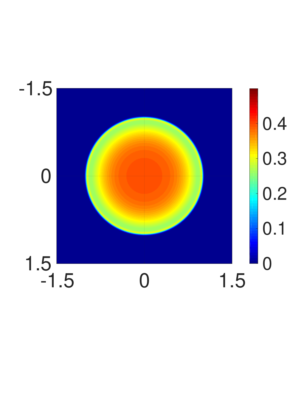
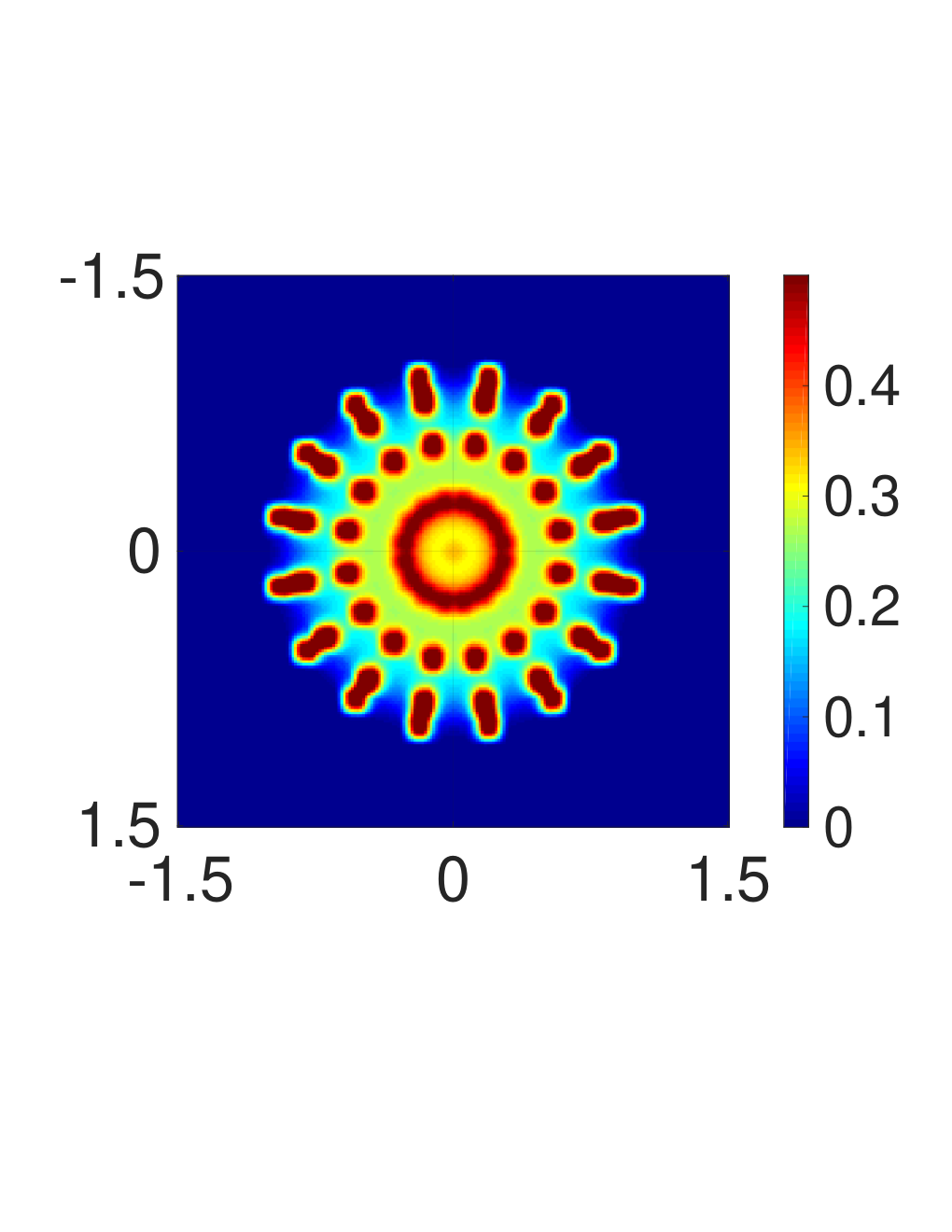
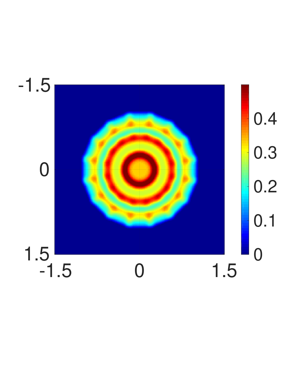
The exact solution has the property of being rotationally symmetric, which is especially violated by the SN method, since the solution suffers from ray effects. By rotating the ordinates of the SN method around the z-axis, one mitigates ray effects. However, oscillations are still present in the radial dimension, because we only rotate around the -axis.
4 Three-dimensional case
To generalize the procedure explained in Section 3 to rotations around an arbitrary axis, we need a quadrature set that allows for easy interpolation of the rotated points in every spatial cell. For this purpose, a quadrature set that is the result of an underlying triangulation of the unit sphere is chosen. Given this triangulation, function values at rotated points can be interpolated via barycentric interpolation on the sphere. The quadrature points and weights, as well as the triangulation, result from projecting a triangulation of planar triangles onto the sphere.
4.1 Quadrature points
For the quadrature points, consider one face of the standard octahedron, i.e. the triangle with nodes and . This triangle is now triangulated in an equidistant way as shown in Fig. 2 on the left. All vertices of the triangulation are projected onto the unit sphere in a next step, presented Fig. 2 on the right.

With being the number of points on the line segment between the points and , and therefore between and , as well as between and , the total number of quadrature points on the whole sphere, denoted by , is given by the relation . Each vertex belongs to six distinct triangles, except for the six vertices at the poles which only belong to four distinct triangles.
Our construction of the quadrature set is very similar to the idea of the TN quadrature [24]. However, instead of taking the midpoints of the resulting triangles in Fig. 2, we take the surrounding vertices. This changes the number of quadrature points that are being generated and the corresponding weights. More importantly however, it directly yields a connectivity between quadrature points which we use for the interpolation later on. For the TN quadrature, it is not clear how to connect vertices from different octants. Our proposed quadrature does not suffer from this ambiguity since vertices fall on the connecting edges between the octants, thus allowing us to keep a triangulation for the whole unit sphere.
4.2 Quadrature weights
For each quadrature point, the quadrature weight corresponds to the area associated with that given point. This area is defined by first connecting the midpoints of all surrounding triangles on the unprojected grid and then projecting this shape onto the surface of the unit ball. For the poles, the resulting shape is a quadrilateral and a hexagon for all other points.
The complete set of quadrature weights is shown in Fig. 3, together with the corresponding hexagons or quadrilaterals. Due to symmetry, it is sufficient to compute the quadrature weights on a single octant and then copy them to all seven other octancts. We observe the smallest quadrature weights for the poles. This is due to two effects. Firstly, the increase of the corresponding area when projecting it onto the unit sphere is smaller than for other points. Secondly, only four neighboring triangles contribute to the quadrature weights at the poles, as opposed to six for all other points.

4.3 Accuracy
We now integrate certain functions on the sphere with the described quadrature to check the implementation and investigate its accuracy. A more detailed analysis of the quadrature rule, and possible improvements, will be the topic of a folllow-up paper. We consider functions, mapping from to and compute the error for different numbers of quadrature points against the analytic solution. The two functions used to test the accuracy of the chosen quadrature are
In Table 4.3 we show the errors resulting from the numerical integration with the quadrature set of the specified order . Integrated were two different functions and . The error ratio is the absolute value of the ratio of two consecutive errors. The results show, that the order of convergence is two with respect to , which implies a first order convergence with respect to the number of quadrature points . First order convergence was expected from the construction. We did not aim for a high order quadrature rule, as we are primarily using the described quadrature due to its low variance in quadrature weights and the naturally arising interpolation capabilities.
| Error for | Error ratio | Error for | Error ratio | ||
|---|---|---|---|---|---|
| 2 | 6 | -0.359039 | - | 2.46015 | - |
| 4 | 38 | -0.012968 | 27.6865 | 0.073617 | 33.4183 |
| 8 | 198 | -0.00234195 | 5.53729 | 0.0265397 | 2.77384 |
| 16 | 902 | -0.000530132 | 4.41767 | 0.00607712 | 4.36715 |
| 32 | 3846 | -0.000125148 | 4.23606 | 0.00143802 | 4.22602 |
| 64 | 15878 | -3.03595e-05 | 4.12219 | 0.000349035 | 4.11999 |
4.4 Rotation and interpolation
Rotation of the quadrature set is straight forward. A rotation is defined by an axis with and a rotation magnitude . For a quadrature point , rotates around by an amount , with the rotation matrix
| (16) |
When performing the rotation of the quadrature points, the associated quadrature weights are kept. The same holds true for the connectivity between the vertices that define the triangulation.
In a next step, we interpolate function values on the rotated quadrature point set, given function values on the original quadrature point set. To do so, we use the triangulation that was set up to create the quadrature points originally. Each rotated point falls into one triangle of the original triangulation. We can then interpolate a function value for any rotated point by the three function values at the vertices belonging to the triangle that the rotated point lies in. Interpolation is then performed via barycentric interpolation. The barycentric interpolation is visualized in Fig. 4 for the planar case. When interpolating a new function value at , we sum the function values at with weights for and being the area of the triangle. For the spherical case, all areas are computed as areas on the unit sphere.
Before computing the relevant interpolation weights, we need to find the corresponding triangle that a quadrature point has been rotated into. As we will restrict ourselves to small rotations later on, these triangles are the neighboring triangles for any quadrature point. However, the interpolation procedure works for any rotation magnitude. Since each spatial cell has the same set of quadrature points, the interpolation weights have to be computed only once. Afterwards, the interpolation can be performed in each spatial cell separately.
4.5 Modified equation for the planar case
We will now consider a simplified setting to explore the effects of the rotation and interpolation step analytically. The fact that the quadrature is still anisotropic makes the analysis on the sphere difficult. We postpone a more detailed discussion to the end of this subsection.
Assume therefore a triangulation in planar geometry with equilateral triangles that is being translated by a vector , where . An excerpt of the original points, together with the surrounding triangles is shown in black and the shifted points with the corresponding triangles in dashed red in Fig. 5. Each point in the original set of points is being shifted to a new point .
The interpolation weights are again the barycentric weights, shown in Fig. 4, that is and , with being the area of the equilateral triangle. The interpolation weights can be computed analytically and expressed in terms of and as
The interpolated function value at is then given by
Similarly we compute expressions for and . If we now reverse the shift by moving all points into the direction , we can interpolate a new value for the point that is
| (17) |
Note that the exact same result would hold in the case of an equilateral triangle with sides of length when the shift is performed by . In order to identify the differential operator that the derived stencil approximates, we perform a Taylor expansion around , where we use the coordinate axis and . These are the axes that run along the hexagonal grid, centered in , show in Fig. 6. From this, we obtain
Plugging this into the derived stencil (17) gives
Instead of writing the derivatives in dependency of and we transform the derivatives to only rely on the direction and the direction perpendicular to , namely .
From the geometry of Fig. 6 follows
Together with
we obtain
Next, we substitute with to obtain
Here, we defined the following constants
which are visualized in Fig. 7.
Finalizing the change of coordinate systems, we derive
| (18) |
We are now going to draw some conclusions from this derivation. First, we observe a diffusive behavior, where diffusion is strongest along the direction of shifting. Furthermore, when the shift is performed in alignment with the lattice, diffusion only occurs along that direction.
Comparing equation (18) with (13) we observe a similar scaling behavior of the diffusion term. Choosing again results in vanishing diffusion for a refinement of the angular discretization (). Since scales like the number of angular quadrature points , we will perform rotations by instead of . This is due to the fact that is not constant for the different triangles on the sphere, it does however scale like .
The implementation of the rSN method differs from this simplified analysis. There, we are moving the quadrature points on the sphere and not in planar geometry. Furthermore, not all triangles have the same size. Additionally, determining the corresponding points from which we interpolate the function values is not trivial. It might happen, that two rotated points fall into the same triangle of the old quadrature set. In the implementation of the rSN method, we also rotate randomly around different axes and perform the usual SN update, i.e. stream and collide, in between interpolating. All these aspects make the theoretical analysis significantly more difficult than for the simplified planar geometry. However, the numerical results indicate a diffusive behavior which is equally strong in any direction. We believe that randomly choosing a rotation axis has an averaging effect. That is, diffusion will be equally strong along all directions since we rotate differently in each time step. As we are no longer restricted to rotations around the z-axis only, diffusion is also not restricted to occur in the azimuthal angle.
A different way to interpret the newly induced diffusion is artificial scattering. Rotating the quadrature set and interpolating the angular flux can be seen as particles scattering into new directions. As it is the case for scattering, the rotation and interpolation procedure is conservative by construction. Furthermore, as described in Alg. 3, we can write the interpolation procedure as . Here, is the angular flux in a given spatial cell before the rotation and interpolation step and is the angular flux at the new quadrature points after the rotation and interpolation step. The matrix contains the interpolation weights and has only three non zero elements per row. It does not depend on the spatial cell index, but is different for each time step since the rotation axis differs from time step to time step. Thus, the angular flux at "scatters" into the directions for which it is used to interpolate function values at the new quadrature set. Since more scattering implies fewer ray-effects, the rSN method mitigates these undesired effects.
5 Implementation
The method can easily be implemented into an existing code for the discrete ordinates method as it is minimally inversive. Only the construction of the quadrature set has to be modified and a function for the rotation and interpolation has to be implemented. In Alg. 1 we see the main components of a discrete ordinates method. We assume available routines that return the quadrature points and quadrature weights given an order , indicated by getOctahedronQuadraturePoints(N) and getOctahedronQuadratureWeights(N). These implementations are in accordance with the explanation in Section 4.1 and Section 4.2. For the standard SN method, the number of quadrature points in the angular variable scales as . Inside the while loop, the angular flux is updated via a finite volume scheme as described in Section 2.3. The modifications that have to be implemented to obtain the rSN method are then highlighted in blue in Alg. 2.
The algorithm that performs the rotation and interpolation in line 11 is presented in Alg. 3. Here we assume that a method to determine the triangle into which a rotated quadrature point falls into is available. Such a method can easily be implemented in an efficient way as we can assume that any point will fall into one of its six neighboring triangles. After having found the corresponding triangle, the interpolation weights are being computed and stored in a matrix as explained in Alg. 3 in line 11 to 14. After having computed the interpolation weights, the interpolation is applied in each spatial cell. We only need to compute the interpolation weights once since the quadrature set is the same in each spatial cell. Alg. 3 is furthermore well suited for parallel implementations.
In general, we cannot expect the interpolation procedure to be conservative. It does however preserve positivity. One way to force the method to be conservative, is by rescaling the scalar flux at each quadrature point, such that the mass before the interpolation step is conserved in each cell separately.
In our comparisons, rSN with is different from traditional SN (relying on a tensorized angular grid as described in Section 3), because we use different quadrature sets. We have included both in the comparisons to distinguish the effect of the new quadrature from the rotation procedure. Furthermore, due to the different relation between and , we will later on compare the methods according to their total number of quadrature points and not their order .
The rotation magnitude is scaled by , shown in line 11 of Alg. 2. This makes the observable effect of the rotation not depend on different time step sizes.
Since the matrix in Alg. 3 contains only three nonzero entries per row, the procedure can also be implemented in a sparse manner. For readability, we chose not to do so in this example.
In all numerical experiments, we observed an increase of the runtime by to when adding the rotation and interpolation procedure to the standard SN implementation. Within the context of all performed simulations we use the implementation of the rSN method as described in Alg. 2. To compare simulations with different rotations strengths we denote by rδSN the rSN method with rotation strength .
5.1 Alternative implementations
Implementing the rotation and interpolation step into the standard SN method is possible in several ways. We will now describe two of these modified implementations. All numerical simulations were performed with the method described above. This is due to the fact that all tested implementations show similar qualitative behavior. This indicates the importance of the presence of the interpolation and rotation step. For example the order in which these steps are being executed as well as other details play a smaller role.
Rotating forth and back
One implementation performed a rotation around a random axis with strength in one time step, followed by a rotation with strength around the same axis in the next time step. This procedure is similar to the idea described in Sec. 4.5 and allowed to perform a more rigorous theoretical analysis, but showed no differences in the computed solution.
Two opposite rotations within one time step
The proposed implementation requires to update the quadrature set outside of the rotation and interpolation step. There might be implementations of the SN method were this is not possible. In those cases, two opposite rotations can be performed within one time update. This keeps the quadrature set outside the rotation and interpolation procedure fixed. To observe the same qualitative behavior as for the proposed rSN implementation, two rotations with and have to be performed instead of one rotation with .
6 Numerical results
In the following, we show results obtained with the standard SN method, as well as with the rSN method. Our results can be reproduced with the freely avaliable code [4]. To demonstrate the properties of ray effect mitigation, we choose test cases that are prone to this behavior.
6.1 The line-source problem
The first problem we look at is the line-source problem. In this test case, the solution is projected onto the -plane, i.e. the spatial domain is . There is only one medium with cross sections . The initial density distribution is a dirac in the center of the spatial domain , , i.e. we have
Numerically, the initial condition is approximated by
| (19) |
with close to zero (see Tab. 2). We vary the number of quadrature points as well as the rotation strength to study effects on the solution. We use a second-order scheme with a minmod slope limiter in space as well as Heun’s method in time. The code used in this work is a re-implementation of [8].
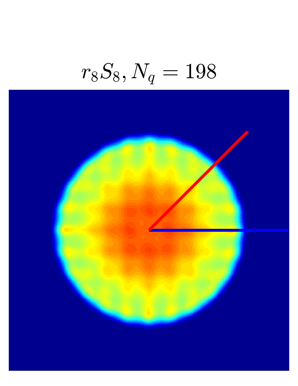
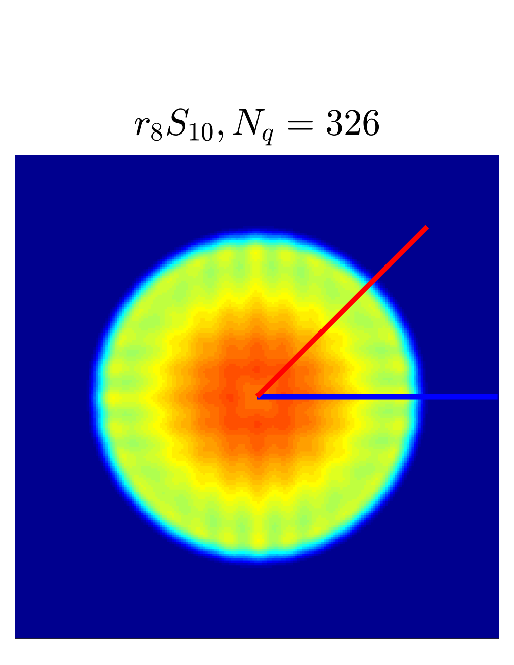
The results of the densities for the line-source problem can be found in Fig. 10. Fixed parameters used in the computation can be found in Table 2.
| , | spatial domain |
|---|---|
| , | number of spatial cells |
| end time | |
| parameters of initial condition (19) | |
| , | cross sections of material |
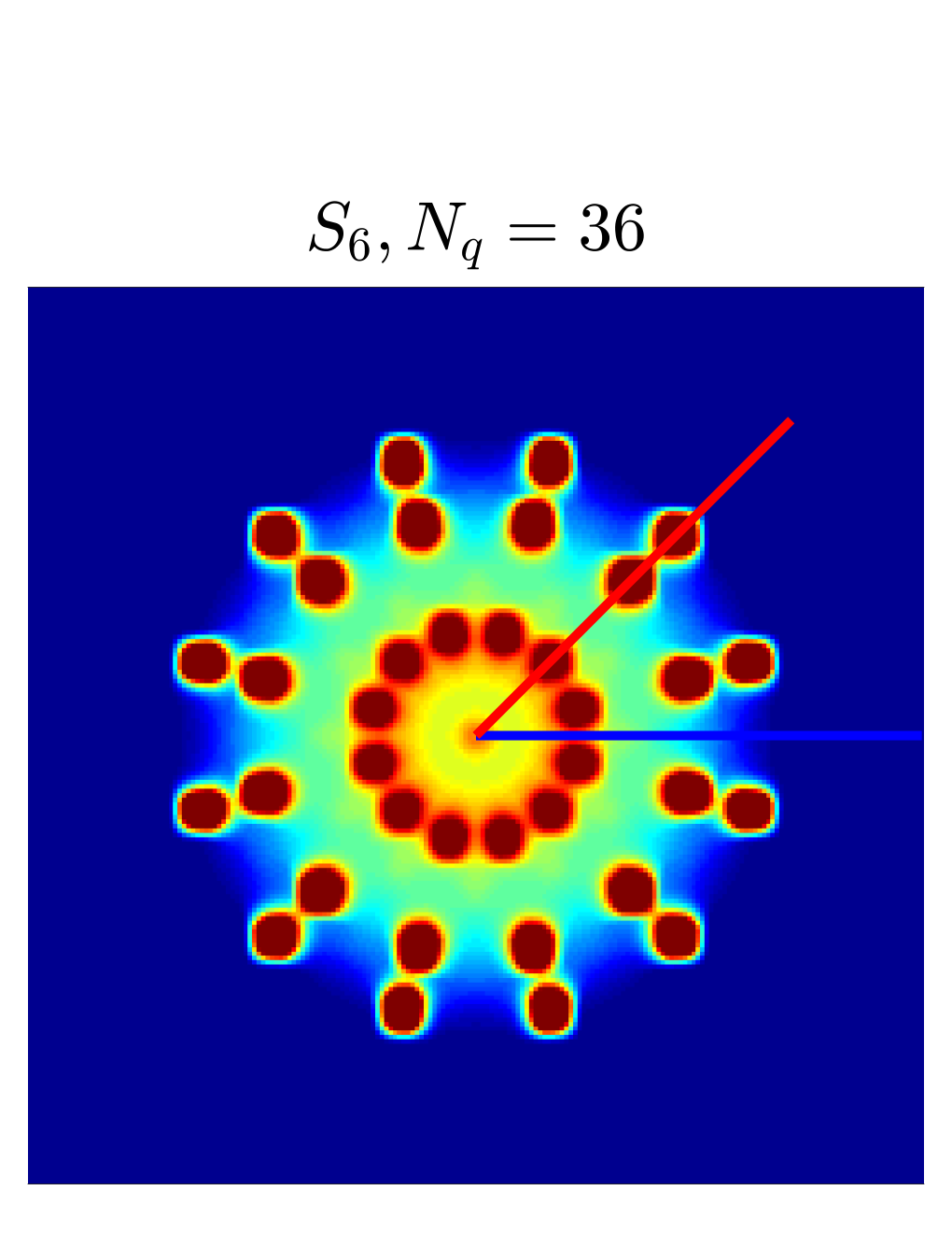
The first row of Fig. 9 shows the density for the line-source problem, computed with the standard SN method for different numbers of quadrature points. Ray effects are predominant especially for the computations with 36 and 64 quadrature points. The solution along the blue horizontal and red diagonal line is shown in Fig. 10 together with the reference solution. While the density along the horizontal cut is mostly underestimated, the solution along the vertical cut is mostly overestimated. Even for 324 quadrature points, the numerical solution has not yet converged against the reference solution.
The second to fourth row show the results for the rSN method with different rotation magnitudes and number of quadrature points, i.e. and . Since the number of quadrature points for the SN method scales different than for the rSN , it is not possible to match the number of quadrature points exactly. For the case of , i.e. no rotation, two quadrature points fall onto another when being projected into the -plane. This effectively halves the number of quadrature points. We still observe ray effects when using the new quadrature set. However, when rotating the quadrature set in every time step by or , the presence of these ray effects reduces dramatically. This can be seen in Fig. 9, but more precisely in Fig 10. The solution along the horizontal and diagonal cut are both closer to another, as well as closer to the reference solution. Oscillations in radial direction can be reduced significantly, which is observable when comparing the first and last row of Fig 10, respectively. When comparing the rSN method for different values of but the same number of quadrature points, we observe a slight decrease in the propagation speed of the solution. The wavefront of the solution slightly moves back for higher values of . However, comparing this with the wavefront of the standard SN method, the rSN method still manages to capture the actual wavefront more accurately in all configurations.
The superiority of the rSN method can be observed when comparing rSN with and against the standard SN method with . With less than a third of the number of quadrature points, the rSN method has fewer oscillations and varies less when comparing the horizontal cut with the diagonal cut. Since the additional computational cost of the rotation and interpolation procedure never exceeds 10%, the rSN method can yield similar, if not better, results for the line-source problem with a third of the costs due to fewer quadrature points. Maybe more importantly, the memory footprint is reduced as well.
6.2 The lattice problem
| , | spatial domain |
|---|---|
| , | number of spatial cells |
| end time | |
| , | cross sections of background |
| , | cross sections of squares |
| strength of isotropic source |

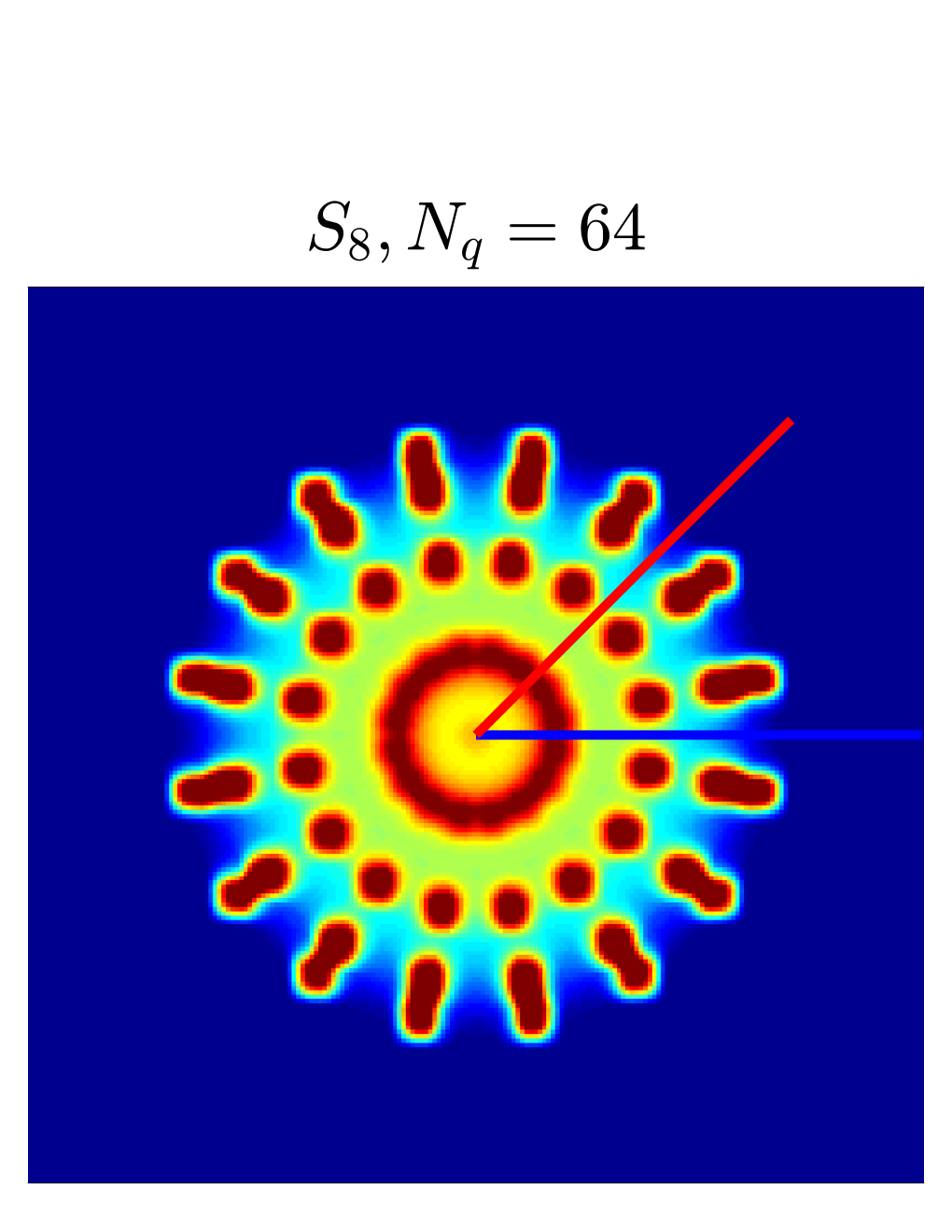
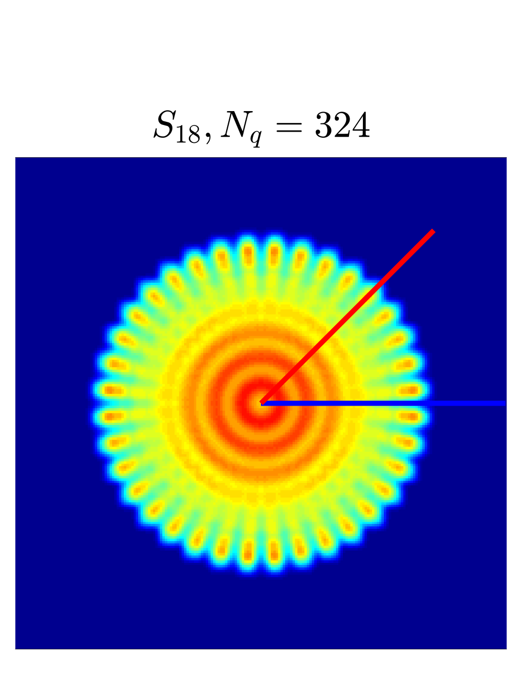
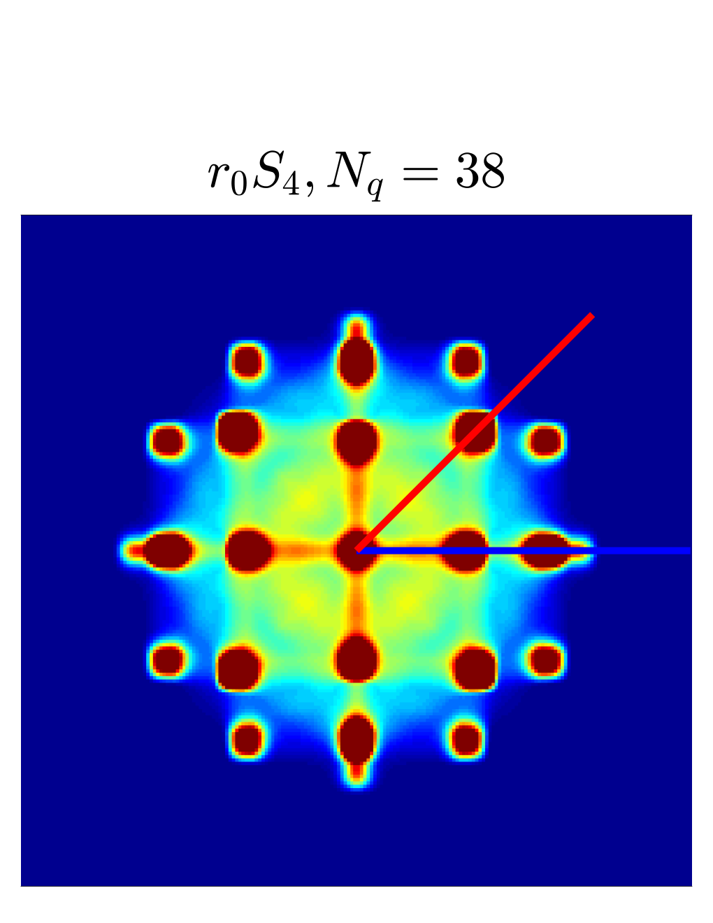
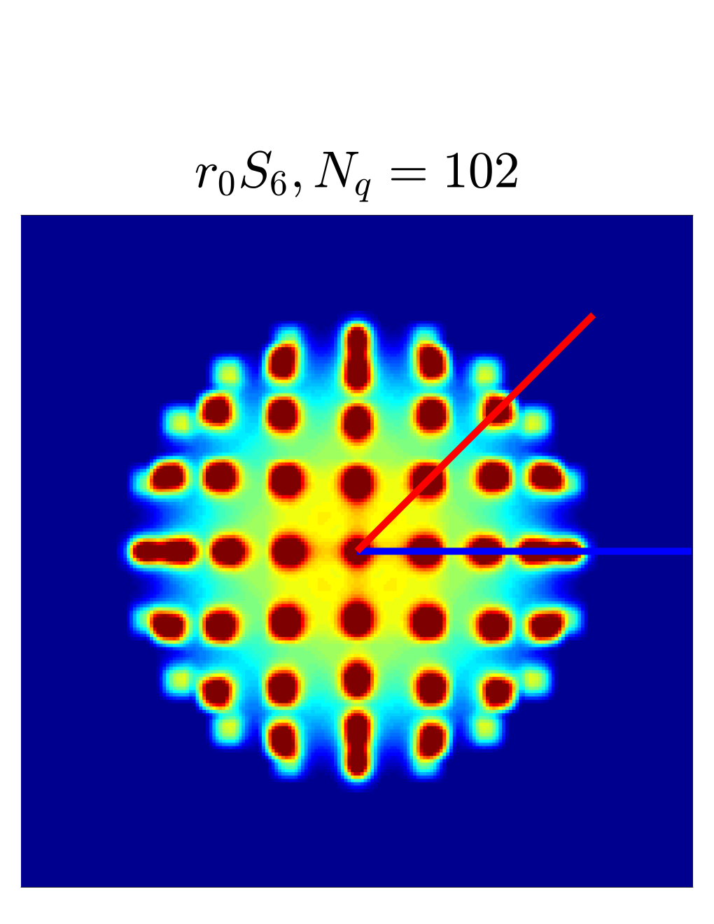
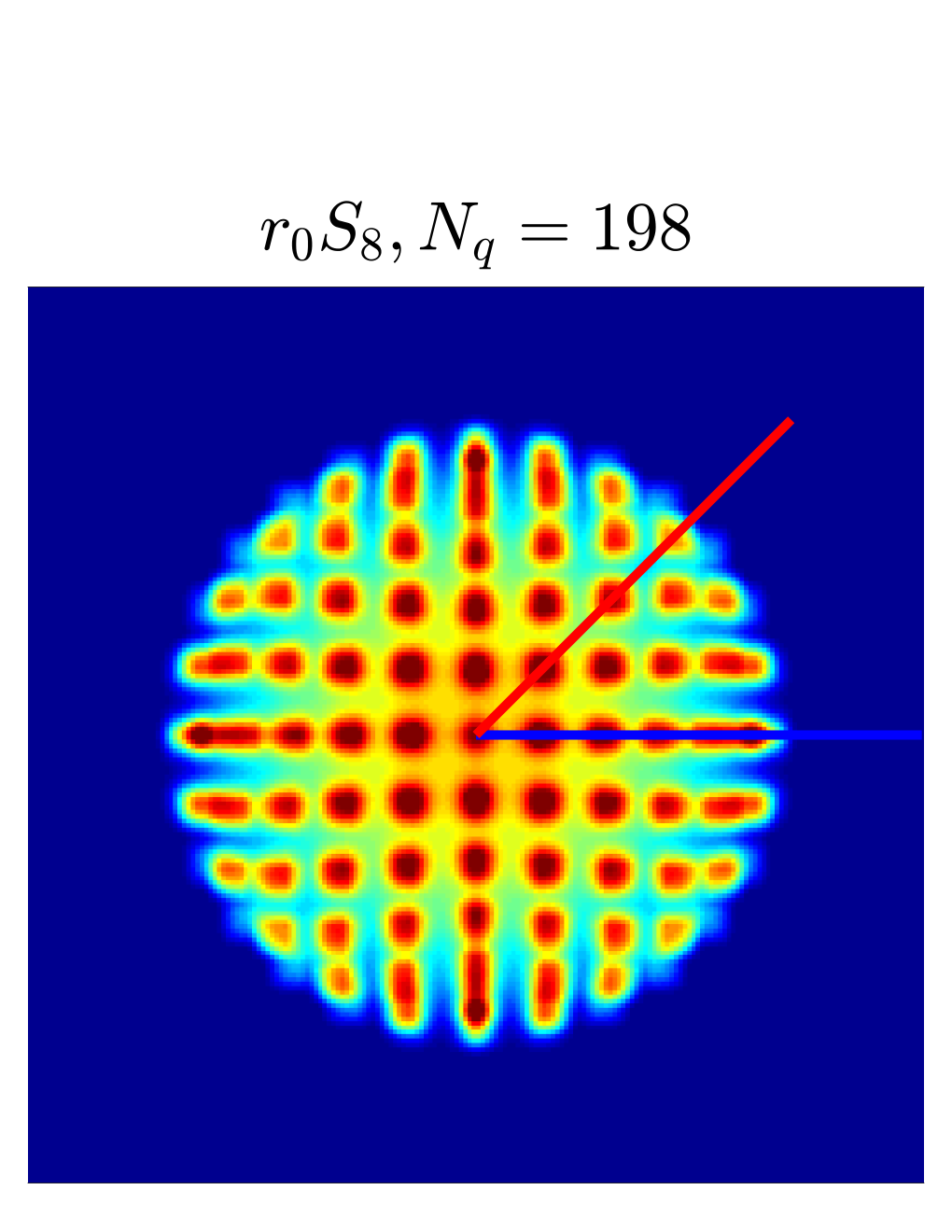
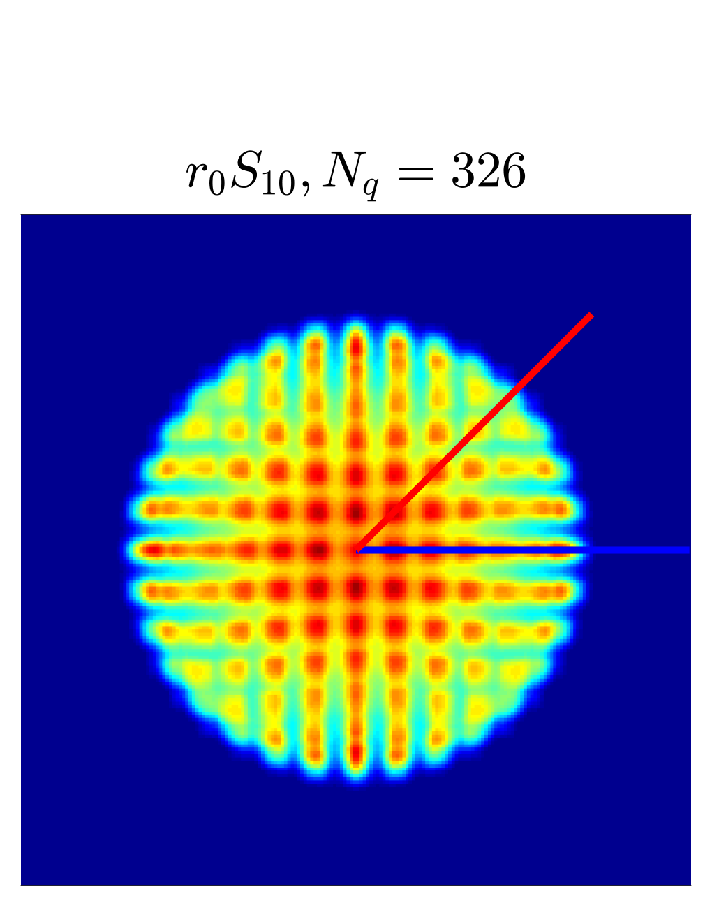
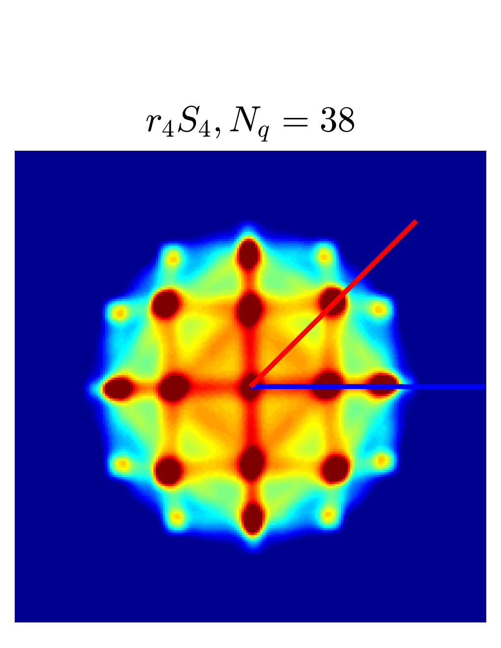
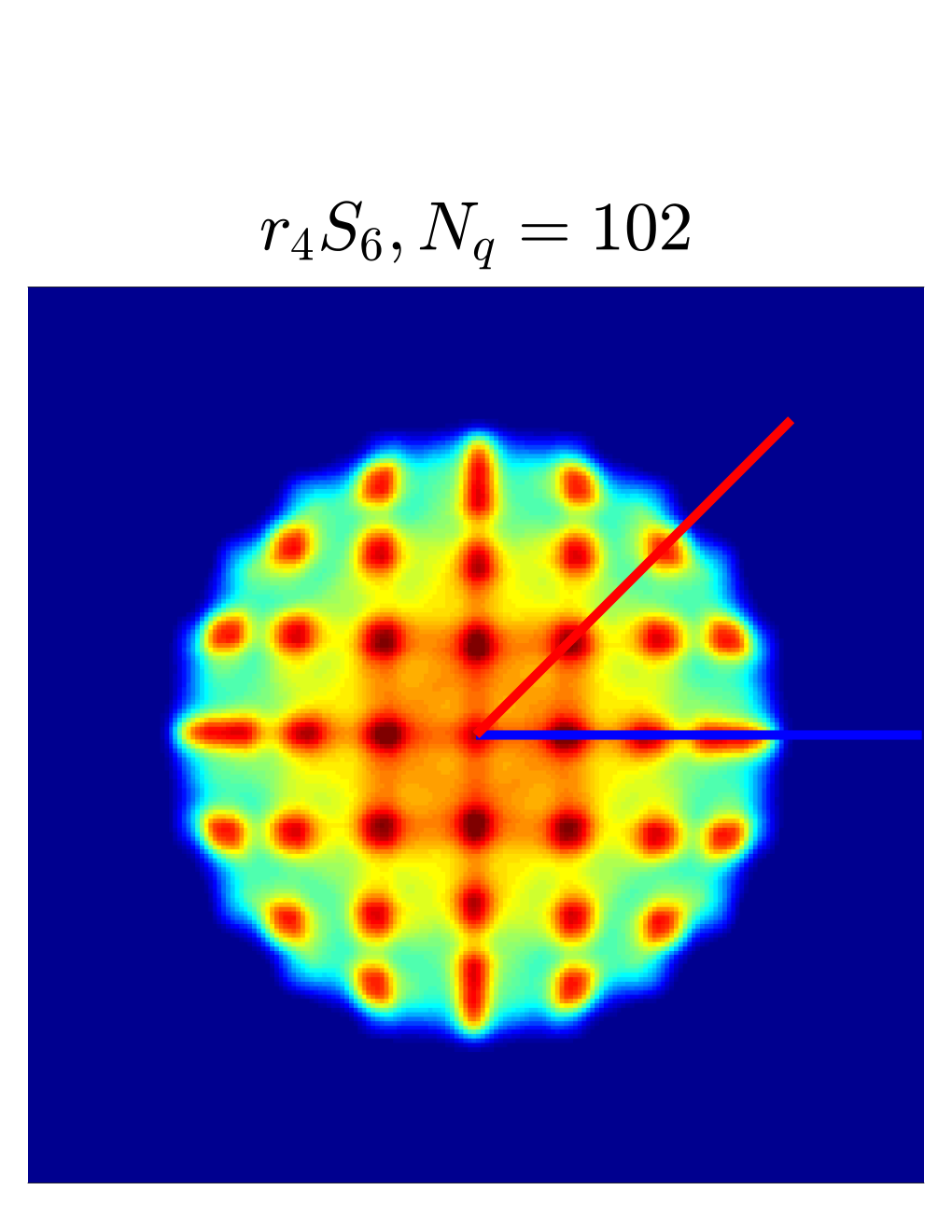
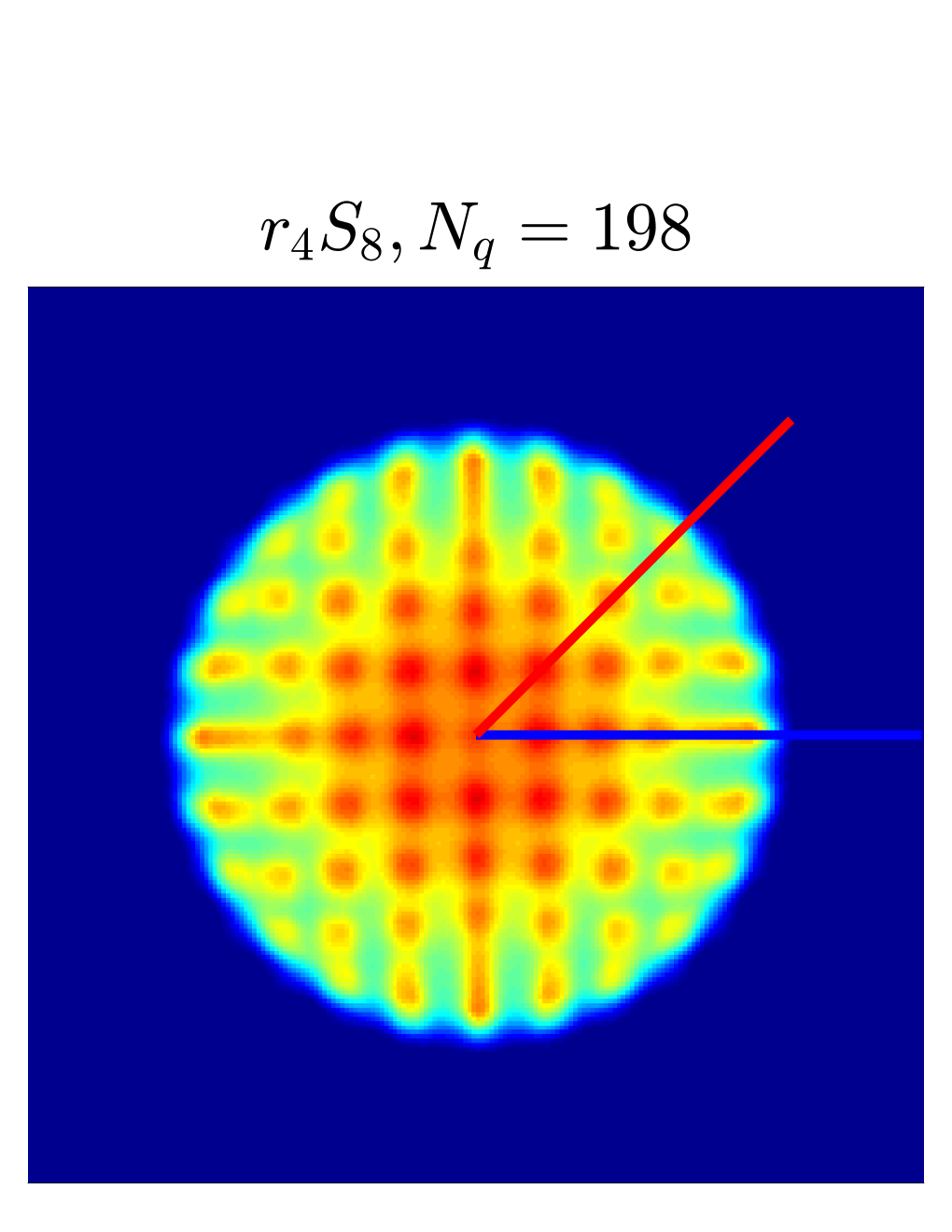
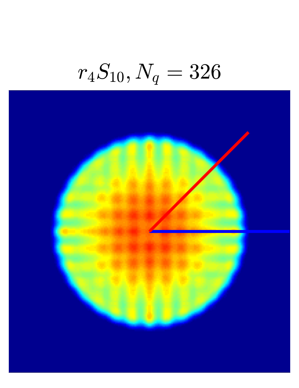
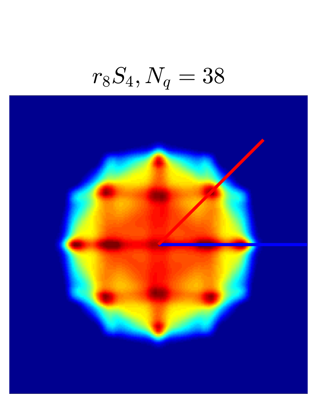
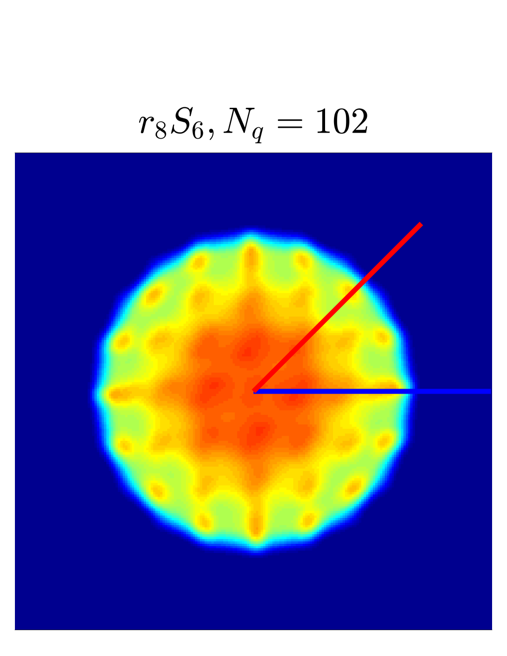
To demonstrate that the rSN method does not only yield satisfactory results for radially symmetric problems, we consider a lattice problem in the second application. The lattice problem simulates a source within a heterogeneous material. The two-dimensional physical space consists of multiple materials, namely a set of squares belonging to a strongly absorbing medium as well as a strongly scattering background [2, 3]. Furthermore, an isotropic source is placed into the center of the physical domain. There is no initial distribution of particles. Particles solely enter the domain by the source term isotropically. Again, we investigate the solution’s dependency on the number of ordinates and the rotation strength. The used parameters, as well as the underlying layout are shown in Tab. 3 and Fig. 8, respectively. The results are summarized in Fig. 11 with the logarithmic density distribution along the horizontal (blue) and vertical (red) cut shown in Fig. 12. Similar to the line-source problem, we organize the plots such that similar number of quadrature points can be found in every column and the rotation strength is fixed within one row. The first row shows the result for the standard SN method, all following rows show the solution of the rSN method with increasing rotation strength. Up to quadrature points we observe ray effects in the SN method, shown in the last column of the first row in Fig. 11. The solution along and still shows oscillatory behavior, seen in Fig. 12. As before, the rSN method without rotation (i.e. ) shows similar ray effects compared to the standard SN method. While these ray effects are similar in structure and strength, the direction of the rays is slightly different due to the different quadrature set. Activating the rotation with or in the third and fourth row visibly diminishes the ray effects. For , the ray effects seem to be diminished with and for with , respectively. Remarkable is the absence of strong ray effects for all number of quadrature points with activated rotation. A convergent behavior of the solution along the horizontal and vertical cut can also be observed in Fig. 12. The last two rows indicate a quality that is not matched by the standard SN method. For the checkerboard case, the rotation strength influences the solution in a less significant way then for the line-source problem.



7 Summary and outlook
To mitigate ray effects of the SN solution, we have introduced a rotation of the quadrature set. By choosing a mesh-based quadrature rule, we enabled an efficient interpolation step to compute the solution values at the rotated quadrature nodes. In addition to mitigating ray effects, the rSN method is easy to implement and promises positivity of solution values. It can be shown analytically that in a simplified setting, the rotation and interpolation step adds a diffusive term of the numerical discretization. Furthermore, we have provided a guideline on how to choose the rotation angle depending on time step and angular grid.
We tested our method on the line-source and lattice problems, and observed a mitigation of ray effects.
Future work will focus on a rigorous analysis of the modified equations when performing a general 3D rotation step. Furthermore, different mesh-based quadrature sets should be studied to identify a quadrature rule with desirable properties, such as homogeneity of integration weights. Additionally, different versions on the rSN method need to be compared. These for example include back and forth rotation before streaming. In an implicit or steady state transport calculation, the ability to perform transport sweeps is of key importance. As the method has been presented, it is not directly compatible with sweeping because the rotation might actually change the face of the boundary from which the solution is propagated. However, one could solve a modified equation directly (without rotations). This will also be investigated in future work.
Acknowledgements
The authors acknowledge many fruitful discussions with Cory D. Hauck (Oak Ridge) and Ryan G. McClarren (Notre Dame).
References
- [1] I. Abu-Shumays, Angular quadratures for improved transport computations, Transport Theory and Statistical Physics, 30 (2001), pp. 169–204.
- [2] T. A. Brunner, Forms of approximate radiation transport, Sandia report, (2002).
- [3] T. A. Brunner and J. P. Holloway, Two-dimensional time dependent Riemann solvers for neutron transport, Journal of Computational Physics, 210 (2005), pp. 386–399.
- [4] T. Camminady, M. Frank, K. Kuepper, and J. Kusch, Source code rSn method, 2018, https://git.scc.kit.edu/qd4314/rSN.
- [5] K. M. Case and P. F. Zweifel, Linear transport theory, (1967).
- [6] J. Fleck Jr and J. Cummings Jr, An implicit Monte Carlo scheme for calculating time and frequency dependent nonlinear radiation transport, Journal of Computational Physics, 8 (1971), pp. 313–342.
- [7] C. L. Fryer, G. Rockefeller, and M. S. Warren, SNSPH: a parallel three-dimensional smoothed particle radiation hydrodynamics code, The Astrophysical Journal, 643 (2006), p. 292.
- [8] C. K. Garrett and C. D. Hauck, A comparison of moment closures for linear kinetic transport equations: The line source benchmark, Transport Theory and Statistical Physics, 42 (2013), pp. 203–235.
- [9] J. Jung, H. Chijiwa, K. Kobayashi, and H. Nishihara, Discrete ordinate neutron transport equation equivalent to PL approximation, Nuclear Science and Engineering, 49 (1972), pp. 1–9.
- [10] K. Lathrop, Remedies for ray effects, Nuclear Science and Engineering, 45 (1971), pp. 255–268.
- [11] K. D. Lathrop, Ray effects in discrete ordinates equations, Nuclear Science and Engineering, 32 (1968), pp. 357–369.
- [12] R. J. LeVeque, Numerical Methods for Conservation Laws. 1992, BirkhaØ user Basel.
- [13] E. E. Lewis and W. F. Miller, Computational methods of neutron transport, (1984).
- [14] M. Marinak, G. Kerbel, N. Gentile, O. Jones, D. Munro, S. Pollaine, T. Dittrich, and S. Haan, Three-dimensional HYDRA simulations of National Ignition Facility targets, Physics of Plasmas, 8 (2001), pp. 2275–2280.
- [15] K. A. Mathews, On the propagation of rays in discrete ordinates, Nuclear science and engineering, 132 (1999), pp. 155–180.
- [16] M. K. Matzen, M. Sweeney, R. Adams, J. Asay, J. Bailey, G. Bennett, D. Bliss, D. Bloomquist, T. Brunner, R. e. Campbell, et al., Pulsed-power-driven high energy density physics and inertial confinement fusion research, Physics of Plasmas, 12 (2005), p. 055503.
- [17] R. G. McClarren and C. D. Hauck, Robust and accurate filtered spherical harmonics expansions for radiative transfer, Journal of Computational Physics, 229 (2010), pp. 5597–5614.
- [18] W. Miller Jr and W. H. Reed, Ray-effect mitigation methods for two-dimensional neutron transport theory, Nuclear Science and Engineering, 62 (1977), pp. 391–411.
- [19] J. Morel, T. Wareing, R. Lowrie, and D. Parsons, Analysis of ray-effect mitigation techniques, Nuclear science and engineering, 144 (2003), pp. 1–22.
- [20] G. C. Pomraning, The equations of radiation hydrodynamics, Courier Corporation, (1973).
- [21] W. H. Reed, Spherical harmonic solutions of the neutron transport equation from discrete ordinate codes, Nuclear Science and Engineering, 49 (1972), pp. 10–19.
- [22] F. D. Swesty and E. S. Myra, A numerical algorithm for modeling multigroup neutrino-radiation hydrodynamics in two spatial dimensions, The Astrophysical Journal Supplement Series, 181 (2009), p. 1.
- [23] J. Tencer, Ray effect mitigation through reference frame rotation, Journal of Heat Transfer, 138 (2016), p. 112701.
- [24] C. Thurgood, A. Pollard, and H. Becker, The TN quadrature set for the discrete ordinates method, Journal of heat transfer, 117 (1995), pp. 1068–1070.