Compressive Sensing for cut improvement and local clustering.

Ming-Jun Lai Note: mjlai@uga.edu. Department of Mathematics, University of Georgia, Athens, GA 30602. This research is partially supported by the National Science Foundation under the grant #DMS 1521537. Daniel Mckenzie Note: mckenzie@math.ucla.edu. Department of Mathematics, University of California, Los Angeles, CA 155505. The financial assistance of the National Research Foundation of South Africa (NRF) towards this research is hereby acknowledged. Opinions expressed and conclusions arrived at, are those of the author and not necessarily to be attributed to the NRF. This research was conducted while this author was a graduate student at the University of Georgia and he gratefully acknowledges support and encouragement received from the Math Department of UGA.

August 24, 2026

Abstract

We show how one can phrase the cut improvement problem for graphs as a sparse recovery problem, whence one can use algorithms originally developed for use in compressive sensing (such as SubspacePursuit or CoSaMP) to solve it. We show that this approach to cut improvement is fast, both in theory and practice and moreover enjoys statistical guarantees of success when applied to graphs drawn from probabilistic models such as the Stochastic Block Model. Using this new cut improvement approach, which we call ClusterPursuit, as an algorithmic primitive we then propose new methods for local clustering and semi-supervised clustering, which enjoy similar guarantees of success and speed. Finally, we verify the promise of our approach with extensive numerical benchmarking.

Keywords: Cluster Extraction, Local Clustering, Cut Improvement, Semi-Supervised Clustering, Community Detection, Compressive Sensing, Sparse Solution, Graph Laplacian.

1 Introduction

Finding clusters is a problem of primary interest when analyzing graphs. This is because vertices which are in the same cluster can reasonably be assumed to have some latent similarity. Thus, clustering can be used to find communities in social networks [24, 48, 53] or deduce political affiliation from a network of blogs [5]. Moreover, even data sets which are not presented as graphs can profitably be studied by first creating an auxiliary graph (eg. a $K$ - or $\epsilon$ -nearest-neighbors graph) and then applying graph clustering techniques. This has been successfully applied to image segmentation [43, 37], image classification [30] and natural language processing [19].

Refer to caption — Figure 1: Left: the College Football graph of [24]. Vertices represents colleges fielding (American) football teams in the 2000 season. Vertices are connected if the respective teams played each other during the regular season. Clusters correspond to the various conferences in which teams play. Note that there are five schools, denoted in black, which are “independents” ie they are not affiliated with any conference. These can be thought of as background vertices. Middle: Senate co-voting for the 97th Congress, created using data from [32]. Vertices represent Senators and are connected if the respective Senators cast the same vote on a majority of bills. The two large clusters correspond to the two major American political parties. Notice how the blue cluster can be visually subdivided into two sub-clusters. Right: The OptDigits dataset consists of $5620$ grayscale images of handwritten digits 0–9 of size $8\times 8$ . We discuss how to turn this into a graph in §10. Note that as there are ten digits, we expect this graph to have ten disjoint clusters.

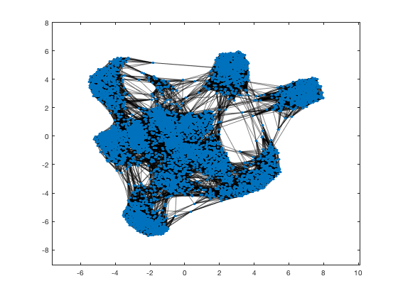
We shall informally think of a cluster as a subset of vertices, $C\subset V$ with many edges between vertices in $C$ , and few edges to the rest of the graph, $C^{c}$ . See Figure 1 for a few examples. While some graphs may allow a neat partitioning into disjoint clusters (for example the OptDigits graph in Figure 1), for many graphs this is not the case. Some graphs may contain background vertices, that is, vertices which do not belong to any cluster (see the College Football graph in Figure 1). Alternatively, graphs may exhibit clusters at multiple scales (See the Senate Co-voting graph in Figure 1). In many cases, one has certain a priori information that could be used to improve clustering. For example in the OptDigits graph, we may know that some small subset, $\Gamma\subset V$ , all represent images of ones. It is reasonable to assume that algorithms which incorporate this additional information (usually referred to as semi-supervised algorithms) will perform better than ones which do not. With this in mind, it is convenient to appeal to the following taxonomy of clustering algorithms:

1.

Global clustering algorithms assign every vertex to one of $k$ clusters, where the clusters may or may not be disjoint. Algorithms for this problem may be unsupervised (for example SpectralClustering [43, 40] or GenLouvain [18]) or semisupervised (for example the auction dynamics approach of [30], or the regional force based methods of [54]). This is appropriate for graphs such as the OptDigits graph of Figure 1, where one expects a clear partition of the vertices into clusters.
2.

Local clustering algorithms¹¹ 1 Also known as cluster extraction algorithms in the statistics literature take as input a small set of “seed vertices”, $\Gamma\subset V$ and return a good cluster containing $\Gamma$ . Algorithms for local clustering are not confounded by background vertices, as they are not required to assign them to a cluster. One can further sub-divide local clustering algorithms into strongly and weakly local clustering algorithms. Strongly local algorithms, for Nibble [45, 46], PPR-Grow [1] or CapacityReleasingDiffusion [52], are characterized by having run time proportional to the size of the cluster found. This is advantageous when the cluster in question has much fewer vertices than the graph as a whole. Weakly local algorithms are characterized as having run time proportional to the size of $G$ . In practice they are frequently faster than strongly local algorithms when finding large or moderately large clusters. We note that both kinds of local clustering algorithms may take as input a scale parameter, which dictates the size of the output cluster returned. This is useful when the graph at hand contains clusters at multiple scales, such as the Senate co-voting graph of Figure 1.
3.

Cut improvement algorithms(cf. [1], [41], [50]) take as input a cut, or subset $\Omega\subset V$ , which one can think of as an approximation to a cluster $C$ , and refine it to produce a better approximation. Often cut improvement algorithms are run on the output of a local clustering algorithm to improve the quality of the output.

The central contribution of this paper is a new cut improvement algorithm which we call ClusterPursuit, that phrases the cut improvement problem as a sparse recovery problem. We pair this with a simple local clustering algorithm which we call Random Walk Thresholding or RWThresh to obtain a two-stage weakly local clustering algorithm that we shall refer to as CP+RWT. One can iterate this algorithm to find all clusters in a graph; we call this procedure iterated CP+RWT or ICP+RWT. After presenting some mathematical preliminaries and outlining the assumptions we place on generative models of graphs in §2, we derive the ClusterPursuit algorithm in §3 and prove that, given a cut $\Omega$ satisfying $|C_{1}\bigtriangleup\Omega|/|C_{1}|=O(1)$ ClusterPursuit returns $C_{1}^{\#}$ satisfying $|C_{1}\bigtriangleup C_{1}^{\#}|/|C_{1}|=o(1)$ . Here, $C_{1}$ denotes the smallest cluster in the graph. In §4 we discuss the RWThresh algorithm, and show that given a small set of seed vertices, $\Gamma\subset C_{1}$ , it is capable of finding an $\Omega$ satisfying $|C_{1}\bigtriangleup\Omega|/|C_{1}|=O(1)$ . This leads naturally to guarantees of success for the two-stage local clustering algorithm CP+RWT, which we present in §5. In §6 we briefly discuss ICP+RWT while in §7 we show that CP+RWT and ICP+RWT enjoy a computational complexity of $O(nd_{\max}\log(n))$ where $d_{\max}$ is the largest vertex degree in the graph. In §8 we survey the literature and compare our work with relevant recent work in the area, while in §9 we show that a popular generative model of graphs with communities, namely the stochastic block model, satisfies the assumptions outlined in §2. Finally, we complement theoretical insight with experimental results in §10. In the interest of reproducibility, we make our code available at: danielmckenzie.github.io.

2 Preliminaries

2.1 Graph Notation and Definitions

We restrict our attention to finite, simple, undirected graphs $G=(V,E)$ , possibly with non-negative edge weights. We identify the vertex set $V$ with the integers $[n]:=\{1,\ldots,n\}$ and denote an edge between vertices $i$ and $j$ as $\{i,j\}\in E$ . The (possibly weighted) adjacency matrix of $G$ will be denoted as $A$ . By $d_{i}$ we mean the degree of the $i$ -th vertex, computed as $d_{i}=\sum_{j}A_{ij}$ . For any $S\subset V$ define $\text{vol}(S)=\sum_{i\in S}d_{i}$ . For quantities such as $d_{i}$ (and later $\lambda_{i}$ ) that are indexed by $i\in[n]$ , let $d_{\max}:=\max_{i}d_{i}$ and similarly $d_{\min}:=\min_{i}d_{i}$ . Denote by $D$ the diagonal matrix whose $(i,i)$ entry is $d_{i}$ . By “cluster” we shall mean a subset of vertices, $C\subset V$ , that is well-connected but sparsely connected to the rest of the graph. If a graph has clusters we shall refer to them as $C_{1},\ldots,C_{k}$ . We define $n_{a}:=|C_{a}|$ and assume that the clusters are ordered by size, so that $n_{1}\leq n_{2}\leq\ldots,\leq n_{k}$ . We reserve the letters $a$ and $b$ for indexing clusters, while $i$ and $j$ will index vertices.

Definition 2.1 (Laplacians of graphs).

The normalized, random walk Laplacian is defined as $L=I-D^{-1}A$ . We shall simply refer to it as the Laplacian. The normalized, symmetric Laplacian is: $L^{\text{sym}}:=I-D^{-1/2}AD^{-1/2}$ .

Recall the following elementary result in spectral graph theory (see [49], for example, for a proof):

Theorem 2.2.

Let $C_{1},\ldots,C_{k}$ denote the connected components of a graph $G$ . Then the cluster indicator vectors $\mathbf{1}_{C_{1}},\ldots,\mathbf{1}_{C_{k}}$ form a basis for the kernel of $L$ .

Suppose that $G$ has clusters $C_{1},\ldots,C_{k}$ . By definition, clusters have few edges between them, and so it is useful to write $G$ as the union of two edge-disjoint subgraphs, defined as follows: let $G^{\text{in}}=(V,E^{\text{in}})$ have only edges between vertices in the same cluster, while $G^{\text{out}}=(V,E^{\text{out}})$ consist only of edges between vertices in different clusters. We emphasize that this is a theoretical construction, as in practice we of course cannot ascertain whether two vertices are in the same cluster without first solving the clustering problem, which is precisely what we are trying to do. Denote by $A^{\text{in}}$ and $L^{\text{in}}$ (resp. $A^{\text{out}}$ and $L^{\text{out}}$ ) the adjacency matrix and Laplacian of $G^{\text{in}}$ (resp. $G^{\text{out}}$ ). Similarly, $d_{i}^{\text{in}}$ (resp. $d^{\text{out}}_{i}$ ) shall denote the degree of the vertex $i$ in the graph $G^{\text{in}}$ (resp. $G^{\text{out}}$ ). For future reference we define the random walk transition matrices $P=AD^{-1}$ and $N:=D^{-1/2}AD^{-1/2}$ . We note that the spectra of $P,N,A,L$ are related:

Lemma 2.3.

For any matrix $B$ with real eigenvalues let $\lambda_{i}(B)$ denote the $i$ -th smallest eigenvalue, counted with multiplicity. Then $\lambda_{i}(L)=\lambda_{i}(L^{\text{sym}})$ while $\lambda_{n-i}(N)=\lambda_{n-i}(P)=1-\lambda_{i}(L)$

Proof.

Observe that $L=D^{-1/2}L^{\text{sym}}D^{1/2}$ , hence $L$ and $L^{\text{sym}}$ have the same spectrum. Similarly $P=D^{1/2}\left(I-L^{\text{sym}}\right)D^{-1/2}$ hence $P$ and $N=I-L^{\text{sym}}$ have the same spectrum. Thus if $\lambda$ is the $i$ -th smallest eigenvalue of $L^{\text{sym}}$ it is the $i$ -th largest (and hence the $(n-i)$ -th smallest) eigenvalue of $I-L^{\text{sym}}$ . ∎

For any $S\subset V$ , we denote by $G_{S}$ the induced sub-graph with vertices $S$ and edges all $\{i,j\}\in E$ with $i,j\in S$ . By $A_{G_{S}}$ (resp. $L_{G_{S}}$ ) we mean the adjacency matrix (resp. Laplacian) of the graph $G_{S}$ . Note that $L_{G_{S}}$ is not a submatrix of $L$ ! For any $S\subset[n]$ we define an indicator vector $\mathbf{1}_{S}\in\mathbb{R}^{n}$ by $(\mathbf{1}_{S})_{i}=1$ if $i\in S$ and $(\mathbf{1}_{S})_{i}=0$ otherwise. $|S|$ will always denote the cardinality of $S$ . For any matrix $B$ , by $B_{S}$ we mean the submatrix of $B$ consisting of the columns $b_{i}$ for all $i\in S$ .

2.2 Compressive Sensing

Recall for any ${\bf x}\in\mathbb{R}^{n}$ , $\|{\bf x}\|_{0}:=|\text{supp}({\bf x})|=|\{i:\ x_{i}\neq 0\}|$ is the sparsity of ${\bf x}$ . If $\|{\bf x}\|_{0}\ll n$ we say that ${\bf x}$ is sparse. Candés, Donoho and their collaborators in [20, 9] pioneered the study of compressive sensing, which offers theoretical analysis and algorithmic tools for finding sparse solutions to linear systems $\Phi{\bf x}={\bf b}$ , for example by solving the minimization problem:

\text{argmin}\|\Phi{\bf x}-{\bf y}\|_{2}\text{ subject to }\|{\bf x}\|_{0}\leq s,

(1)

where $\Phi\in\mathbb{R}^{m\times n}$ is referred to as the sensing matrix. Typically, it is assumed that $m\leq n$ although this will not be the case in this paper. There are many algorithms available to solve Problem (1), but the one we shall focus on is the SubspacePursuit algorithm introduced in [17].

Algorithm 1 SubspacePursuit, as presented in [17]

Input variables: measurement matrix $\Phi$ , measurement vector ${\bf y}$ , sparsity parameter $s$ and number of iterations $J$ .

Initialization:

(1)

S^{(0)}=\mathcal{L}_{s}(\Phi^{\top}{\bf y})

(2)

{\bf x}^{(0)}=\argmin_{{\bf z}\in\mathbb{R}^{N}}\{\|{\bf y}-\Phi{\bf z}\|_{2}:\ \supp({\bf z})\subset S^{(0)}\}

(3)

{\bf r}^{(0)}={\bf y}-\Phi{\bf x}^{(0)}

for

j=1:J

(1)

\hat{S}^{(j)}=S^{(j-1)}\cup\mathcal{L}_{s}\left(\Phi^{\top}{\bf r}^{(j-1)}\right)

(2)

\displaystyle{\bf u}=\argmin_{{\bf z}\in\mathbb{R}^{N}}\{\|{\bf y}-\Phi{\bf z}\|_{2}:\ \supp({\bf z})\subset\hat{S}^{(j)}\}

(3)

S^{(j)}=\mathcal{L}_{s}({\bf u})

and

{\bf x}^{(j)}=\mathcal{H}_{s}({\bf u})

(4)

{\bf r}^{(j)}={\bf y}-\Phi{\bf x}^{(j)}

end for

Here $\mathcal{L}_{s}(\cdot)$ and $\mathcal{H}_{s}(\cdot)$ are thresholding operators:

		$\displaystyle\mathcal{L}_{s}({\bf v}):=\{i\in[n]:\ v_{i}\text{ among }s\text{ largest-in-magnitude entries in }{\bf v}\}$
		$\displaystyle\mathcal{H}_{s}({\bf v})_{i}:=\left\{\begin{array}[]{cc}v_{i}&\text{ if }i\in\mathcal{L}_{s}({\bf v})\\ 0&\text{ otherwise. }\end{array}\right.$

In quantifying whether (1) has a unique solution, the following constant is often used (see [21])

Definition 2.4.

The $s$ Restricted Isometry Constant ( $s$ -RIC) of $\Phi\in\mathbb{R}^{m\times n}$ , written $\delta_{s}(\Phi)$ , is defined to be the smallest value of $\delta>0$ such that, for all ${\bf x}\in\mathbb{R}^{n}$ with $\|{\bf x}\|_{0}\leq s$ , we have:

(1-\delta)\|{\bf x}\|_{2}^{2}\leq\|\Phi{\bf x}\|_{2}^{2}\leq(1+\delta)\|{\bf x}\|_{2}^{2}.

If $\delta_{s}(\Phi)<1$ we often say that $\Phi$ has the Restricted Isometry Property (RIP).

One of the reasons for the remarkable usefulness of compressive sensing is its robustness to error, both additive (i.e. in ${\bf y}$ ) and multiplicative (i.e. in $\Phi$ ). More precisely, suppose that a signal $\hat{{\bf y}}=\hat{\Phi}{\bf x}^{*}$ is acquired, but that we do not know the sensing matrix $\hat{\Phi}$ exactly. Instead, we have access only to $\Phi=\hat{\Phi}+M$ , for some small perturbation $M$ . Suppose further that there is some noise in the measurement process, so that the signal we actually receive is ${\bf y}=\hat{{\bf y}}+{\bf e}$ . Can one hope to approximate a sparse vector ${\bf x}^{*}$ from ${\bf y}$ , given only $\Phi$ ? This question is answered in the affirmative way by several authors, starting with the work of [29]. For SubspacePursuit, we have the following result (cf. [33]):

Theorem 2.5.

Let ${\bf x}^{*}$ , ${\bf y}$ $\hat{{\bf y}}$ , $\Phi$ and $\hat{\Phi}$ be as above and suppose that $\|{\bf x}^{*}\|_{0}\leq s$ . For any $t\in[n]$ , let $\delta_{t}:=\delta_{t}(\Phi)$ . Define the following constants:

\epsilon_{{\bf y}}:=\|{\bf e}\|_{2}/\|\hat{{\bf y}}\|_{2}\text{ and }\epsilon^{s}_{\Phi}=\|M\|_{2}^{(s)}/\|\hat{\Phi}\|_{2}^{(s)}

where for any matrix $B$ , $\|B\|_{2}^{(s)}:=\max\{\|B_{S}\|_{2}:\ S\subset[n]\text{ and }|S|=s\}$ . Define further:

\rho=\frac{\sqrt{2\delta_{3s}^{2}(1+\delta_{3s}^{2})}}{1-\delta_{3s}^{2}}\quad\text{ and }\quad\tau=\frac{(\sqrt{2}+2)\delta_{3s}}{\sqrt{1-\delta_{3s}^{2}}}(1-\delta_{3s})(1-\rho)+\frac{2\sqrt{2}+1}{(1-\delta_{3s})(1-\rho)}

Assume $\delta_{3s}\leq 0.4859$ and let ${\bf x}^{(m)}$ be the output of SubspacePursuit applied to Problem (1) after $m$ iterations. Then:

\frac{\|{\bf x}^{*}-{\bf x}^{(m)}\|_{2}}{\|{\bf x}^{*}\|_{2}}\leq\rho^{m}+\tau\frac{\sqrt{1+\delta_{s}}}{1-\epsilon^{s}_{\Phi}}(\epsilon^{s}_{\Phi}+\epsilon_{{\bf y}}).

Proof.

This is Corollary 1 in [33]. Note that our convention on hats is different to theirs — our $\Phi$ is their $\hat{\Phi}$ , hence our $\rho$ is their $\hat{\rho}$ and so on. ∎

Next it is easy to obtain bounds on the quantity $\|B\|_{2}^{(s)}:=\max_{S\subset[n]\atop|S|=s}\|B_{S}\|_{2}$ :

Lemma 2.6.

For any matrix $B$ and any $2\leq s\leq n$ we have that $\sigma_{s-1}(B)\leq\|B\|_{2}^{(s)}\leq\sigma_{\max}(B)=\|B\|_{2}$ , where $\sigma_{j}(B)$ denotes the $j$ -th smallest singular value of $B$ .

Proof.

Observe that, for any matrix $B$ ,

\|B\|_{2}^{(s)}=\max_{S\subset[n]\atop|S|=s}\|B_{S}\|_{2}=\max_{S\subset[n]\atop|S|=s}\sigma_{\max}(B_{S}),

where $\sigma_{\max}(B_{S})$ denotes the maximum singular value of $B_{S}$ . Because $\sigma_{\max}(B_{S})=\sigma_{s}(B_{S})$ , by the interlacing theorem for singular values (cf. [47]) $\sigma_{s-1}(B)\leq\sigma_{\max}(B_{S})\leq\sigma_{\max}(B)$ . ∎

2.3 The Data Model

For conceptual clarity, we shall take an asymptotic viewpoint, and consider graphs $G\in\mathcal{G}_{n}$ as $n\to\infty$ . Note that the graphs under consideration may be weighted or unweighted. We say that a graph property $P$ holds almost surely for $\mathcal{G}_{n}$ if the probability of a $G$ drawn from $\mathcal{G}_{n}$ not having $P$ is $o(1)$ .

Assumptions.

Suppose that there exist $\epsilon_{i}=o(1)$ as $n\to\infty$ for $i=1,2,3$ such that for all $G\in\mathcal{G}_{n}$ :

(A1)

$V=C_{1}\cup\ldots\cup C_{k}$ where the $C_{a}$ are disjoint, planted clusters and $k$ is $O(1)$ as $n\to\infty$ .
(A2)

For all $a\in[k]$ we have that $\lambda_{2}(L_{G_{C_{a}}})\geq 1-\epsilon_{1}$ and $\lambda_{n_{a}}(L_{G_{C_{a}}})\leq 1+\epsilon_{1}$ almost surely.
(A3)

letting $r_{i}:=d^{\text{out}}_{i}/d^{\text{in}}_{i}$ , $r_{i}\leq\epsilon_{2}$ for all $i\in[n]$ almost surely.
(A4)

If $d^{\text{in}}_{\text{av}}:=\mathbb{E}[d^{\text{in}}_{i}]$ then $d^{\text{in}}_{\max}\leq(1+\epsilon_{3})d^{\text{in}}_{\text{av}}$ and $d^{\text{in}}_{\min}\geq(1-\epsilon_{3})d^{\text{in}}_{\text{av}}$ almost surely.

Note that we can think of (A1)–(A4) as “regularity” requirements for graphs; as they insist that degrees do not vary too wildly, and that the eigenvalues are well behaved. In §9 we verify that a common model of unweighted graphs with clusters—the stochastic block model—satisfies these assumptions, so they are certainly not too restrictive. It seems probable (and indeed supported by the numerical evidence of §10) that reasonable models of random weighted graphs satisfy these properties too, although we leave this for future work.

3 The ClusterPursuit Algorithm

The motivation for our algorithm is the following observation. Suppose for a moment that one had access to $L^{\text{in}}$ . Suppose further that one is given a cut $\Omega$ “near” a cluster of interest, $C_{a}$ , which we shall take quantitatively to mean that $|C_{a}\bigtriangleup\Omega|=\epsilon|C_{a}|$ , where $\bigtriangleup$ denotes the symmetric difference, i.e $C\bigtriangleup\Omega=(C\backslash\Omega)\cup(\Omega\backslash C)$ and $\epsilon\in(0,1)$ . Letting $U=C_{a}\setminus\Omega$ and $W=\Omega\setminus C_{a}$ one observes that:

		$\displaystyle{\bf 1}_{\Omega}={\bf 1}_{C_{a}}+{\bf 1}_{W}-{\bf 1}_{U}$
	$\displaystyle\implies$	$\displaystyle L^{\text{in}}{\bf 1}_{\Omega}=L^{\text{in}}{\bf 1}_{C_{a}}+L^{\text{in}}\left({\bf 1}_{W}-{\bf 1}_{U}\right)$
	$\displaystyle\implies$	$\displaystyle L^{\text{in}}{\bf 1}_{\Omega}=0+L^{\text{in}}\left({\bf 1}_{W}-{\bf 1}_{U}\right)\quad\text{ (by Theorem \ref{thm:EvecFormBasis})}$
	$\displaystyle\implies$	$\displaystyle{\bf y}^{\text{in}}=L^{\text{in}}\left({\bf 1}_{W}-{\bf 1}_{U}\right)\quad\text{ (if ${\bf y}^{\text{in}}:=L^{\text{in}}{\bf 1}_{\Omega}$)}$

Solving the linear system ${\bf y}^{\text{in}}=L^{\text{in}}{\bf x}$ is unlikely to yield ${\bf x}={\bf 1}_{W}-{\bf 1}_{U}$ , as $L^{\text{in}}$ has a large kernel (Theorem 2.2). However, Theorem 3.2 will show that one may recover ${\bf 1}_{W}-{\bf 1}_{U}$ as the solution to the sparse recovery problem:

\argmin_{{\bf x}\in\mathbb{R}^{n}}\left\{\|L^{\text{in}}{\bf x}-{\bf y}^{\text{in}}\|_{2}:\ \|{\bf x}\|_{0}\leq s\right\}

(2)

where $s\approx|C_{a}\bigtriangleup\Omega|$ . Of course, one will not in practice have access to $L^{\text{in}}$ , only $L$ . Thus one needs to consider a perturbed version of (2):

\argmin_{{\bf x}\in\mathbb{R}^{n}}\left\{\|L{\bf x}-{\bf y}\|_{2}:\ \|{\bf x}\|_{0}\leq s\right\}

(3)

where ${\bf y}=L{\bf 1}_{\Omega}$ . Theorem 3.4 will show that the solution ${\bf x}^{\#}$ to the minimization problem (3) found by SubspacePursuit is a good enough approximation to ${\bf 1}_{U}-{\bf 1}_{W}$ , hence one may infer $U$ and $W$ from the signed support of ${\bf x}^{\#}$ . Clearly, if one knows $\Omega,U$ and $W$ one may reconstruct $C_{a}$ as $C_{a}=\left(\Omega\setminus W\right)\cup U$ . This is the essence of ClusterPursuit, which we present as Algorithm 2.

Algorithm 2 ClusterPursuit

Input: Adjacency matrix

A

, initial cut

\Omega

, estimate

s\approx|\Omega\bigtriangleup C_{a}|

and

R\in[0,1)

(1) Compute

L=I-D^{-1}A

and

{\bf y}=L{\bf 1}_{\Omega}

(2) Let

{\bf x}^{\#}

be the solution to

\text{argmin}\{\|L{\bf x}-{\bf y}\|_{2}:\ \|{\bf x}\|_{0}\leq s\}

(4)

obtained after

m=O(\log(n))

iterations of SubspacePursuit.

(3) Let

U^{\#}=\{i:\ x_{i}^{\#}<-R\}

and

W^{\#}=\{i:\ x_{i}^{\#}>R\}

Output:

C_{a}^{\#}=\left(\Omega\setminus W^{\#}\right)\cup U^{\#}

Remark 3.1.

ClusterPursuit requires as an input an estimate of $|\Omega\bigtriangleup C_{a}|$ , which might not always be available. This is less of an issue than it might first appear as:

1.

Theorem 3.4 will show that as long as $|\Omega\bigtriangleup C_{a}|\leq s\leq 0.13|C_{a}|$ ClusterPursuit works well.
2.

If no knowledge of $|\Omega\bigtriangleup C_{a}|$ is available, one may run ClusterPursuit for various values of $s$ and keep the returned cluster with lowest conductance.

Alternatively, one could consider the Lasso form of problem (4):

\text{argmin}\left\{\|L{\bf x}-{\bf y}\|_{2}+\lambda\|{\bf x}\|_{1}\right\}=\text{argmin}\left\{\|L{\bf x}-{\bf y}\|_{2}+\lambda\|{\bf x}\|_{0}\right\}

(5)

as the sparse solution is the cluster indicator ${\bf 1}_{U}-{\bf 1}_{W}$ which satisfies $\|{\bf x}\|_{0}=\|{\bf x}\|_{1}$ . We do not analyze this further here.

Theorem 3.2.

${\bf 1}_{W}-{\bf 1}_{U}$ is the unique solution to Problem (2), for any graph $G$ with clusters $C_{1},\ldots,C_{k}$ , as long as $|C_{a}\bigtriangleup\Omega|\leq s<n_{1}/2$ .

Proof.

One can easily verify that ${\bf 1}_{W}-{\bf 1}_{U}$ is a solution to (2), thus it remains to show that it is the unique one. So, suppose that ${\bf v}$ satisfies $L^{\text{in}}{\bf v}={\bf y}^{\text{in}}$ and that ${\bf v}\neq{\bf 1}_{W}-{\bf 1}_{U}$ . Because ${\bf y}^{\text{in}}=L^{\text{in}}{\bf 1}_{\Omega}$ :

		$\displaystyle L^{\text{in}}{\bf v}-L^{\text{in}}{\bf 1}_{\Omega}=0\implies{\bf v}-{\bf 1}_{\Omega}\in\text{ker}(L^{\text{in}})\implies{\bf v}-{\bf 1}_{\Omega}=\sum_{b=1}^{k}\alpha_{b}{\bf 1}_{C_{b}}\quad\text{( by Theorem \ref{thm:EvecFormBasis})}$
	$\displaystyle\implies$	$\displaystyle{\bf v}=\sum_{b=1}^{k}\alpha_{b}{\bf 1}_{C_{b}\setminus\Omega}+\sum_{b=1}^{k}(\alpha_{b}+1){\bf 1}_{C_{b}\cap\Omega}$

Now if $\alpha_{a}=-1$ and $\alpha_{b}=0$ for all $b\neq a$ then ${\bf v}={\bf 1}_{W}-{\bf 1}_{U}$ , which we are assuming is not the case. Hence either $\alpha_{a}\neq-1$ , in which case $\|{\bf v}\|_{0}\geq|C_{a}\cap\Omega|\geq|C_{a}|-|C_{a}\bigtriangleup\Omega|>n_{a}/2$ , or $\alpha_{b}\neq 0$ for $b\neq a$ in which case $\|{\bf v}\|_{0}\geq|C_{b}\setminus\Omega|\geq|C_{b}|-|C_{a}\bigtriangleup\Omega|>n_{b}/2$ as we are assuming that $|C_{a}\bigtriangleup\Omega|<n_{1}/2$ and $n_{1}=\min_{b}n_{b}$ . By assumption, $s<n_{1}/2$ hence in either case ${\bf v}$ is infeasible for Problem (2), as it does not satisfy the constraint $\|{\bf v}\|_{0}\leq s$ . ∎

Henceforth, we shall focus on recovering the smallest cluster, $C_{1}$ . We do this to avoid a technical complication in the estimation of $\delta_{\gamma n_{a}}(L)$ for $a>1$ (see Theorem 3.3 and Remark A.3). We note that as long as $n_{a}\approx n_{1}$ this is not really an issue, and the proof of Theorem 3.4 will extend to this case, albeit with a tighter bound on $\epsilon$ .

Let us now quantify the size of the perturbation in moving from (2) to (3). Define $M:=L-L^{\text{in}}$ and ${\bf e}:={\bf y}-{\bf y}^{\text{in}}$ . Recall from Theorem 2.5, that the three key parameters in perturbed compressive sensing are the restricted isometry constant of $L$ and:

\epsilon_{{\bf y}}=\frac{\|{\bf e}\|_{2}}{\|{\bf y}^{\text{in}}\|_{2}}\quad\text{ and }\quad\epsilon^{s}_{L}=\frac{\|M\|_{2}^{(s)}}{\|L^{\text{in}}\|_{2}^{(s)}}

(6)

as well as two secondary quantities, $\rho$ and $\tau$ . We prove the following:

Theorem 3.3.

Suppose that $\mathcal{G}_{n}$ satisfies (A1)–(A4) and that $|\Omega\bigtriangleup C_{1}|\leq 0.13n_{1}$ . Then for any $\gamma\in(0,1)$ the following hold almost surely:

1.

$\epsilon_{{\bf y}}=o(1)$ and $\epsilon^{\gamma n_{1}}_{L}=o(1)$ .
2.

$\delta_{\gamma n_{1}}(L)\leq\gamma+o(1)$ .
3.

If $\delta_{3s}(L)\leq 0.45$ then $\rho\leq 0.8751$ and $\tau\leq 55.8490$ for any $s\in(0,n_{1}/3)$ .

Proof.

Part (3) follows by direct computation. For parts (1) and (2) see Appendix A. ∎

We now prove the main result of this section:

Theorem 3.4.

Suppose that $A$ is the adjacency matrix of $G\sim\mathcal{G}_{n}$ satisfying assumptions (A1)–(A4), and that $\Omega$ satisfies $|C_{1}\bigtriangleup\Omega|=\epsilon n_{1}$ with $\epsilon\leq 0.13$ . If $C^{\#}$ is the output of ClusterPursuit when given inputs $A$ , $\Omega$ , $\epsilon n_{1}\leq s\leq 0.13n_{1}$ and $R=0.5$ then:

\frac{\left|C_{1}\bigtriangleup C_{1}^{\#}\right|}{|C_{1}|}=o(1)\quad\text{ almost surely.}

Remark 3.5.

$s\leq 0.13n_{1}$ is a conservative upper bound on $s$ for which the guarantees from §2.2 will hold. If one has no further information on $|C_{1}\bigtriangleup\Omega|$ we recommend using this as the default value of $s$ . Empirically (see §10.1) we still observe excellent performance when $s>0.13n_{1}$ .

Proof.

Recall ${\bf x}^{\#}$ is the solution obtained by $m=O(\log(n))$ iterations of SubspacePursuit on Problem 3, which we are regarding as a perturbation of Problem 2. Clearly, $0.13n_{1}<n_{1}/2$ , hence by Theorem 3.2 ${\bf 1}_{W}-{\bf 1}_{U}$ is the unique solution to 2. By Theorem 3.3 part (2) we get $\delta_{s}(L)\leq 0.13+o(1)<0.15$ almost surely, for large enough $n_{1}$ . Similarly $\delta_{3s}(L)\leq 0.45$ , again almost surely for $n_{1}$ large enough. It follows from Theorem 3.3 part (3) that $\rho\leq 0.8751$ and $\tau\leq 55.8490$ . We now appeal to Theorem 2.5 to obtain:

\frac{\|({\bf 1}_{U}-{\bf 1}_{W})-{\bf x}^{\#}\|_{2}}{\|{\bf 1}_{U}-{\bf 1}_{W}\|_{2}}\leq\rho^{m}+\tau\frac{\sqrt{1+\delta_{s}}}{1-\epsilon^{s}_{\Phi}}(\epsilon^{s}_{\Phi}+\epsilon_{{\bf y}}).

The second term on the right-hand side is $o(1)$ by Theorem 3.3. As long as $m\geq\log_{\rho}(1/n)=O(\log(n))$ , we obtain that $\rho^{m}=1/n=o(1)$ too. Thus:

\frac{\|({\bf 1}_{U}-{\bf 1}_{W})-{\bf x}^{\#}\|_{2}}{\|{\bf 1}_{U}-{\bf 1}_{W}\|_{2}}\leq o(1)\Longrightarrow\|({\bf 1}_{U}-{\bf 1}_{W})-{\bf x}^{\#}\|_{2}\leq o\left(\|{\bf 1}_{U}-{\bf 1}_{W}\|_{2}\right)=o(\sqrt{n_{1}})

(7)

As $\|{\bf 1}_{U}-{\bf 1}_{W}\|_{2}=\sqrt{|U|+|W|}=\sqrt{\epsilon n_{1}}$ . In Lemma 3.6 below we show that, because ${\bf 1}_{U}-{\bf 1}_{W}$ is a difference of binary vectors, equation (7) implies that $|U\bigtriangleup U^{\#}|=o(n_{1})$ and $|W\bigtriangleup W^{\#}|=o(n_{1})$ , and hence $|C_{1}\bigtriangleup C_{1}^{\#}|=o(n_{1})$ , as required. ∎

Lemma 3.6.

Consider disjoint $T_{1},T_{2}\subset[n]$ and any ${\bf v}\in\mathbb{R}^{n}$ . Define $T_{1}^{\#}=\{i:\ v_{i}>0.5\}$ and $T_{2}^{\#}=\{i:\ v_{i}<-0.5\}$ . If $\|\left({\bf 1}_{T_{1}}-{\bf 1}_{T_{2}}\right)-{\bf v}\|_{2}\leq D$ then:

|T_{1}\bigtriangleup T_{1}^{\#}|+|T_{2}\bigtriangleup T_{2}^{\#}|\leq 4D^{2}.

Proof.

Let $T_{3}:=[n]\setminus(T_{1}\cup T_{2})$ and write ${\bf v}={\bf v}^{(1)}+{\bf v}^{(2)}+{\bf v}^{(3)}$ where ${\bf v}^{(i)}$ denotes the part of ${\bf v}$ supported on $T_{i}$ . Observe that:

D^{2}\geq\|({\bf 1}_{T_{1}}-{\bf 1}_{T_{2}})-{\bf v}\|_{2}^{2}=\|{\bf 1}_{T_{1}}-{\bf v}^{(1)}\|_{2}^{2}+\|-{\bf 1}_{T_{2}}+{\bf v}^{(2)}\|_{2}^{2}+\|{\bf v}^{(3)}\|^{2}

One can easily verify that:

\|{\bf 1}_{T_{1}}-{\bf v}^{(1)}\|_{2}^{2}=\|{\bf 1}_{T_{1}\cap T_{1}^{\#}}-{\bf v}^{(1)}|_{T_{1}\cap T_{1}^{\#}}\|^{2}+\|{\bf 1}_{T_{1}\setminus T_{1}^{\#}}-{\bf v}^{(1)}_{T_{1}\setminus T_{1}^{\#}}\|_{2}^{2}\geq(0.5)^{2}|T_{1}\setminus T_{1}^{\#}|

Similarly, $\|-{\bf 1}_{T_{2}}+{\bf v}^{(2)}\|_{2}^{2}\geq(0.5)^{2}|T_{2}\setminus T_{2}^{\#}|$ , and:

\|{\bf v}^{(3)}\|_{2}^{2}\geq\|{\bf v}^{(3)}|_{T_{1}^{\#}\setminus T_{1}}\|^{2}+\|{\bf v}^{(3)}|_{T_{2}^{\#}\setminus T_{2}}\|^{2}\geq(0.5)^{2}|T_{1}^{\#}\setminus T_{1}|+(0.5)^{2}|T_{2}^{\#}\setminus T_{2}|

Putting this all together we get that:

D^{2}\geq(0.5)^{2}\left(|T_{1}\setminus T_{1}^{\#}|+|T_{2}\setminus T_{2}^{\#}|+|T_{1}^{\#}\setminus T_{1}|+|T_{2}^{\#}\setminus T_{2}|\right)=0.25\left(|T_{1}\bigtriangleup T_{1}^{\#}|+|T_{2}\bigtriangleup T_{2}^{\#}|\right)

∎

4 The RWThresh algorithm

Here, we introduce a simple, diffusion-based local clustering algorithm which we call RWThresh (see Algorithm 3). We note that RWThresh is somewhat similar to other more sophisticated diffusion-based local clustering algorithms, such as PPR-Grow, HK-Grow and CapacityReleasingDiffusion. We do not claim that RWThresh outperforms similar existing algorithms; its main utility lies in the fact that it reliably (and provably) produces approximate cuts, $\Omega$ , that are of a high enough quality to be used as an initialization for ClusterPursuit.

Algorithm 3 RWThresh

Input: Adjacency matrix

A

, a thresholding parameter

\epsilon\in(0,1)

, seed vertices

\Gamma\subset C_{1}

\hat{n}_{1}\approx n_{1}

and depth of random walk

t

(1) Compute

P=AD^{-1}

and let

{\bf v}^{(0)}=D{\bf 1}_{\Gamma}

(2) Compute

{\bf v}^{(t)}=P^{t}{\bf v}^{(0)}

(3) Define

\Omega=\tilde{\mathcal{L}}_{(1+\epsilon)\hat{n}_{1}}({\bf v}^{(t)})

Output:

\Omega=\Omega\cup\Gamma

Here $\tilde{\mathcal{L}}_{t}(\cdot)$ is a thresholding operator, similar to $\mathcal{L}_{t}(\cdot)$ , but that returns the indices of the $t$ largest, not largest-in-magnitude, components of a vector. To motivate RWThresh we observe the following. If $\mathcal{G}_{n}$ satisfies assumptions (A1)–(A4) then:

1.

$G_{C_{1}}$ is sufficiently densely connected that after $t$ steps the random walk has a fairly large probability of visiting every $i\in C_{1}$ .
2.

$C_{1}$ is sufficiently weakly connected to $V\setminus C_{1}$ that the probability of the random walk leaving $C_{1}$ after $t$ steps is fairly small.

Hence Algorithm, 3 which runs a short random walk starting on $\Gamma$ and takes $\Omega$ to be the set of vertices most likely to be visited, should produce an $\Omega$ which is close to our intuitive notion of a good cluster. Let us quantify this as Theorem 4.1.

Theorem 4.1.

Let $G\sim\mathcal{G}_{n}$ satisfy Assumptions (A1)–(A4) and let $A$ denote the adjacency matrix of $G$ . Let $\Omega$ denote the output of RWThresh with inputs $A$ , any $\epsilon\in(0,1)$ , any $t=O(1)$ , $\hat{n}_{1}=n_{1}$ and $\Gamma\subset C_{1}$ with $|\Gamma|=g\epsilon_{3}^{2t-1}n_{1}$ for any constant $g\in(0,1)$ , where $\epsilon_{3}$ is as in Assumption (A4)). Then $|\Omega\bigtriangleup C_{1}|\leq(\epsilon+o(1))n_{1}$ almost surely.

Proof.

The proof is left to Appendix B. ∎

We note that there are many local clustering algorithms, for example the PPR-Grow and CapacityReleasingDiffusion algorithms discussed in §8, that require only $|\Gamma|=O(1)$ . However, these algorithms tend to return small clusters, typically of size $|C|=O(1)$ . If $\epsilon_{3}=O(1/\log(n))$ , as it is in the numerical experiments of §10.1, then Theorem 4.1 requires that $|\Gamma|=O(n_{1}/\text{polylog}(n_{1}))$ , which seems to be a reasonable assumption when finding a cluster of size $O(n)$ . In practice, we find it suffices to take $|\Gamma|=0.01n_{1}$ or $|\Gamma|=0.02n_{1}$ .

5 Using ClusterPursuit for local clustering

As mentioned earlier, using RWThresh to quickly generate a rough approximation to $C_{1}$ , namely $\Omega$ , and then using ClusterPursuit to then refine this cut leads to a (weakly) local clustering algorithm. Here we verify that this approach, presented below as algorithm 4, works well for our model of graph.

Algorithm 4 CP+RWT

Input: Adjacency matrix

A

and seed vertices

\Gamma\subset C_{1}

. Parameters

\epsilon\in(0,0.13)

s\approx\epsilon n_{1}

R\in[0,1)

\hat{n}_{1}\approx n_{1}

t\in\mathbb{Z}_{+}

(1) Let

\Omega=\text{\tt RWThresh}(A,\epsilon,\Gamma,\hat{n}_{1},t)

(2) Let

C_{1}^{\#}=\text{\tt ClusterPursuit}(A,s,R)

Output:

C_{1}^{\#}

Theorem 5.1.

Let $G\sim\mathcal{G}_{n}$ satisfy Assumptions (A1)–(A4) and let $A$ denote the adjacency matrix of $G$ . Let $C_{1}^{\#}$ denote the output of CP+RWT with inputs $A$ , $\epsilon\in(0,0.13)$ , $R=0.5$ , $\hat{n}_{1}=n_{1}$ , any $t=O(1)$ , any $s$ satisfying $\epsilon<s\leq 0.13n_{1}$ and $\Gamma\subset C_{1}$ with $|\Gamma|=g\epsilon_{3}^{2t-1}n_{1}$ for any constant $g\in(0,1)$ , where $\epsilon_{3}$ is as in Assumption (A4). Then:

\frac{\left|C_{1}\bigtriangleup C_{1}^{\#}\right|}{|C_{1}|}=o(1)

almost surely, for large enough $n_{1}$ .

Proof.

By Theorem 4.1, the call to RWThresh in Step (1) of CP+RWT almost surely returns an $\Omega$ satisfying $|\Omega\bigtriangleup C_{1}|\leq(\epsilon+o(1))n_{1}$ for input parameters with the given values. For large enough $n_{1}$ , we have that $(\epsilon+o(1))n_{1}\leq s\leq 0.13n_{1}$ , hence the call to ClusterPursuit in Step (2) of CP+RWT returns $C_{1}^{\#}$ with $\left|C_{1}\bigtriangleup C_{1}^{\#}\right|/|C_{1}|=o(1)$ by Theorem 3.4, again almost surely. ∎

Remark 5.2.

In practice (see §10) we find it generally suffices to take $t=3$ . If $C_{1}$ is densely connected, one might consider a smaller value of $t$ , and conversely one might choose a larger value (say $t=5$ ) if $C_{1}$ is sparsely connected.

6 Using ClusterPursuit for semi-supervised clustering

In the (global) semi-supervised clustering problem, one is given a small set of seed vertices $\Gamma_{a}\subset C_{a}$ in each cluster, usually referred to in this context as “labeled data”. The goal here is to find a partition into disjoint sets: $V=C_{1}^{\#}\cup C_{2}^{\#}\cup\ldots\cup C_{k}^{\#}$ that closely resembles the ground truth partition $V=C_{1}\cup C_{2}\cup\ldots\cup C_{k}$ . An iterated version of CP+RWT, which we call ICP+RWT, can be used to solve this problem. ICP+RWT is presented as algorithm 5. Note that in the second line of the for loop we use the shorthand $G^{(a+1)}=G^{(a)}\setminus C^{\#}_{a}$ to denote the graph formed from $G^{(a)}$ by removing the vertices $C_{a}^{\#}$ . We do not analyze the theoretical performance of ICP+RWT here²² 2 There is a minor technical difficulty: one needs to show that if $G$ is drawn from a model satisfying assumptions (A1)–(A4) then each $G^{(a)}$ is also drawn from a model satisfying assumptions (A1)–(A4). but we provide numerical evidence that ICP+RWT is competitive with state-of-the-art semi-supervised graph clustering algorithms in §10.3.

Algorithm 5 ICP+RWT

Input: Adjacency matrix

A

, labeled data

\Gamma_{a}\subset C_{a}

for

a=1,\ldots,k

. Parameters

\epsilon\in(0,1)

R\in[0,1)

\hat{n}_{a}\approx n_{a}

and

s_{a}\approx\epsilon n_{a}

for

a=1,\ldots,k

, and

t\in\mathbb{Z}_{+}

Initialize:

G^{(1)}=G

and

A^{(1)}=A

for

a=1,\ldots k

Let

C_{a}^{\#}=\text{\tt CP+RWT}(A^{(a)},\Gamma_{a},\epsilon,R,s_{a},\hat{n}_{a},t)

Let

G^{(a+1)}=G^{(a)}\setminus C^{\#}_{a}

and let

A^{(a+1)}

be the adjacency matrix of

G^{(a+1)}

end for

Output:

C_{1}^{\#},\ldots,C_{k}^{\#}

7 Computational Complexity

In this section we discuss the run times of the algorithms introduced in this paper. Let $\mathcal{T}_{m}$ denote the cost of a matrix-vector multiply with $A$ , $L$ or $P$ (they are all of the same magnitude).

Theorem 7.1.

RWThresh requires $O(n\log(n)+t\mathcal{T}_{m})$ operations, where $t$ is the depth of the random walk.

Proof.

Computing ${\bf v}^{(t)}$ requires $t$ matrix-vector multiplies and hence requires $O(t\mathcal{T}_{m})$ operations. Sorting ${\bf v}^{(t)}$ in order to find $\Omega$ requires $O(n\log(n))$ operations. ∎

Let us now analyze the complexity of ClusterPursuit

Theorem 7.2.

ClusterPursuit requires $O\left(\mathcal{T}_{m}\log(n)\right)$ operations.

Remark 7.3.

Note that if $A$ is stored as a sparse matrix then $\mathcal{T}_{m}=O(nd_{\max})$ in which case the run time of ClusterPursuit becomes $O(nd_{\max}\log(n))$ .

Proof.

The run time of ClusterPursuit is dominated by the cost of the call to SubspacePursuit (see Algorithm 1) in step (3) which costs $m$ times the cost of each iteration. We now bound the cost of each iteration. The cost of the $j$ -th iteration is dominated by the cost of solving the least squares problem:

\argmin_{{\bf z}\in\mathbb{R}^{n}}\left\{\left\|L{\bf z}-{\bf y}\right\|_{2}:\ \text{supp}({\bf x})\subset\hat{S}^{j}\right\}.

(step (4) in the “for” loop of Algorithm 1). Because of the support condition, and because $|\hat{S}^{j}|=2s\leq 0.26n_{1}$ , this is equivalent to the least squares problem:

\argmin_{{\bf z}\in\mathbb{R}^{2s}}\left\{\left\|L_{\hat{S}^{j}}{\bf z}-{\bf y}\right\|_{2}\right\}

(8)

We recommend using an iterative method, such as conjugate gradient (in our implementation we use MATLAB’s lsqr operation). Fortunately, as pointed out in [39], the matrix in question, $L_{\hat{S}^{j}}$ is extremely well conditioned. This is because $\delta_{2s}(L)\leq\delta_{3s}(L)\leq 0.45$ , as shown in the proof of Theorem 3.4. By [39], specifically Proposition 3.1 and the discussion of §5, this implies that the condition number is small:

\kappa(L_{\hat{S}^{j}}^{\top}L_{\hat{S}_{j}}):=\frac{\lambda_{\max}(L_{\hat{S}^{j}}^{\top}L_{\hat{S}_{j}})}{\lambda_{\min}(L_{\hat{S}^{j}}^{\top}L_{\hat{S}_{j}})}\leq\frac{1+\delta_{2s}}{1-\delta_{2s}}\leq 2.64

The upshot of this is that it only requires a constant number of iterations of conjugate gradient to approximate the solution to the least-squares Problem (8) to within an acceptable tolerance. Indeed, Corollary 5.3 of [39] argues that three iterations suffices. We play it safe by performing ten iterations. The cost of each iteration of conjugate gradient is equal to (a constant times) the cost of a matrix vector multiply by $L_{\hat{S}_{j}}$ or $L^{\top}_{\hat{S}_{j}}$ , which is $\mathcal{T}_{m}$ . Hence the total cost of step (3) of ClusterPursuit is $O(m\mathcal{T}_{m})=O(\log(n)\mathcal{T}_{m})$ because we are taking $m=O(\log(n))$ . ∎

As a direct consequence of Theorems 7.1 and 7.2, we get that CP+RWT runs in time $O((nd_{\max}\log(n))$ . If the number of clusters, $k$ , is $O(1)$ , we get that ICP+RWT also runs in time $O((nd_{\max}\log(n))$ .

8 Comparison with Existing Literature

ClusterPursuit can naturally be compared with other cut improvement algorithms such as FlowImprove [2], LocalFlow [41] and SimpleLocal [50]. We note that the performance guarantees for these three algorithms are of a different flavor to ours. Specifically, and translating into the notation of this paper, they bound the conductance of the improved cut, $C_{1}^{\#}$ , by some function of the original cut, $\Omega$ . In contrast, our performance guarantees for ClusterPursuit are of a more statistical nature. In terms of run-time, LocalFlow and SimpleLocal are strongly local, so have run times $O(\text{vol}(\Omega)^{\alpha})$ for $\alpha\geq 1$ . While this is certainly better than ClusterPursuit for finding small clusters, ie when $|\Omega|=O(1)$ , these run times become less attractive for even moderate sized clusters, eg $|C_{1}|=O(\sqrt{n})$ . In §10 we demonstrate that ClusterPursuit is several orders of magnitude faster than FlowImprove and SimpleLocal in the regime $|C_{1}|=O(n)$ .

The idea of combining a fast, diffusion based clustering algorithm with a refinement procedure to create a local clustering algorithm is not new. See, for example, the algorithms LEMON [27, 35], LOSP and LOSP++ [34], LBSA [44], and FlowSeed [51]. We compare CP+RWT to a selection of these algorithm in §10. We note that there exist many diffusion-based local clustering algorithms that may find better approximations to $C_{1}$ than RWThresh. See for example, PPR-Grow [6], HK-Grow [31] or CapacityReleasingDiffusion [52]. We emphasize that the main advantage of RWThresh is that it rapidly and provably finds good enough initial cuts, $\Omega$ , to be fed into ClusterPursuit. We show in §10 that the combination CP+RWT typically outperforms these diffusion-only approaches, particularly for large, sparsely connected clusters.

The analysis of CP+RWT contained in §3–5 can be compared to the recent works [52] and [26]. In both the performance of a local clustering algorithm on graphs drawn from a certain probabilistic model is studied. In both papers, the model is more general in one sense: there is no restriction on the structure of $V\setminus C_{1}$ , but more restrictive in other senses: the ratio $d^{\text{out}}/d^{\text{in}}$ must be at most $O(1/\log^{2}(n_{1}))$ in [52] while the results in [26] are most meaningful when $n_{1}=O(1)$ and $d^{\text{out}}=O(1)$ . In contrast, our results tackle the regime where $n_{1}=O(n)$ and $d^{\text{out}}/d^{\text{in}}$ can be bounded by an arbitrarily slowly decaying function of $n_{1}$ .

Finally, we mention several recent works that combine notions of sparsity and local clustering. In particular, we mention the works of Fountoulakis, Gleich, Mahoney et al [25, 22, 26] which introduce and study the $\ell_{1}$ regularized page rank problem. The algorithms LOSP and LOSP++ also set up and solve a sparse recovery problem, although with an additional non-negativity requirement. However, to the best of the authors’ knowledge, ClusterPursuit is the first algorithm that explicitly phrases the problem of improving a cut, $\Omega$ , as the problem of finding a sparse change to the indicator vector ${\bf 1}_{\Omega}$ .

9 Which Probabilistic Models Satisfy our Assumptions?

First, we verify that a well-studied model of graphs with clusters, namely the stochastic block model, satisfies Assumptions (A1)–(A4) of §2.3. We first remind the reader of the simpler Erdős - Rènyi model:

Definition 9.1.

We say $G=(V,E)$ is drawn from the Erdős - Rènyi model on $n$ vertices with parameter $p$ (and write $G\sim\text{ER}(n,p)$ ) if $V=[n]$ and $\mathbb{P}[\{i,j\}\in E]=p$ for $i,j\in V$ , with all such probabilities being independent.

Definition 9.2 ([28, 3]).

Let $\mathbf{n}=(n_{1},\ldots,n_{k})$ be a vector of positive integers, and let $P$ be a $k\times k$ symmetric matrix with entries $P_{ab}\in[0,1]$ for all $a,b$ . We say a graph $G=(V,E)$ is drawn from the Stochastic Block Model (written $G\sim\text{SBM}(\mathbf{n},P)$ ) if there exists a partition $V=C_{1}\cup C_{2}\ldots\cup C_{k}$ with $|C_{a}|=n_{a}$ such that any vertices $i\in C_{a}$ and $j\in C_{b}$ are connected by an edge with probability $P_{ab}$ , and all edges are inserted independently.

Note that if $G\sim\text{SBM}(\mathbf{n},P)$ then each $G_{C_{a}}\sim\text{ER}(n_{a},P_{aa})$ . Without loss of generality, we shall assume that $n_{1}\leq n_{2}\leq\ldots\leq n_{k}$ . In an appendix, we shall prove the following:

Theorem 9.3.

Suppose that $n_{1}\to\infty$ , $P_{aa}=\omega\log(n)/n_{a}$ for any $\omega\to\infty$ and $P_{ab}=(\beta+o(1))\log(n)/n$ for any $a\neq b$ where $\beta$ is a constant. Then $\text{SBM}(\mathbf{n},P)$ satisfies assumptions (A1)–(A4).

Proof.

See Appendix C. ∎

As a consequence of this theorem we have that, given a small fraction of vertices in $C_{1}$ , CP+RWT will reliably return a $C_{1}^{\#}$ with $|C_{1}\bigtriangleup C_{1}|=o(n_{1})$ . We experimentally confirm this in §10 for $\omega\sim\log(n)$ . In this regime we have that $d_{\max}=O(\log^{2}(n))$ with high probability, hence the run time of CP+RWT is $O(n\log^{3}(n))$ by Theorem 7.2.

It is interesting to contrast this result with what is known for the global clustering problem for the stochastic block model. There are several unsupervised algorithms, see for example[4] and [38], that return a partition $V=C_{1}^{\#}\cup C_{2}^{\#}\cup\ldots\cup C_{k}^{\#}$ such that $C_{a}^{\#}=C_{a}$ with high probability. However these approaches either have impractically high run times [38] or are tricky to implement in practice [4]. In contrast, CP+RWT has a low run time, in theory and in practice, and can be implemented in a few lines of code. In addition, the “one cluster at a time” nature of CP+RWT affords an additional flexibility that may be useful in certain circumstances.

On the other hand, we have had less success with using CP+RWT for certain random geometric graphs arising as $K$ -NN graphs of point clouds in $\mathbb{R}^{d}$ . We note that CP+RWT is most effective when the adjacency matrix of the $K$ -NN graph is sparse but has its non-zero entries uniformly distributed. In contrast, for certain artificial data sets, for example points drawn from a thickened line or sphere embedded in a high dimensional space, this adjacency matrix tends to exhibit a banded structure—at least when nearest neighbors are determined using the Euclidean metric. Experimentally, we have observed that CP+RWT performs poorly on these data sets. However, this problem is to a large extent particular to the use of the Euclidean metric. In particular, when a data-driven metric such as those detailed in [36] is used to construct the $K$ -NN graph, CP+RWT performs much better. Moreover, even when using the Euclidean metric CP+RWT still performs extremely well on real data sets, such as MNIST, COIL and Optdigits, which are frequently thought of as consisting of data points drawn from a low-dimensional manifold embedded in a high dimensional space (see §10.3).

10 Numerical Experiments

We compare the algorithms ClusterPursuit, CP+RWT and ICP+RWT to the state of the art on the various problems they are designed to solve. Specifically, in §10.1 we compare the performance of ClusterPursuit on the cut improvement task to two baseline algorithms, namely FlowImprove and SimpleLocal, for graphs drawn from the stochastic block model. We also compare CP+RWT to the local clustering algorithms HK-Grow, PPR-Grow and LBSA for the same data.³³ 3 While there are certainly other worthy local clustering algorithms that deserve to be included, such as CapacityReleasingDiffusion [52] and FlowSeed [51], we stick to algorithms with a freely available MATLAB implementation. In §10.2 we repeat this experiment for social networks. We take care to choose our data sets and performance measures to allow for easy comparison with similar work in [52]. In §10.3 we test the performance of ICP+RWT on two data sets commonly studied in the machine learning community—MNIST and OptDigits. We provide a detailed description of the implementation of all algorithms considered in Appendix E.

10.1 Synthetic Data Sets

We consider graphs drawn from $\text{SBM}(\mathbf{n}^{(i)},P^{(i)})$ for two different sets of parameters. The first set: $\mathbf{n}^{(1)}=(n_{1},1.5n_{1},2.5n_{1},5n_{1})$ and $P^{(1)}$ with $P_{aa}=\log^{2}(n)/2$ and $P_{ab}=5\log(n)/n$ for all $a\neq b$ is designed to satisfy the conditions of Theorem 9.3 while presenting a challenge to existing clustering algorithms. The second set: $\mathbf{n}^{(2)}=(n_{1},10n_{1})$ and $P^{(2)}=\left[\begin{smallmatrix}2\log^{2}(n)/n&\log(n)/n\\ \log(n)/n&\log(n)/n\end{smallmatrix}\right]$ goes beyond the assumptions of Theorem 9.3 and is essentially the planted cluster model studied in [26] and elsewhere. For both sets of parameters we perform two experiments. In the first we test the performance of the three cut improvement algorithms when initialized with an $\Omega$ “close” to $C_{1}$ . This $\Omega$ is found using RWThresh. In the second we compare the performance of CP+RWT with the performance of the local clustering algorithms mentioned above. For both experiments we report both run time and accuracy, as measured by the Jaccard Index in Figure 2 and in Figure 3, respectively.

10.2 Social Networks

The facebook100 dataset consists of anonymized Facebook friendship networks at $100$ American universities, and was first introduced and studied in [48]. Certain demographic markers (year of entry, residence etc.) were also collected in an anonymized format. One can think of vertices sharing the same marker as defining a ground truth cluster, although some of these clusters are extremely noisy. We focus on four clusters identified in [52] as having good (ie low) or moderately good conductance scores, namely Johns Hopkins class of 2009, Rice University dorm 203, Simmons College class of 2009 and Colgate University class of 2006. The details of these clusters are displayed in Table 1. For ease of comparison with the results of [52] we report accuracy using precision and recall scores. We remind the reader that, in the notation of this paper, $\text{precision}=|C_{1}\cap C_{1}^{\#}|/|C_{1}^{\#}|$ and $\text{recall}=|C_{1}\cap C_{1}^{\#}|/|C_{1}|$ . It is desirable to have both of these values as close to $1$ as possible. For all four experiments we take $\Gamma$ to be selected uniformly and at random from $C_{1}$ , with $|\Gamma|=0.02n_{1}$ . We average over fifty independent trials. There results are shown in Figure 4.

School	Cluster	Size of graph	Size of Cluster	Conductance
Johns Hopkins	Class of 2009	$5180$	$910$	$0.21$
Rice	Dorm. 203	$4087$	$406$	$0.47$
Simmons	Class of 2009	$1518$	$289$	$0.11$
Colgate	Class of 2006	$3482$	$557$	$0.49$

Table 1: Basic properties of the four social networks studied.

10.3 Machine Learning Benchmarks

We consider two venerable benchmark data sets:

OptDigits. This data set consists of grayscale images of handwritten digits 0–9 of size $8\times 8$ . There are $n=5620$ images and the clusters are fairly well balanced with approximately $560$ images of each digit.

MNIST. This data set also consists of grayscale images of the handwritten digits 0–9 although here there are $n=70\ 000$ images, all of size $28\times 28$ . There are approximately $7\ 000$ images of each digit.

For each data set we form a $k$ -NN graph using the procedure presented in [30] and described in detail in Appendix F. The labeled data, $\Gamma_{a}$ , was sampled uniformly at random from $C_{a}$ , and each is of size $g|C_{a}|$ . The accuracy of the classification given by ICP+RWT, for increasing $g$ , is presented in Table 2. All results are averaged over twenty independent trials.

	$0.5$	$1$	$1.5$	$2$	$2.5$
MNIST	$96.41\%$	$97.32\%$	$97.44\%$	$97.52\%$	$97.50\%$
OptDigits	$91.88\%$	$95.47\%$	$97.16\%$	$98.06\%$	$98.08\%$

Table 2: Classification accuracy, as a function of amount of labeled data, for ICP+RWT on two well-studied benchmark data sets.

Method	Labeled	Accuracy
TVRF [54]	$600$	$96.8\%$
ICP+RWT	$700$	$97.32\%$
Multi-Class MBO with Auction Dynamics [30]	$700$	$97.43\%$
ICP+RWT	$1050$	$97.44\%$
Ladder Networks [42]	$1000$	$99.16\%$

Table 3: Comparing ICP+RWT to other, state-of-the-art, semi-supervised methods on MNIST. TVRF and Multi-Class MBO are graph-based, and have similar run times to ICP+RWT. The Ladder Network approach uses a deep neural network and hence requires training (

\sim 2

hours on a GPU) before it can be used for classification.

References

[1] Reid Andersen, Kevin J. Lang, Communities from seed sets, Proceedings of the 15th International Conference on World Wide Web, 223–232, 2006.
[2] Reid Andersen, Kevin J. Lang, An algorithm for improving graph partitions, Proceedings of the nineteenth annual ACM-SIAM symposium on Discrete algorithms, 2008.
[3] Emmanuel Abbe. Community detection and stochastic block models: Recent developments. The Journal of Machine Learning Research, 18(1):6446–6531, 2017.
[4] Emmanuel Abbe and Colin Sandon. Recovering communities in the general stochastic block model without knowing the parameters. In Advances in Neural Information Processing Systems, 676–684, 2015.
[5] Lada A. Adamic and Natalie Glance. The political blogosphere and the 2004 US election: Divided they blog. In Proceedings of the 3rd International Workshop on Link Discovery, 36–43, 2005.
[6] Reid Andersen, Fan Chung, and Kevin Lang. Using pagerank to locally partition a graph. Internet Mathematics, 4(1):35–64, 2007.
[7] Béla Bollobás. Vertices of given degree in a random graph. Journal of Graph Theory, 6(2):147–155, 1982.
[8] Béla Bollobás. Random graphs, Cambridge University Press, 2001.
[9] Emmanuel J. Candes, Justin Romberg, and Terence Tao. Robust uncertainty principles: Exact signal reconstruction from highly incomplete frequency information. IEEE Transactions on Information Theory, 52(2):489–509, 2006.
[10] Olivier Chappelle, Bernard Schölkopf and Alexander Zien. Semi-Supervised Learning. MIT Press. 2006.
[11] Fan Chung. Spectral graph theory (CBMS Regional Conference Series in Mathematics, no. 92). 1996.
[12] Fan Chung. The heat kernel as the pagerank of a graph. Proceedings of the National Academy of Sciences, 104(50):19735–19740, 2007.
[13] Fan Chung. Random walks and local cuts in graphs. Linear Algebra and its Applications, 423(1):22–32, 2007.
[14] Fan Chung and Ron Graham. Quasi-random graphs with given degree sequences. Random Structures & Algorithms, 32(1):1–19, 2008.
[15] Fan Chung and Mary Radcliffe, On the spectra of general random graphs. The Electronic Journal of Combinatorics, 18(1):215, 2011.
[16] Fan Chung and Olivia Simpson. Computing heat kernel pagerank and a local clustering algorithm. European Journal of Combinatorics, 68:96–119, 2018.
[17] Wei Dai and Olgica Milenkovic. Subspace pursuit for compressive sensing signal reconstruction. IEEE Transactions on Information Theory, 55(5):2230–2249, 2009.
[18] Pasquale De Meo, Emilio Ferrara, Giacomo Fiumara, and Alessandro Provetti. Generalized Louvain method for community detection in large networks. In 2011 11th International Conference on Intelligent Systems Design and Applications: 88–93, 2011.
[19] Inderjit S. Dhillon. Co-clustering documents and words using bipartite spectral graph partitioning. In Proceedings of the Seventh ACM SIGKDD International Conference on Knowledge Discovery and Data Mining:269–274, 2001.
[20] David L. Donoho. Compressed sensing. IEEE Transactions on Information Theory, 52(4):1289–1306, 2006.
[21] Simon Foucart and Holger Rauhut. A Mathematical Introduction to Compressive Sensing. Springer Science & Business Media, 2013.
[22] Kimon Fountoulakis, David Gleich and Michael Mahoney. An optimization approach to locally-biased graph algorithms. Proceedings of the IEEE 105.2: 256-272, 2017.
[23] Alan Frieze and Michal Karonśki. Introduction to random graphs. Cambridge University Press, 2016.
[24] Michelle Girvan and Mark E.J. Newman. Community structure in social and biological networks. Proceedings of the National Academy of Sciences, 99(12):7821–7826, 2002.
[25] David Gleich and Michael Mahoney. Anti-differentiating approximation algorithms: A case study with min-cuts, spectral and flow. International Conference on Machine Learning, 2014.
[26] Wooseok Ha, Kimon Fountoulakis, and Michael W. Mahoney. Statistical guarantees for local graph clustering. arXiv preprint arXiv:1906.04863 (2019).
[27] Kun He, Yiwei Sun, David Bindel, John Hopcroft, and Yixuan Li. Detecting overlapping communities from local spectral subspaces. In 2015 IEEE International Conference on Data Mining: 769–774, 2015.
[28] Paul Holland, Kathryn Blackmond Laskey and Samuel Leinhardt. Stochastic blockmodels: First steps. Social Networks, 5(2): 109–137, 1983.
[29] Matthew A. Herman and Thomas Strohmer. General deviants: An analysis of perturbations in compressed sensing. IEEE Journal of Selected Topics in Signal Processing, 4(2):342–349, 2010.
[30] Matt Jacobs, Ekaterina Merkurjev, and Selim Esedoǵlu. Auction dynamics: A volume constrained MBO scheme. Journal of Computational Physics, 354:288–310, 2018.
[31] Kyle Kloster and David F. Gleich. Heat kernel based community detection. In Proceedings of the 20th ACM SIGKDD International Conference on Knowledge Discovery and Data Mining: 1386–1395, 2014.
[32] Jeffrey Lewis, Keith Poole, Howard Rosenthal, Adam Boche, Aaron Rudkin, and Luke Sonnet. Voteview: Congressional Roll-Call Votes Database. https://voteview.com/
[33] Haifeng Li. Improved analysis of SP and CoSaMP under total perturbations. EURASIP Journal on Advances in Signal Processing, 2016(1):112, 2016.
[34] Yixuan Li, Kun He, David Bindel, and John E. Hopcroft. Uncovering the small community structure in large networks: A local spectral approach. In Proceedings of the 24th International Conference on World Wide Web: 658–668, 2015.
[35] Yixuan Li, Kun He, Kyle Kloster, David Bindel, and John E. Hopcroft. Local spectral clustering for overlapping community detection. ACM Transactions on Knowledge Discovery from Data (TKDD), 12(2):17, 2018.
[36] Daniel McKenzie and Steven Damelin. Power weighted shortest paths for clustering Euclidean data. Foundations of Data Science, 1.3 (2019).
[37] Michael W. Mahoney, Lorenzo Orecchia, and Nisheeth K. Vishnoi. A local spectral method for graphs: With applications to improving graph partitions and exploring data graphs locally. Journal of Machine Learning Research, 13(Aug):2339–2365, 2012.
[38] Elchanan Mossel, Joe Neeman and Allan Sly. A proof of the block model threshold conjecture. Combinatorica 38.3: 665–708, 2018.
[39] Deanna Needell and Joel A. Tropp. CoSaMP: Iterative signal recovery from incomplete and inaccurate samples. Applied and Computational Harmonic Analysis, 26(3):301–321, 2009.
[40] Andrew Y. Ng, Michael I. Jordan, and Yair Weiss. On spectral clustering: Analysis and an algorithm. In Advances in Neural Information Processing Systems: 849–856, 2002.
[41] Lorenzo Orecchia, Zeyuan Allen Zhu. Flow-based algorithms for local graph clustering. Proceedings of the twenty-fifth annual ACM-SIAM symposium on Discrete algorithms: 1267–1286, 2014.
[42] Antti Rasmus, Mathias Berglund, Mikko Honkala, Harri Valpola, and Tapani Raiko. Semisupervised learning with ladder networks. In Advances in Neural Information Processing Systems: 3546–3554, 2015.
[43] Jianbo Shi and Jitendra Malik. Normalized cuts and image segmentation. IEEE Transactions on Pattern Analysis and Machine Intelligence, 22(8):888–905, 2000.
[44] Pan Shi, Kun He, David Bindel, and John E. Hopcroft. Locally-biased spectral approximation for community detection. Knowledge-Based Systems, 164:459–472, 2019.
[45] Daniel A. Spielman and Shang-Hua Teng. Nearly linear time algorithms for graph partitioning, graph sparsification, and solving linear systems, In Proceedings of the STOC (4), 2004.
[46] Daniel A. Spielman and Shang-Hua Teng. A local clustering algorithm for massive graphs and its application to nearly linear time graph partitioning. SIAM Journal on Computing, 42(1):1–26, 2013.
[47] Robert C. Thompson. Principal submatrices IX: Interlacing inequalities for singular values of submatrices. Linear Algebra and its Applications, 5(1):1–12, 1972.
[48] Amanda L. Traud, Peter J. Mucha, and Mason A. Porter. Social structure of Facebook networks. Physica A: Statistical Mechanics and its Applications, 391(16):4165–4180, 2012.
[49] Ulrike Von Luxburg. A tutorial on spectral clustering. Statistics and Computing, 17(4):395–416, 2007.
[50] Nate Veldt, David F. Gleich, Micheal W. Mahoney, A simple and strongly-local flow-based method for cut improvement, International Conference on Machine Learning (2016).
[51] Nate Veldt, Christine Klymko, David F. Gleich, Flow-based local graph clustering with better seed set inclusion, Proceedings of the 2019 SIAM International Conference on Data Mining, 378–386 (2019).
[52] Di Wang, Kimon Fountoulakis, Monika Henziger, Michael W. Mahoney, Satish Rao, Capacity releasing diffusion for speed and locality, Proceedings of the 34th International Conference on Machine Learning, 70:3598–3607, 2017.
[53] James D. Wilson, Simi Wang, Peter J. Mucha, Shankar Bhamidi, Andrew B. Nobel, A testing based extraction algorithm for identifying significant communities in networks, The Annals of Applied Statistics, 8(3):1853–1891, 2014.
[54] Ke Yin and Xue-Cheng Tai. An effective region force for some variational models for learning and clustering, Journal of Scientific Computing, 74 (2018), 175–196.
[55] Lihi Zelnik-Manor and Pietro Perona. Self-tuning spectral clustering. In Advances in Neural Information Processing Systems, pages 1601–1608, 2005.

Appendix A Restricted Isometry Property for Laplacians

In this section, we prove parts (1) and (2) of Theorem 3.3. We proceed via a series of lemmas.

A.1 Restricted Isometry Property for $L^{\text{in}}$

Lemma A.1.

Let $G$ be any connected graph on $n_{0}$ vertices, and let $s<n_{0}$ . Let $\lambda_{i}:=\lambda_{i}(L)$ denote the $i$ -th smallest eigenvalue of $L$ . Then:

\delta_{s}(L)\leq\max\{1-\lambda_{2}^{2}\left(\frac{d_{\min}}{d_{\max}}-\frac{d_{\max}}{d_{\min}}\frac{s}{n_{0}}\right),\lambda_{\max}^{2}-1\}.

Proof.

Recall that the $s$ -Restricted Isometry Constant $\delta_{s}(L)$ is the smallest $\delta$ such that, for any ${\bf v}$ with $\|{\bf v}\|_{0}\leq s$ and $\|{\bf v}\|_{2}=1$ : $(1-\delta)\leq\|L{\bf v}\|_{2}^{2}\leq(1+\delta).$ The RHS bound is straightforward since

\|L{\bf v}\|_{2}\leq\|L\|_{2}\|{\bf v}\|_{2}=\lambda_{\max}(1)=\lambda_{\max}.

The LHS bound requires some work. Recall that $L=I-D^{-1}A$ . This matrix is not symmetric, but $L^{\text{sym}}=I-D^{-1/2}AD^{-1/2}$ is. By Lemma 2.3 $L$ and $L^{\text{sym}}$ have the same eigenvalues. Let ${\bf w}_{1},\ldots,{\bf w}_{n_{0}}$ be an orthonormal eigenbasis for $L^{\text{sym}}$ . These eigenvectors are well studied (see, for example, [11]) and in particular ${\bf w}_{1}=\frac{1}{\sqrt{\text{vol}(G)}}D^{1/2}{\bf 1}$ where ${\bf 1}$ is the all-ones vector. Observe that:

L{\bf v}=D^{-1/2}\left(D^{1/2}LD^{-1/2}\right)D^{1/2}{\bf v}=D^{-1/2}L^{\text{sym}}D^{1/2}{\bf v}=D^{-1/2}L^{\text{sym}}{\bf z},

where ${\bf z}:=D^{1/2}{\bf v}$ . It follows that:

\|L{\bf v}\|_{2}=\|D^{-1/2}L^{\text{sym}}{\bf z}\|_{2}\geq\frac{1}{\sqrt{d_{\max}}}\|L^{\text{sym}}{\bf z}\|_{2}.

(9)

Express ${\bf z}$ in terms of the orthonormal basis $\{{\bf w}_{1},\ldots,{\bf w}_{n}\}$ , namely ${\bf z}=\sum_{i=1}^{n_{0}}\alpha_{i}{\bf w}_{i}$ . Then:

\displaystyle\|L^{\text{sym}}{\bf z}\|^{2}_{2}=\|\sum_{i=1}^{n_{0}}\alpha_{i}\lambda_{i}{\bf w}_{i}\|^{2}_{2}=\|\sum_{i=2}^{n_{0}}\alpha_{i}\lambda_{i}{\bf w}_{i}\|^{2}_{2}\geq\lambda_{2}^{2}\left(\sum_{i=2}^{n_{0}}\alpha_{i}^{2}\right)

and $\sum_{i=2}^{n_{0}}\alpha_{i}^{2}=\|{\bf z}\|_{2}^{2}-\alpha_{1}^{2}$ . We now bound $\|{\bf z}\|_{2}$ and $\alpha_{1}$ .

\|{\bf z}\|_{2}^{2}=\|D^{1/2}{\bf v}\|_{2}^{2}\geq\left(\sqrt{d_{\min}}\right)^{2}\|{\bf v}\|_{2}^{2}=d_{\min}

while:

\alpha_{1}=\langle{\bf z},{\bf w}_{1}\rangle=\langle D^{1/2}{\bf v},\frac{1}{\sqrt{\text{vol}(G)}}D^{1/2}{\bf 1}\rangle=\frac{1}{\sqrt{\text{vol}(G)}}\langle{\bf v},D{\bf 1}\rangle\leq\frac{d_{\max}}{\sqrt{\text{vol}(G)}}\langle{\bf v},{\bf 1}\rangle.

We now use the assumptions on ${\bf v}$ . Specifically $\langle{\bf v},{\bf 1}\rangle\leq\|{\bf v}\|_{1}\leq\sqrt{s}\|{\bf v}\|_{2}=\sqrt{s}$ and so

\alpha_{1}\leq d_{\max}\frac{\sqrt{s}}{\sqrt{\text{vol}(G)}}\leq d_{\max}\frac{\sqrt{s}}{\sqrt{d_{\min}n_{0}}}=\frac{d_{\max}}{\sqrt{d_{\min}}}\frac{\sqrt{s}}{\sqrt{n_{0}}}.

Returning to equation (9):

\|L{\bf v}\|^{2}_{2}\geq\frac{1}{d_{\max}}\|L^{\text{sym}}{\bf z}\|_{2}^{2}\geq\frac{1}{d_{\max}}\lambda_{2}^{2}\left(d_{\min}-\frac{d_{\max}^{2}}{d_{\min}}\frac{s}{n_{0}}\right)=\lambda_{2}^{2}\left(\frac{d_{\min}}{d_{\max}}-\frac{d_{\max}}{d_{\min}}\frac{s}{n_{0}}\right).

These yield the desired estimate. ∎

Theorem A.2.

Let $G\sim\mathcal{G}_{n}$ with $\mathcal{G}_{n}$ satisfying (A2) and (A4). Then for any $\gamma\in(0,1)$ , we have that $\delta_{\gamma n_{a}}(L^{\text{in}})\leq\frac{n_{a}}{n_{1}}\gamma+o(1)$ .

Proof.

Firstly, observe that $L^{\text{in}}$ is block diagonal with blocks $L_{G_{C_{b}}}$ . For any block diagonal matrix we have that $\delta_{s}(L^{\text{in}})=\max_{b}\delta_{s}(L_{G_{C_{b}}})$ . By Lemma A.1 we have that:

\delta_{s}(L_{G_{C_{b}}})\leq\max_{b}\{1-\lambda_{2}(L_{G_{C_{b}}})^{2}\left(\frac{d^{\text{in}}_{\min}}{d^{\text{in}}_{\max}}-\frac{d^{\text{in}}_{\max}}{d^{\text{in}}_{\min}}\frac{s}{n_{b}}\right),\lambda_{\max}(L_{G_{C_{b}}})^{2}-1\}.

(10)

From assumption (A4) we get that:

\frac{d^{\text{in}}_{\min}}{d^{\text{in}}_{\max}}=\frac{1-\epsilon_{3}}{1+\epsilon_{3}}=1-o(1)\quad\text{ and }\quad\frac{d^{\text{in}}_{\max}}{d^{\text{in}}_{\min}}=\frac{1+\epsilon_{3}}{1-\epsilon_{3}}=1+o(1).

From assumption (A2) we get that:

\lambda_{2}(L_{G_{C_{b}}})^{2}\geq(1-\epsilon_{1})^{2}=1-2\epsilon_{1}+\epsilon_{1}^{2}=1-o(1)

and similarly $\lambda_{\max}(L_{G_{C_{b}}})^{2}-1=o(1)$ . Plugging this in to (10) with $s=\gamma n_{a}$ gives:

\delta_{\gamma n_{a}}(L_{G_{C_{b}}})\leq\max\left\{\frac{\gamma n_{a}}{n_{b}}+o(1),o(1)\right\}\leq\gamma\frac{n_{a}}{n_{1}}+o(1)\ \implies\ \delta_{\gamma n_{a}}(L^{\text{in}})\leq\gamma\frac{n_{a}}{n_{1}}+o(1).

∎

Remark A.3.

We note that the RIP is only meaningful for $\delta_{\gamma n_{a}}<1$ . Hence the above theorem is only meaningful for $\gamma<\frac{n_{1}}{n_{a}}-o(1)$ . To avoid this complicating technicality, we henceforth assume that $a=1$ , i.e. that the target cluster is $C_{1}$ .

A.2 Bounding the size of the Perturbation

Theorem A.4.

Suppose that $G\sim\mathcal{G}_{n}$ with $\mathcal{G}_{n}$ satisfying (A3). If $L$ denotes the Laplacian of $G$ and $M:=L-L^{\text{in}}$ then $\|M\|_{2}\leq o(1)$ .

Proof.

Letting $\delta_{ij}$ denote the Kronecker delta symbol, observe that

L_{ij}:=\delta_{ij}-\frac{1}{d_{i}}A_{ij}=\delta_{ij}-\frac{1}{d^{\text{in}}_{i}+d^{\text{out}}_{i}}\left(A^{\text{in}}_{ij}+A^{\text{out}}_{ij}\right).

Earlier we defined $r_{i}=d_{i}^{\text{out}}/d_{i}^{\text{in}}$ . We now use the following easily verifiable identity:

\frac{1}{d^{\text{in}}_{i}+d^{\text{out}}_{i}}=\frac{1}{d^{\text{in}}_{i}}-\frac{1}{d^{\text{in}}_{i}}\left(\frac{r_{i}}{r_{i}+1}\right).

Thus:

	$\displaystyle L_{ij}$	$\displaystyle=\delta_{ij}-\left(\frac{1}{d^{\text{in}}_{i}}-\frac{1}{d^{\text{in}}_{i}}\left(\frac{r_{i}}{r_{i}+1}\right)\right)\left(A^{\text{in}}_{ij}+A^{\text{out}}_{ij}\right)$
		$\displaystyle=\left(\delta_{ij}-\frac{1}{d^{\text{in}}_{i}}A^{\text{in}}_{ij}\right)-\frac{1}{d^{\text{in}}_{i}}A^{\text{out}}_{ij}+\frac{1}{d^{\text{in}}_{i}}\left(\frac{r_{i}}{r_{i}+1}\right)\left(A^{\text{in}}_{ij}+A^{\text{out}}_{ij}\right)$
		$\displaystyle=L^{\text{in}}_{ij}-\frac{1}{d^{\text{in}}_{i}}\left(1-\frac{r_{i}}{r_{i}+1}\right)A^{\text{out}}_{ij}+\frac{1}{d^{\text{in}}_{i}}\left(\frac{r_{i}}{r_{i}+1}\right)A^{\text{in}}_{ij}$
		$\displaystyle=L^{\text{in}}_{ij}-\frac{1}{d^{\text{in}}_{i}}\left(\frac{1}{r_{i}+1}\right)A^{\text{out}}_{ij}+\frac{1}{d^{\text{in}}_{i}}\left(\frac{r_{i}}{r_{i}+1}\right)A^{\text{in}}_{ij}.$

That is, $M_{ij}=-\frac{1}{d^{\text{in}}_{i}}\left(\frac{1}{r_{i}+1}\right)A^{\text{out}}_{ij}+\frac{1}{d^{\text{in}}_{i}}\left(\frac{r_{i}}{r_{i}+1}\right)A^{\text{in}}_{ij}$ . To bound the spectral norm we use Gershgorin’s disks, noting that $M_{ii}=0$ for all $i$ :

	$\displaystyle\\|M\\|_{2}$	$\displaystyle=\max_{i}\{\|\mu_{i}\|:\ \mu_{i}\text{ eigenvalue of }M\}\leq\max_{i}\sum_{j}\|M_{ij}\|$
		$\displaystyle=\max_{i}\frac{1}{d^{\text{in}}_{i}}\left(\frac{1}{r_{i}+1}\right)\sum_{j}A^{\text{out}}_{ij}+\frac{1}{d^{\text{in}}_{i}}\left(\frac{r_{i}}{r_{i}+1}\right)\sum_{j}A^{\text{in}}_{ij}$
		$\displaystyle=\max_{i}\left\{\frac{1}{d^{\text{in}}_{i}}\left(\frac{1}{r_{i}+1}\right)(d^{\text{out}}_{i})+\frac{1}{d^{\text{in}}_{i}}\left(\frac{r_{i}}{r_{i}+1}\right)(d^{\text{in}}_{i})\right\}$
		$\displaystyle=\max_{i}\left\{\left(\frac{r_{i}}{r_{i}+1}\right)+\left(\frac{r_{i}}{r_{i}+1}\right)\right\}\leq 2\max_{i}r_{i}\leq 2\epsilon_{2}=o(1)$

by (A3). ∎

Theorem A.5.

Suppose that $G\sim\mathcal{G}_{n}$ with $\mathcal{G}_{n}$ satisfying (A1)–(A4). If $L$ denotes the Laplacian of $G$ and $|C_{1}\bigtriangleup\Omega|=\epsilon n_{1}$ with $\epsilon\leq 0.13$ then $\epsilon_{{\bf y}}=o(1)$ and $\epsilon^{\gamma n_{1}}_{L}=o(1)$ for any $\gamma\in(0,1)$ .

Proof.

Recall that $\displaystyle\epsilon_{{\bf y}}=\frac{\|{\bf e}\|_{2}}{\|{\bf y}^{\text{in}}\|_{2}}\text{ and }\epsilon^{\gamma n_{1}}_{L}=\frac{\|M\|_{2}^{(\gamma n_{1})}}{\|L^{\text{in}}\|_{2}^{(\gamma n_{1})}}$ . Using the bound on the restricted isometry constant of $L^{\text{in}}$ from Theorem A.2 we have:

	$\displaystyle\\|{\bf y}^{\text{in}}\\|^{2}_{2}$	$\displaystyle=\\|L^{\text{in}}\left({\bf 1}_{W}-{\bf 1}_{U}\right)\\|_{2}^{2}\geq\left(1-\delta_{\epsilon n_{1}}(L^{\text{in}})\right)\\|{\bf 1}_{W}-{\bf 1}_{U}\\|_{2}^{2}$
		$\displaystyle\geq\left(\epsilon-o(1)\right)\|C_{1}\bigtriangleup\Omega\|=(\epsilon^{2}-o(1))n_{1}$

Thus $\|{\bf y}^{\text{in}}+{\bf z}^{\text{in}}\|_{2}\geq\sqrt{\epsilon^{2}-o(1)}\sqrt{n_{1}}$ . On the other hand:

\|{\bf e}\|_{2}=\|{\bf y}-{\bf y}^{\text{in}}\|_{2}=\|L{\bf 1}_{\Omega}-L^{\text{in}}{\bf 1}_{\Omega}\|_{2}=\|M{\bf 1}_{\Omega}\|_{2}\leq\|M\|_{2}\|{\bf 1}_{\Omega}\|_{2}\leq o(1)\sqrt{(1+\epsilon)n_{1}}

Thus:

\epsilon_{{\bf y}}=\frac{\|{\bf e}\|_{2}}{\|{\bf y}^{\text{in}}\|_{2}}\leq\frac{o(1)\sqrt{(1+\epsilon)}\sqrt{n_{1}}}{\sqrt{(\epsilon^{2}-o(1))}\sqrt{n_{1}}}=o(1)

as $\epsilon$ is a constant, i.e. independent of $n_{1}$ . The bound on $\epsilon^{\gamma n_{1}}_{L}$ is easier. By Lemma 2.6 and Property 3:

\|L^{\text{in}}\|_{2}^{(\gamma n_{1})}\geq\sigma_{\gamma n_{1}-1}(L^{\text{in}})=\lambda_{\gamma n_{1}-1}(L^{\text{in}})\geq\lambda_{k+1}(L^{\text{in}})

as long as $\gamma n_{1}\geq k+3$ , which is certainly the case for large enough $n_{1}$ . Because $\lambda_{1}(L_{G_{C_{1}}})=\ldots=\lambda_{1}(L_{G_{C_{k}}})=0$ and the spectrum of $L^{\text{in}}$ is the union of the spectra of the $L_{G_{C_{a}}}$ , it follows that:

\lambda_{k+1}\left(L^{\text{in}}\right)=\min_{a=1}^{k}\lambda_{2}(L_{G_{C_{a}}})\geq 1-\epsilon_{1}=1-o(1)

by (A1). By Theorem A.4 and Lemma 2.6 $\|M\|_{2}^{(\gamma n_{1})}\leq\|M\|_{2}=o(1)$ . It follows that:

\epsilon^{\gamma n_{1}}_{L}=\frac{\|M\|_{2}^{(\gamma n_{1})}}{\|L^{\text{in}}\|_{2}^{(\gamma n_{1})}}=\frac{o(1)}{1-o(1)}=o(1).

∎

A.3 Restricted Isometry Property for $L$

Finally, we extend from $\delta_{s}(L^{\text{in}})$ to $\delta_{s}(L)$ using the following result of Herman and Strohmer (cf. [29]):

Theorem A.6.

Suppose that $\Phi=\hat{\Phi}+M$ . Let $\hat{\delta}_{s}$ and $\delta_{s}$ denote the $s$ restricted isometry constants of $\hat{\Phi}$ and $\Phi$ respectively. Then:

\delta_{s}\leq(1+\hat{\delta}_{s})\left(1+\epsilon^{s}_{\Phi}\right)^{2}-1.

Corollary A.7.

Let $L$ denote the Laplacian of $G\sim\mathcal{G}_{n}$ satisfying (A1)–(A4). Then we have $\delta_{\gamma n_{1}}(L)\leq\gamma+o(1)$ for any $\gamma\in(0,1)$ .

Proof.

By Theorem A.6 we have that:

\delta_{\gamma n_{1}}(L)\leq(1+\delta_{\gamma n_{1}}(L^{\text{in}}))(1+\epsilon^{\gamma n_{1}}_{L})^{2}-1.

Substituting the values of $\delta_{\gamma n_{1}}(L^{\text{in}})$ and $\epsilon^{\gamma n_{1}}_{L}$ from Theorems A.2 and A.5 yields the claim. ∎

Appendix B Proof of Theorem 4.1

Before proving this theorem we prove the a series of lemmas. We first note that Assumptions (A3) and (A4) easily allow us to bound $\text{vol}(S)$ , which will be required in the proof of Theorem 4.1:

Lemma B.1.

Suppose that $\mathcal{G}_{n}$ satisfies (A3) and (A4). For any $S\subset V$ define $\text{vol}^{\text{in}}(S)=\sum_{i}d^{\text{in}}_{i}$ . Then for any $G\in\mathcal{G}_{n}$ we have that:

(1)\ \displaystyle(1-\epsilon_{3})|S|d^{\text{in}}_{\text{av}}\leq\text{vol}^{\text{in}}(S)\leq(1+\epsilon_{3})|S|d^{\text{in}}_{\text{av}};\hbox{ and }(2)\ \displaystyle\text{vol}^{\text{in}}(S)\leq\text{vol}(S)\leq(1+\epsilon_{2})\text{vol}^{\text{in}}(S).

Proof.

For part (1), observe that:

\text{vol}^{\text{in}}(S)=\sum_{i\in S}d_{i}^{\text{in}}\geq|S|d^{\text{in}}_{\min}\geq|S|(1-\epsilon_{3})d^{\text{in}}_{\text{av}},

where the final inequality is from (A4). The bound $\text{vol}^{\text{in}}(S)\leq(1+\epsilon_{3})|S|d^{\text{in}}_{\text{av}}$ follows similarly. For part (2) we note that by assumption (A3) $d_{i}=d_{i}^{\text{in}}+d_{i}^{\text{out}}\leq d_{i}^{\text{in}}+\epsilon_{2}d_{i}^{\text{in}}=(1+\epsilon_{2})d_{i}^{\text{in}}$ . Hence:

\text{vol}(S)=\sum_{i\in S}d_{i}\leq\sum_{i\in S}(1+\epsilon_{2})d_{i}^{\text{in}}=(1+\epsilon_{2})\text{vol}^{\text{in}}(S)

while the lower bound follows simply from the fact that $d_{i}\geq d_{i}^{\text{in}}$ . ∎

Lemma B.2.

Let $G\in\mathcal{G}_{n}$ satisfies Assumptions (A1)–(A4). If $N_{G_{C_{1}}}:=D_{G_{C_{1}}}^{-1/2}A_{G_{C_{1}}}D_{G_{C_{1}}}^{-1/2}$ and $U,\Gamma\subset C_{1}$ then:

\left|\langle D^{1/2}_{G_{C_{1}}}{\bf 1}_{U},N^{t}_{G_{C_{1}}}D^{1/2}_{G_{C_{1}}}{\bf 1}_{\Gamma}\rangle-\frac{\text{vol}^{\text{in}}(U)\text{vol}^{\text{in}}(\Gamma)}{\text{vol}^{\text{in}}(G_{C_{1}})}\right|\leq\epsilon_{1}^{t}\sqrt{\text{vol}^{\text{in}}(U)\text{vol}^{\text{in}}(\Gamma)}

Proof.

From the proof of Lemma 2 in [14] (note that they use $M_{G_{C_{1}}}$ instead of $N_{G_{C_{1}}}$ ) we get that:

\left|\langle D^{1/2}_{G_{C_{1}}}{\bf 1}_{U},N^{t}_{G_{C_{1}}}D^{1/2}_{G_{C_{1}}}{\bf 1}_{\Gamma}\rangle-\frac{\text{vol}^{\text{in}}(U)\text{vol}^{\text{in}}(\Gamma)}{\text{vol}^{\text{in}}(G_{C_{1}})}\right|\leq\lambda_{n_{1}-1}(N_{G_{C_{1}}})^{t}\sqrt{\text{vol}^{\text{in}}(U)\text{vol}^{\text{in}}(\Gamma)}

By Lemma 2.3 and (A2) we get that $\lambda_{n_{1}-1}(N_{G_{C_{1}}})=1-\lambda_{2}(L_{G_{C_{1}}})\leq\epsilon_{1}$ . ∎

Proof of Theorem 4.1.

As in §3, let $U=C_{1}\setminus\Omega$ and $W=\Omega\setminus C_{1}$ . Let $|U|=un_{1}$ , in which case $|W|=(\epsilon+u)n_{1}$ . We shall prove that $u=o(1)$ . By definition, $\Omega$ is the set of the $(1+\epsilon)n_{1}$ largest entries in ${\bf v}^{(t)}:=P^{t}D{\bf 1}_{\Gamma}$ . Because $U$ is not in $\Omega$ , but $W$ is, we must have $v^{(t)}_{i}\leq v^{(t)}_{j}$ for every $i\in U$ and $j\in W$ . We sum first over $j\in W$ and then sum over $i\in U$ to obtain:

v^{(t)}_{i}\leq v^{(t)}_{j}\implies(\epsilon+u)n_{1}v^{(t)}_{i}\leq\sum_{j\in W}v^{(t)}_{j}\Longrightarrow(\epsilon+u)n_{1}\sum_{i\in U}v^{(t)}_{i}\leq un_{1}\sum_{j\in W}v^{(t)}_{j}.

It follows that:

\sum_{i\in U}v^{(t)}_{i}\leq\frac{u}{\epsilon+u}\sum_{j\in W}v^{(t)}_{j}\leq\sum_{j\in W}v^{(t)}_{j}.

(11)

Looking ahead, we shall show that if inequality (11) holds then $u=o(1)$ .

We first show that the term on the left-hand side of inequality 11, i.e. the sum over the vertices in $C_{1}$ that were missed by $\Omega$ , is necessarily quite large. We do this by relating $P$ to $P^{\text{in}}$ , the random walk transition matrix for the graph $G^{\text{in}}$ . Note that $G^{\text{in}}$ is a disjoint union of the graphs $G_{C_{a}}$ . For every $i\in[n]$ , define $q_{i}:=d^{\text{in}}_{i}/d_{i}$ . Observe that $1/d_{i}=q_{i}/d^{\text{in}}_{i}$ and thus $D^{-1}=D_{\text{in}}^{-1}Q$ where $Q$ is the diagonal matrix with $(i,i)$ -th entry $q_{i}$ . Now:

P=AD^{-1}=\left(A^{\text{in}}+A^{\text{out}}\right)D^{-1}=A^{\text{in}}\left(D_{\text{in}}^{-1}Q\right)+A^{\text{out}}D^{-1}=P^{\text{in}}Q+A^{\text{out}}D^{-1}.

Observe that $P$ , $P^{\text{in}}Q$ and $A^{\text{out}}D^{-1}$ all have non-negative entries. It follows that for any non-negative vector ${\bf x}$ : $P{\bf x}$ and $P^{\text{in}}Q{\bf x}$ are also non-negative and $P{\bf x}\geq P^{\text{in}}Q{\bf x}$ , where the inequality should be interpreted componentwise. One can the extend the inequality by iterated multiplication:

P^{t}{\bf x}\geq\left(P^{\text{in}}Q\right)^{t}{\bf x}\geq q^{t}_{\min}\left(P^{\text{in}}\right)^{t}{\bf x}

and again the inequality should be interpreted componentwise. Now:

	$\displaystyle\sum_{i\in U}v^{(t)}_{i}$	$\displaystyle=\langle{\bf 1}_{U},{\bf v}^{(t)}\rangle=\langle{\bf 1}_{U},P^{t}D{\bf 1}_{\Gamma}\rangle\geq\langle{\bf 1}_{U},q^{t}_{\min}\left(P^{\text{in}}\right)^{t}D{\bf 1}_{\Gamma}\rangle$
		$\displaystyle=q_{\text{min}}^{t}\langle{\bf 1}_{U},\left(P^{\text{in}}\right)^{t}D_{\text{in}}{\bf 1}_{\Gamma}\rangle=q_{\text{min}}^{t}\langle{\bf 1}_{U},\left(P_{G_{C_{1}}}\right)^{t}D_{G_{C_{1}}}{\bf 1}_{\Gamma}\rangle,$

where the final line follows as $U,\Gamma\subset C_{1}$ .

Our goal now is to bound the quantity $\langle{\bf 1}_{U},\left(P_{G_{C_{1}}}\right)^{t}D_{G_{C_{1}}}{\bf 1}_{\Gamma}\rangle$ . One can rearrange the iterated matrix product slightly:

	$\displaystyle\left(P_{G_{C_{1}}}\right)^{t}$	$\displaystyle=\left(A_{G_{C_{1}}}D^{-1}_{G_{C_{1}}}\right)^{t}=A_{G_{C_{1}}}D^{-1}_{G_{C_{1}}}A_{G_{C_{1}}}D^{-1}_{G_{C_{1}}}\ldots A_{G_{C_{1}}}D^{-1}_{G_{C_{1}}}$
		$\displaystyle=D^{1/2}_{G_{C_{1}}}\left(D^{-1/2}_{G_{C_{1}}}A_{G_{C_{1}}}D^{-1/2}_{G_{C_{1}}}\right)\left(D^{-1/2}_{G_{C_{1}}}A_{G_{C_{1}}}D^{-1/2}_{G_{C_{1}}}\right)\ldots\left(D^{-1/2}_{G_{C_{1}}}A_{G_{C_{1}}}D^{-1/2}_{G_{C_{1}}}\right)D^{-1/2}_{G_{C_{1}}}$
		$\displaystyle=D^{1/2}_{G_{C_{1}}}N_{G_{C_{1}}}^{t}D^{-1/2}_{G_{C_{1}}},$

Hence, we have

	$\displaystyle\langle{\bf 1}_{U},\left(P_{G_{C_{1}}}\right)^{t}D_{G_{C_{1}}}{\bf 1}_{\Gamma}\rangle$	$\displaystyle=\langle{\bf 1}_{U},\left(D^{1/2}_{G_{C_{1}}}N_{G_{C_{1}}}^{t}D^{-1/2}_{G_{C_{1}}}\right)D_{G_{C_{1}}}{\bf 1}_{\Gamma}\rangle$
		$\displaystyle=\langle D^{1/2}_{G_{C_{1}}}{\bf 1}_{U},N_{G_{C_{1}}}^{t}D^{1/2}_{G_{C_{1}}}{\bf 1}_{\Gamma}\rangle\geq\frac{\text{vol}^{\text{in}}(U)\text{vol}^{\text{in}}(\Gamma)}{\text{vol}^{\text{in}}(G_{C_{1}})}-\epsilon_{1}^{t}\sqrt{\text{vol}^{\text{in}}(U)\text{vol}^{\text{in}}(\Gamma)},$

where the final inequality follows from Lemma B.2. Returning to (B):

\sum_{i\in U}v^{(t)}_{i}\geq q_{\min}^{t}\left(\frac{\text{vol}^{\text{in}}(U)\text{vol}^{\text{in}}(\Gamma)}{\text{vol}^{\text{in}}(G_{C_{1}})}-\epsilon_{1}^{t}\sqrt{\text{vol}^{\text{in}}(U)\text{vol}^{\text{in}}(\Gamma)}\right).

(12)

We now consider the right hand side of (11), i.e. the sum over $W$ . Because $W\subset V\setminus C_{1}$ we have that:

\sum_{j\in W}v^{(t)}_{j}\leq\sum_{j\in V\setminus C_{1}}|v^{(t)}_{j}|=\|{\bf v}^{(t)}_{V\setminus C_{1}}\|_{1}

Thus it remains to bound $\|{\bf v}_{V\setminus C_{1}}^{(t)}\|_{1}$ . Observe that:

{\bf v}_{V\setminus C_{1}}^{(t)}=A^{\text{in}}D^{-1}{\bf v}_{V\setminus C_{1}}^{(t-1)}+\left(A^{\text{out}}D^{-1}{\bf v}^{(t-1)}\right)_{V\setminus C_{1}}.

Clearly

\left\|\left(A^{\text{out}}D^{-1}{\bf v}^{(t-1)}\right)_{V\setminus C_{1}}\right\|_{1}\leq\left\|A^{\text{out}}D^{-1}{\bf v}^{(t-1)}\right\|_{1}

and so

\|{\bf v}_{V\setminus C_{1}}^{(t)}\|_{1}\leq\|A^{\text{in}}D^{-1}{\bf v}_{V\setminus C_{1}}^{(t-1)}\|_{1}+\|A^{\text{out}}D^{-1}{\bf v}^{(t-1)}\|_{1}\leq\|A^{\text{in}}D^{-1}\|_{1}\|{\bf v}_{V\setminus C_{1}}^{(t-1)}\|_{1}+\|A^{\text{out}}D^{-1}\|_{1}\|{\bf v}^{(t-1)}\|_{1}

Moreover: $\|A^{\text{in}}D^{-1}\|_{1}=\max_{j}\sum_{i}\frac{A^{\text{in}}_{ij}}{d_{j}}=\max_{j}\frac{d^{\text{in}}_{j}}{d_{j}}\leq 1$ and similarly $\|A^{\text{out}}D^{-1}\|_{1}=\max_{j}\frac{d^{\text{out}}_{j}}{d_{j}}\leq\max_{j}r_{j}\leq\epsilon_{2}$ by assumption (A2). Thus $\|{\bf v}_{V\setminus C_{1}}^{(t)}\|_{1}\leq 1\|{\bf v}_{V\setminus C_{1}}^{(t-1)}\|_{1}+\epsilon_{2}\|{\bf v}^{(t-1)}\|_{1}$ . Solving this recursion relation we obtain:

\|{\bf v}_{V\setminus C_{1}}^{(t)}\|_{1}\leq\epsilon_{2}\sum_{s=0}^{t-1}\|{\bf v}^{(s)}\|_{1}+\|{\bf v}_{V\setminus C_{1}}^{(0)}\|_{1}

Because ${\bf v}^{(0)}=D{\bf 1}_{\Gamma}$ and $\Gamma\subset C_{1}$ , it follows that $\|{\bf v}^{(0)}_{V\setminus C_{1}}\|_{1}=0$ and $\|{\bf v}^{(0)}\|_{1}=\text{vol}(\Gamma)$ . Because $\|P\|_{1}=1$ it follows that $\|{\bf v}^{(s)}\|_{1}=\|{\bf v}^{(0)}\|_{1}=\text{vol}(\Gamma)$ for all $s$ . Thus:

\sum_{j\in W}v^{(t)}_{j}\leq\|{\bf v}_{V\setminus C_{1}}^{(t)}\|_{1}\leq t\epsilon_{2}\text{vol}(\Gamma)\leq t\epsilon_{2}(1+\epsilon_{2})\text{vol}^{\text{in}}(\Gamma),

(13)

where the final inequality follows from Lemma B.1. Now let us put this all together. Returning to (11) with (12) and (13) in hand:

		$\displaystyle q_{\min}^{t}\left(\frac{\text{vol}^{\text{in}}(U)\text{vol}^{\text{in}}(\Gamma)}{\text{vol}^{\text{in}}(G_{C_{1}})}-\epsilon_{1}^{t}\sqrt{\text{vol}^{\text{in}}(U)\text{vol}^{\text{in}}(\Gamma)}\right)\leq t\epsilon_{2}(1+\epsilon_{2})\text{vol}^{\text{in}}(\Gamma)$		(14)
	$\displaystyle\Longrightarrow$	$\displaystyle q_{\min}^{t}\left(\frac{\text{vol}^{\text{in}}(U)}{\text{vol}^{\text{in}}(G_{C_{1}})}-\epsilon_{1}^{t}\sqrt{\frac{\text{vol}^{\text{in}}(U)}{\text{vol}^{\text{in}}(\Gamma)}}\right)\leq t\epsilon_{2}(1+\epsilon_{2}).$		(15)

From Lemma B.1 and the assumptions on $|U|$ and $|\Gamma|$ :

		$\displaystyle\frac{\text{vol}^{\text{in}}(U)}{\text{vol}^{\text{in}}(G_{C_{1}})}\geq\frac{(1-\epsilon_{3})d^{\text{in}}_{\text{av}}\|U\|}{(1+\epsilon_{3})d^{\text{in}}_{\text{av}}\|C_{1}\|}=\frac{(1-\epsilon_{3})un_{1}}{(1+\epsilon_{3})n_{1}}=\frac{1-\epsilon_{3}}{1+\epsilon_{3}}u$
		$\displaystyle\frac{\text{vol}^{\text{in}}(U)}{\text{vol}^{\text{in}}(\Gamma)}\leq\frac{(1+\epsilon_{3})d^{\text{in}}_{\text{av}}\|U\|}{(1-\epsilon_{3})d^{\text{in}}_{\text{av}}\|\Gamma\|}\leq\frac{(1+\epsilon_{3})}{(1-\epsilon_{3})}\frac{u}{g\epsilon_{1}^{2t-1}}$

Finally because $q_{i}=1-r_{i}$ it follows that $q_{\min}\geq 1-\epsilon_{2}$ . Putting this all into equation (15):

(1-\epsilon_{2})^{t}\left(\frac{1-\epsilon_{3}}{1+\epsilon_{3}}u-\epsilon_{1}^{1/2}\sqrt{\frac{(1+\epsilon_{3})}{(1-\epsilon_{3})}\frac{u}{g}}\right)\leq t\epsilon_{2}(1+\epsilon_{2})

At this stage it is illuminating to use the assumption that $\epsilon_{1},\epsilon_{2},\epsilon_{3}=o(1)$ . Observe that:

\frac{1-o(1)}{1+o(1)}=1-o(1),\quad\frac{1+o(1)}{1-o(1)}=1+o(1),\ \text{ and }(1-o(1))^{t}=1-o(1)

where the final equality follows as $t$ is constant with respect to $n$ . Hence:

(1-o(1))u-o(\sqrt{u})\leq o(1)\Longrightarrow u\leq o(1)+o(u).

This is only possible if $u=o(1)$ . It follows that $|C_{1}\bigtriangleup\Omega|=|U|+|W|=(\epsilon+2u)n_{1}=(\epsilon+o(1))n_{1}$ as stated. ∎

Appendix C Showing the SBM satisfies our assumptions

Here we verify that $\text{SBM}(\mathbf{n},P)$ satisfies the assumptions (A1)–(A4), under the hypotheses of Theorem 9.3. Recall that we are assuming that $P_{ab}=(\beta+o(1))\log(n)/n$ for $a\neq b$ , and that $P_{aa}=\omega\log(n)/n_{a}$ for $a=1,\ldots,k$ . As we are also assuming that $n_{1}\to\infty$ , and $n_{1}$ is the size of the smallest cluster, we get that $k=O(1)$ , i.e. (A1) holds.

Theorem C.1 (see [7, 8]).

Let $G\sim\text{ER}(n,q)$ with $q=(\beta+o(1))\log(n)/n$ . There exist a function $\eta(\beta)$ satisfying $0<\eta(\beta)<1$ and $\lim_{\beta\to\infty}\eta(\beta)=0$ such that

d_{\text{max}}(G)=(1+\eta(\beta))\beta\log{n}+o(1)\leq 2\beta\log(n)+o(1)\text{ a.s. }

Theorem C.2 (see [23], Theorem 3.4 (ii)).

If $G\sim\text{ER}(n_{a},p)$ with $p_{a}=\omega\log(n)/n_{a}$ where $\omega\to\infty$ , then $d_{\min}(G)=(1-o(1))\omega\log(n)$ and $d_{\max}(G)=(1+o(1))\omega\log(n)$ a.s.

Theorem C.3.

Suppose that $G\sim\text{ER}(n_{a},p)$ with $p=\omega\log(n)/n_{a}$ where $\omega\to\infty$ . Then we have almost surely $|\lambda_{i}(L)-1|=O(\omega^{-1/2})=o(1)$ for all $i>1$ .

Proof.

Theorem 4 in [15] shows that

|\lambda_{i}(L^{\text{sym}})-1|\leq\sqrt{\frac{6\log(2n_{a})}{\omega\log(n)}}.

By Lemma 2.3 $L^{\text{sym}}$ and $L$ have the same spectrum. The result follows as $\log(n)\geq\log(n_{a})$ ∎

As each $G_{C_{a}}\sim\text{ER}(n_{a},p)$ , it follows from Theorem C.3 that:

Corollary C.4.

$\text{SBM}(\mathbf{n},P)$ with parameters as in Theorem 9.3 satisfies assumption (A2) with $\epsilon_{1}=O(\omega^{-1/2})$ .

We now discuss the remaining two assumptions. Let $G^{\text{in}}$ and $G^{\text{out}}$ be as in §2. If $G\sim\text{SBM}(\mathbf{n},P)$ then $G^{\text{in}}$ consists of $k$ disjoint Erdős - Rènyi graphs, $G_{C_{a}}\sim\text{ER}(n_{a},p)$ . The graph $G^{\text{out}}$ is not an Erdős - Rènyi graph, as there is zero probability of it containing an edge between two vertices in the same cluster (because we have removed them). However, we can profitably think of $G^{\text{out}}$ as a subgraph of some $\widetilde{G^{\text{out}}}\sim\text{ER}(n,q)$ . In particular, any upper bounds on the degrees of vertices in $\widetilde{G^{\text{out}}}$ are automatically bounds on the degrees in $G^{\text{out}}$ . Thus, we have the following corollaries of Theorems C.2 and C.1:

Corollary C.5.

If $G\sim\text{SBM}(\mathbf{n},P)$ with parameters as in Theorem 9.3 then $d^{\text{out}}_{\max}(G)\leq 2\beta\log{n}+o(1)$ a.s.

Proof.

Consider $G^{\text{out}}$ as a subgraph of $\widetilde{G^{\text{out}}}\sim\text{ER}(n,q)$ and apply Theorem C.1 ∎

Corollary C.6.

If $G\sim\text{SBM}(\mathbf{n},P)$ with parameters as in Theorem 9.3, then $d^{\text{in}}_{\min}(G)\geq(1-o(1))\omega\log(n)$ and $d^{\text{in}}_{\max}(G)\leq(1+o(1))\omega\log(n)$ a.s.

Proof.

If $i\in C_{a}$ then $d^{\text{in}}_{i}=d_{i}(G_{C_{a}})$ , where $G_{C_{a}}\sim\text{ER}(n_{a},p)$ . Clearly:

d^{\text{in}}_{\text{max}}(G)=\max_{i}d^{\text{in}}_{i}=\max_{a}d_{\text{max}}(G_{C_{a}})

By Theorem C.2, $d_{\text{max}}(G_{a})=(1+o(1))\omega\log(n)$ a.s. Note that the $d_{\text{max}}(G_{C_{a}})$ are independent random variables, and since we are taking a maximum over $k=\mathcal{O}(1)$ of them, it follows that $\max_{a}d_{\text{max}}(G_{C_{a}})\leq(1+o(1))\omega\log(n)$ a.s. too. The proof for $d^{\text{in}}_{\min}(G)$ is similar. ∎

Corollary C.7.

$\text{SBM}(\mathbf{n},P)$ with parameters as in Theorem 9.3 satisfies assumption (A3) with $\epsilon_{2}=O(\omega^{-1})$ .

Proof.

First of all, it is clear that for any $i$ , $d^{\text{out}}_{i}/d^{\text{in}}_{i}\leq d^{\text{out}}_{\max}/d^{\text{in}}_{\min}$ . From Corollaries C.5 and C.6 we have:

\displaystyle\frac{d^{\text{out}}_{\max}}{d^{\text{in}}_{\min}}

\displaystyle\leq\frac{2\beta\log{n}+o(1)}{(1-o(1))\omega\log(n)}=\frac{2\beta+o(1)}{(1-o(1))\omega}=O(\omega^{-1}).

∎

Corollary C.8.

$\text{SBM}(\mathbf{n},P)$ with parameters as in Theorem 9.3 satisfies assumption (A4).

Proof.

Observe that $d^{\text{in}}_{\text{av}}=\omega\log(n)$ . The result then follows from Corollary C.6. ∎

Appendix D Implementation of Algorithms

All numerical experiments were done in MATLAB on a mid 2012 Macbook pro with a 2.5 GHz Intel Core i5 processor and 16 GB of RAM.

FlowImprove We use an implementation available at https://dgleich.wordpress.com/2011/09/19/fast-partition-improvement-with-flowimprove/ that uses the MATLAB-BGL package available at https://github.com/dgleich/matlab-bgl. We are extremely grateful to D. Gleich for some assistance in getting MATLAB-BGL to run on Mac OS X. FlowImprove has two parameters: a vertex weighting vector $\mathbf{p}\in\mathbb{R}^{n}$ and a maximum number of iterations. We keep both at their default values, namely the all-ones vector and 5 respectively, for all experiments.

SimpleLocal We use the implementation available at https://github.com/nveldt/SimpleLocal which uses the Gurobi (https://www.gurobi.com/) optimization package in the maxflow subroutine. SimpleLocal has one parameter, a locality parameter $\delta$ .

HKGrow We use the implementation of this algorithm available at https://www.cs.purdue.edu/homes/dgleich/codes/hkgrow/. This implementation requires no input parameters.

PPR-Grow We use the implementation that is available at https://www.cs.purdue.edu/homes/dgleich/codes/hkgrow/. Again, note that this is C++ code with a MATLAB wrapper, so we expect it to be faster than MATLAB-only code. This algorithm has a teleportation parameter, $\alpha$ , and a tolerance parameter, $\epsilon$ .

LBSA We use the MATLAB implementation provided by the authors of [44], available at https://github.com/PanShi2016/LBSA. The LBSA algorithm actually includes six distinct methods; we use the heat kernel sampling with Lanczos method, denoted in [44] as hkLISA, as experimental evidence presented in the aforementioned paper suggests that this variant performs best. We also tried other methods (specifically heat kernel sampling with power method, and random walk sampling with power and Lanczos methods), but did not observe any significant difference in performance on our data sets. This algorithm requires one parameter, $k_{2}$ , which governs the number of Lanczos iterations to take.

ClusterPursuit, CP+RWT and ICP+RWT are all written in MATLAB and available as the “ClusterPursuit” package from the second author’s website.

Note that the implementations of FlowImprove, HKGrow and PPR-Grow used are all written in C++ and run in MATLAB using the mex API. As such, we expect these implementations to run several times faster than MATLAB-only implementations of these algorithms.

Appendix E Parameters for Numerical Experiments

E.1 Synthetic Data

For both local clustering experiments, i.e. using $\text{SBM}(\mathbf{n}^{(1)},P^{(1)})$ and $\text{SBM}(\mathbf{n}^{(2)},P^{(2)})$ , we use the same parameters. For PPR-Grow, following the discussion in §C.2 of [52], we try several values of $\alpha$ in the range $[\lambda/2,2\lambda]$ where $\lambda$ is the smallest non-zero eigenvalue of $L$ . We observe best performance for $\alpha=\lambda$ so we use this value. For LBSA we use $k_{2}=4$ , as suggested in [44]. For CP+RWT we use parameters that align with Theorem 5.1, namely $\epsilon=0.13/2$ , $s=0.13n_{1}$ , $R=0.5$ , $t=3$ and $\hat{n}_{1}=n_{1}$ . For all algorithms we use the same seed set, $\Gamma$ , drawn uniformly at random from $C_{1}$ and of size $|\Gamma|=0.01n_{1}$ . We make no attempt to tune parameters here for CP+RWT, and note that one can get even better performance by choosing larger values of $\epsilon$ and $s$ .

For the cut improvement experiments, we generate an initial cut using RWThresh with parameters $\epsilon=0.13$ $\hat{n}_{1}=n_{1}$ , $t=3$ and $\Gamma$ chosen uniformly at random from $C_{1}$ with $|\Gamma|=0.01n_{1}$ . For SimpleLocal we set the parameter $\delta$ to $0.5$ . For ClusterPursuit we experimented with various values of $s$ , and reported results for $s=0.26n_{1}$ for $\text{SBM}(\mathbf{n}^{(1)},P^{(1)})$ and $s=0.16n_{1}$ for $\text{SBM}(\mathbf{n}^{(2)},P^{(2)})$ . We fix $R=0.5$ and $\hat{n}_{1}=n_{1}$ .

E.2 Social Networks

For LBSA, we again use $k_{2}=4$ . For PPR-Grow, we tune $\alpha$ to $\alpha=4\lambda$ , where again $\lambda$ is the smallest non-zero eigenvalue of $L$ . For CP+RWT we take $\epsilon=0.25$ , $R=0.5$ , $t=3$ and $s=0.5n_{1}$ .

E.3 MNIST and OptDigits

For both MNIST and Optdigits, we take $\epsilon=0.13$ , $R=0.5$ , $t=3$ , $s=0.26n_{1}$ and $\hat{n}_{a}=n_{a}$ .

Appendix F Preprocessing Image Data

For MNIST and OptDigits, we construct a weighted $K$ -NN graph as follows. Note that $K$ , the number of neighbors, has no relation to $k$ , the number of clusters.

•

Let $\mathcal{X}=\{{\bf x}_{1},\ldots,{\bf x}_{n}\}$ denote the vectorized version of the data set. That is, if the data set consists of $8\times 8$ images then $\mathcal{X}\subset\mathbb{R}^{64}$ .
•

Fix parameters $r=10$ and $K=15$ .
•

For all $i\in[n]$ , define $\sigma_{i}:=\|{\bf x}_{i}-{\bf x}_{[r,i]}\|$ , where ${\bf x}_{[r,i]}$ denotes the $r$ -th closest point in $\mathcal{X}$ to ${\bf x}_{i}$ . (If there is a tie, break it arbitrarily). Let $\text{NN}({\bf x}_{i},K)\subset\mathcal{X}$ denote the set of the $K$ closest points in $\mathcal{X}$ to ${\bf x}_{i}$ . Again, one may break ties arbitrarily if they occur.
•

Define $\tilde{A}$ as: $\tilde{A}_{ij}=\left\{\begin{array}[]{cc}\exp\left(-\|{\bf x}_{i}-{\bf x}_{j}\|^{2}/\sigma_{i}\sigma_{j}\right)&\text{ if }{\bf x}_{j}\in NN({\bf x}_{i},K)\\ 0&\text{otherwise}\end{array}\right.$
•

Observe that $\tilde{A}$ is not necessarily symmetric, as it may occur that ${\bf x}_{j}\in\text{NN}({\bf x}_{i},K)$ while ${\bf x}_{i}\notin\text{NN}({\bf x}_{j},K)$ . So, we take $A=\tilde{A}^{\top}\tilde{A}$ to be the adjacency matrix that we use in our experiments

Compressive Sensing for cut improvement and local clustering.

Abstract

1 Introduction

2 Preliminaries

2.1 Graph Notation and Definitions

Definition 2.1 (Laplacians of graphs).

Theorem 2.2.

Lemma 2.3.

Proof.

2.2 Compressive Sensing

Definition 2.4.

Theorem 2.5.

Proof.

Lemma 2.6.

Proof.

2.3 The Data Model

Assumptions.

3 The ClusterPursuit Algorithm

Remark 3.1.

Theorem 3.2.

Proof.

Theorem 3.3.

Proof.

Theorem 3.4.

Remark 3.5.

Proof.

Lemma 3.6.

Proof.

4 The RWThresh algorithm

Theorem 4.1.

Proof.

5 Using ClusterPursuit for local clustering

Theorem 5.1.

Proof.

Remark 5.2.

6 Using ClusterPursuit for semi-supervised clustering

7 Computational Complexity

Theorem 7.1.

Proof.

Theorem 7.2.

Remark 7.3.

Proof.

8 Comparison with Existing Literature

9 Which Probabilistic Models Satisfy our Assumptions?

Definition 9.1.

Definition 9.2 ([28, 3]).

Theorem 9.3.

Proof.

10 Numerical Experiments

10.1 Synthetic Data Sets

10.2 Social Networks

10.3 Machine Learning Benchmarks

References

Appendix A Restricted Isometry Property for Laplacians

A.1 Restricted Isometry Property for LinL^{\text{in}}

Lemma A.1.

Proof.

Theorem A.2.

Proof.

Remark A.3.

A.2 Bounding the size of the Perturbation

Theorem A.4.

Proof.

Theorem A.5.

Proof.

A.3 Restricted Isometry Property for LL

Theorem A.6.

Corollary A.7.

Proof.

Appendix B Proof of Theorem 4.1

Lemma B.1.

Proof.

Lemma B.2.

Proof.

Proof of Theorem 4.1.

Appendix C Showing the SBM satisfies our assumptions

Theorem C.1 (see [7, 8]).

Theorem C.2 (see [23], Theorem 3.4 (ii)).

Theorem C.3.

Proof.

A.1 Restricted Isometry Property for $L^{\text{in}}$

A.3 Restricted Isometry Property for $L$